SU-4240-619

A Real-Space Renormalization Group for Random Surfaces

G. Thorleifsson
S. Catterall
Physics Department, Syracuse University,

Syracuse, NY 13244.

We propose a new real-space renormalization group transformation for dynamical triangulations. It is shown to preserve geometrical exponents such as the string susceptibility and Hausdorff dimension. We furthermore show evidence for a fixed point structure both in pure gravity and gravity coupled to a critical Ising system. In the latter case we are able to extract estimates for the gravitationally dressed exponents which agree to within $2-3\%$ of the KPZ formula.

1 Introduction

The success of dynamical triangulations (DT) in providing a discrete regularisation for two dimensional quantum gravity is well known [1]. The advantages of this approach are twofold; firstly it allows powerful analytical techniques based on matrix models to be employed and secondly it lends itself to non-perturbative studies via numerical simulation. The latter approach can be applied both to study models which are currently not amenable to exact treatments (for example with matter central charge $c>1$) and to compute quantities of physical interest, such as the nature of the quantum geometry, which are difficult or impossible to arrive at with analytical methods.

Much of the numerical work has centered around the application of finite size scaling to extract critical exponents (see e.g. [2]). In statistical mechanics the validity of such techniques depends on the existence of a renormalization group (RG) which governs the flow of couplings under changes in scale. It is tempting to believe that a similar RG structure must underlie the DT models and is responsible for the observed scaling. In the continuum formulations of quantum gravity the very issue of a renormalization group is a difficult one to formulate since the theory (in the absence of a cosmological constant) possesses no length scale. In contrast the DT formulation contains an invariant cut-off corresponding to the elementary triangle edge length. The latter may be traded in for the number of triangles $N$ if the physical volume is held fixed.

A successful RG transformation would be important both conceptually and as a powerful new tool with which to compute critical points and critical exponents for systems coupled to quantum gravity. Recently various real-space RG transformations for dynamical triangulations have been proposed. The first of these approaches, due to Renken [3], achieves this by randomly selecting a subset of nodes on a given triangulation. These nodes are then connected by links to form coarser triangulations, in such way as to preserve locally the relative geodesic distances of the selected nodes. We can call this a local geodesic blocking (LGB).

Another approach advocated by Krzywicki et al. [4] constructs a coarser triangulation by eliminating a class of extremal baby universes associated with the original random lattice (extremal implies that no further baby universes grow on them). Since the baby universe distribution is intimately connected to the fractal structure of the ensemble of triangulated manifolds, it is hoped that this transformation will (approximately) preserve the fractal structure. This may be termed a fractal blocking (FB).

In this paper we propose a new real-space RG transformation for dynamical triangulations based on a local node decimation scheme (ND). The essence of this method is that nodes are removed randomly from a triangulation. After each one is removed its neighbors are reconnected in such a way as to preserve the integrated ”local“ curvature and maintain the triangulated structure of the manifold. As we will demonstrate this method preserves the relevant long distance physics of the surfaces, and in addition allows us to compute the critical behavior of matter fields living on the ensemble of random manifolds.

The paper is organized as follows: In section 2 we introduce the methodology of Monte Carlo renormalization group. In section 3 we discuss the problems involved in blocking dynamical triangulations and describe the method we propose. In section 4 we apply the method to pure gravity, demonstrate that it preserves the fractal structure and show evidence for a fixed point behavior. We also look at the effects of including irrelevant operators in the action. In section 5 we apply the method to a critical Ising model coupled to gravity and show that, combined with an appropriate blocking of the Ising spins, it yields the correct critical behavior. In section 6 we discuss some alternative blocking schemes. Finally section 7 summarizes our results.

2 Monte Carlo Renormalization Group

In conventional lattice field theory a RG or block transformation acts so as to reduce the number of degrees of freedom by replacing the original (bare) theory by one defined on a coarser lattice. This effectively integrates out the short distance fluctuations, allowing us to focus directly on the long distance physics which governs the critical behavior. Associated with this blocking there will be a flow in the coupling constants of the system to compensate for the change in length scale. If the system is close to a continuous phase transition this flow will pass close to a critical fixed point. Studying the flow in the vicinity of such a critical point allows us to determine the critical exponents of the model.

Consider a system of spins $\{\sigma\}$ on the sites of some regular lattice with interactions described by a Hamiltonian $H(\sigma)$. All thermodynamic quantities can be found from a detailed knowledge of the partition function

$$Z(H)=\sum_{\{\sigma\}}\>{\rm e}^{\textstyle H(\sigma)}.$$ (1)

We define a RG transformation that maps the system onto a blocked system, with fewer spins $\mu$, by

$${\rm e}^{\textstyle H^{\prime}(\mu)}=\sum_{\{\sigma\}}\;P(\sigma,\mu)\;{\rm e}^{\textstyle H(\sigma)}.$$ (2)

$P(\sigma,\mu)$ is a projection operator that couples together the spins of the original and the blocked system. Note that as the background lattice is regular, the coarser lattice trivially has the same structure.

If the RG transformation is to preserve the physics of the model the projection operator should satisfies the following conditions;

$$P(\sigma,\mu)\geq 0\;\;\;\;\;\;\;\forall\;\;\sigma,\mu\;\;\;\;\;\;{\rm and}\;\;\;\;\;\;\ \sum_{\{\mu\}}P(\sigma,\mu)=1.$$ (3)

The former condition ensures that the renormalized Hamiltonian is real, the latter that the partition function is preserved. In addition it is usually required that $P(\sigma,\mu)$ preserves the symmetries of the Hamiltonian.

Expanding the Hamiltonian on some operator basis $H(\sigma)=\sum_{\alpha}K_{\alpha}O_{\alpha}(\sigma)$ the definition of a RG transformation Eq. 2 implies a set of recursion relations for the couplings

$$\vec{K}^{(k+1)}=R[\vec{K}^{(k)}].$$ (4)

The critical behavior of the model is calculated by looking at fixed points of these recursion relations, $\vec{K}^{*}=R[\vec{K}^{*}]$. Close to such a fixed point the flow of the difference in the couplings from their fixed point values may by analyzed in a linear approximation;

$$\delta K^{(k+1)}_{\alpha}\;=\;\sum_{\beta}\left.\frac{\partial K^{(k+1)}_{\alpha}}{\partial K^{(k)}_{\beta}}\right|_{\vec{K}=\vec{K}^{*}}\!\!\!\!\delta K^{(k)}_{\beta}\;\equiv\;\sum_{\beta}T^{*}_{\alpha\beta}\delta K^{(k)}_{\beta}.$$ (5)

The critical exponents are then determined from the eigenvalue equation

$$\sum_{\beta}T_{\alpha\beta}\;u^{i}_{\beta}\;=\;\lambda_{i}\;u^{i}_{\alpha}.$$ (6)

We distinguish between three types of eigenvalues: $\lambda_{i}>1$ is called a relevant eigenvalue, $\lambda_{i}=1$ marginal and $\lambda_{i}<1$ irrelevant. The meaning is simple. Consider expanding the operators in the effective action on a basis given by the eigenvectors of Eq. (6). Then, under iteration of the RG step, components along the direction of an irrelevant eigenvector ($\lambda_{i}<1$) will be driven to zero. Conversely, components along the relevant directions will increase. These directions then describe how the renormalized Hamiltonian flows away from the fixed point. The case of a marginal eigenvalue is special and has to be studied closely in any individual case.

A relevant eigenvalue defines a scaling exponent $y_{i}=\log{\lambda_{i}}/\log{b_{l}}$ which describes the singular behavior of the free energy ($b_{l}=N^{(k)}/N^{(k+1)}$ is the volume rescaling). It can be related to a combination of critical exponents of the model.

Although the condition imposed on the projection operator Eq. (3) allows plenty of freedom in defining a RG transformation, in practice it is very hard to find one that allows for an explicit calculation of the linearized matrix $T_{\alpha\beta}$. One solution is to combine an exact RG transformation with Monte Carlo simulations - the Monte Carlo renormalization group. Monte Carlo simulations are used to generate a sequence of configurations characteristic of the original bare Hamiltonian, which then are blocked using the RG transformation. If the transformation is ‘apt’ this will result in a configuration describing the same long distance physics, but on a coarser lattice. There are two main sources of error in such a calculation; the statistical error arising from the finite number of configurations generated by the Monte Carlo algorithm and the necessary truncation of the operator basis for $T_{\alpha\beta}$. The former can be estimated and systematically reduced, the latter can be assessed by varying the operator basis.

The renormalized Hamiltonian is approximated using a set of operators $O_{\gamma}$ on the finite lattice and the linearized matrix $T_{\alpha\beta}$ calculated by solving a set of chain rule equations:

$$\frac{\partial<O^{(k+1)}_{\gamma}>}{\partial K^{(k)}_{\beta}}\>=\>\sum_{\alpha}\frac{\partial K^{(k+1)}_{\alpha}}{\partial K^{(k)}_{\beta}}\frac{\partial<O^{(k+1)}_{\gamma}>}{\partial K^{(k+1)}_{\alpha}}$$ (7)

where

$$\frac{\partial<O^{(k+1)}_{\gamma}>}{\partial K^{(k)}_{\beta}} = <O^{(k+1)}_{\gamma}\;O^{(k)}_{\beta}>-<O^{(k+1)}_{\gamma}><O^{(k)}_{\beta}>,$$ (8)

$$\frac{\partial<O^{(k)}_{\gamma}>}{\partial K^{(k)}_{\alpha}} = <O^{(k)}_{\gamma}\;O^{(k)}_{\alpha}>-<O^{(k)}_{\gamma}><O^{(k)}_{\alpha}>.$$ (9)

The critical exponents are then calculated from the eigenvalues of $T_{\alpha\beta}$. One appealing feature of this method is that it is relatively easy to include a large set of operators, allowing for a systematic improvement of the approximation.

3 Random surfaces

The model we are interested in is the dynamical triangulation formulation of $2d$ quantum gravity. It is defined as a sum over all possible ways of gluing equilateral triangles together in such way that they form a closed (piecewise linear) manifold $T$;

$$Z(\mu)\;=\;\sum_{T\in{\cal T}}\;{\rm e}^{-\mu N}\;Z_{M}\left(T\right).$$ (10)

$\mu$ is the cosmological constant, $N$ the volume of the triangulation and ${\cal T}$ a suitable class of triangulations. In this paper we chose this class to be combinatorial two-manifolds, i.e. no two nodes are connected more than twice and no node is connected to itself. This implies that there are no nodes of order two or less. Finally $Z_{M}\left(T\right)$ denotes the partition function corresponding to a sum over all possible matter fields living on the triangulation $T$.

In numerical simulation it is more convenient to study this model at fixed volume, i.e. to look at the micro-canonical partition function $Z(N)$ related to the grand canonical partition function Eq. (10) through a discrete Laplace transformation

$$Z(\mu)\;=\;\sum_{N}{\rm e}^{-\mu N}\;Z(N).$$ (11)

To construct a blocking transformation for this model is quite different than for usual field theory models on regular (flat space) lattices. There the RG transformations trivially preserve the lattice structure and the main problem is to devise a blocking scheme for the matter fields. In contrast it is not possible to preserve exactly the features of any given fine triangulation under blocking. Indeed the lattice itself now carries dynamical degrees of freedom. Thus any transformation will have to replace a given triangulation $T(N)$ by some triangulation $T^{\prime}(N^{\prime})$, corresponding to a blocking factor $b_{l}=N/N^{\prime}$,

$$T^{\prime}(N^{\prime})\;=\;R[T(N)].$$ (12)

Clearly the choice of the transformation $R$ is of crucial importance. Presumably it should have the property of preserving certain aspects of the long distance geometry. But what aspects? We propose a very simple method based on a local node decimation of the triangulation.

First pick a node at random in the initial triangulation $T$. If we attempt to remove this node then unless its coordination is three we will be left with a polygonal ”hole” in the triangulation. However by suitable link addition it is possible to re-triangulate the interior of this hole. This can be done in many ways; we choose one of those at random. This is illustrated in Fig. 1.

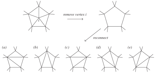
Figure 1: The five possible ways of re-triangulate after removing a node of order five. Choosing one of these possibilities at random yields a blocked triangulation. If a node of order six is removed there are 42 ways of reconnecting.

By iterating this procedure an arbitrary number of times we can produce a blocked triangulation of any volume. In practice, this procedure is effected by randomly flipping the links around the selected node until its coordination number becomes equal to three. At this point any curvature associated with the node has been smeared out over its neighbors. We then remove the three-fold node. It is trivial to see that this method preserves the integrated curvature within a sufficiently large loop around the node in question. However it is not at all obvious that this is enough to capture the most important long distance physics governing the fractal structure, critical exponents etc. We examine these issues now.

4 Pure gravity

We have applied this blocking method to the case of pure gravity (triangulations taken with weight unity) and performed a series of Monte Carlo simulations on lattices ranging from 250 to 4000 nodes. A standard link flip algorithm was used to explore the space of configurations and typically $10^{6}$ sweeps performed for each lattice volume. Every twenty sweeps a configuration was picked out and blocked several times down to 8 nodes.

4.1 The fractal structure

To see whether the long distance physics of the surfaces is being preserved we have measured two exponents which describe complementary features of the fractal structure; the string susceptibility exponent $\gamma_{s}$ and the Hausdorff or fractal dimension $d_{H}$.

The string susceptibility exponent is related to the large volume behavior of the fixed area partition function $Z(N)$,

$$Z(N)\;\sim\;N^{\gamma_{s}-3}\;e^{\mu_{c}N}.$$ (13)

In the case of pure gravity $\gamma_{s}=-1/2$. An efficient method for measuring $\gamma_{s}$ in numerical simulations is to look at the distribution of so-called minbu’s (minimal neck baby universes) [6, 7]. A minbu is a part of a triangulation which is connected to the rest through a neck or a loop consisting of three links. The distribution of minbu’s can be calculated from the number of ways a baby universe of volume $B$ can be glued onto a surface of volume $N-B$;

$$n_{N}(B)\;=\;\frac{B\;Z(B)\>(N-B)\>Z(N-B)}{Z(N)}\;\sim\;(N-B)^{\gamma_{s}-2}\;B^{\gamma_{s}-2}.$$ (14)

It is easy to measure this distribution numerically and the exponent $\gamma_{s}$ is obtained by fitting to Eq. (14). The accuracy of the fit can be improved considerably by including a $1/B$ correction term.

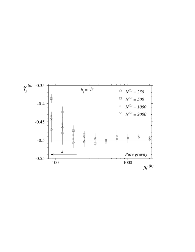
Figure 2: $\gamma_{s}$ for ensembles of surfaces obtained by blocking pure gravity triangulations $k$ times. The values are plotted versus volume and the blocking increases in the left direction.

We have measured $\gamma_{s}$ in this way for the ensemble of triangulations $T^{(k)}$ obtained by blocking $k$ times. The result is shown in Fig. 2 where we plot $\gamma_{s}^{(k)}$ versus volume. This is done for four different initial volumes $N^{(0)}$. It should be noted that the number of blocking steps increases to the left in the plot. It is clear from Fig. 2 that independent of the initial volume and number of blocking steps we get the correct value of $\gamma_{s}$ down to volumes of size 200 nodes. For smaller volumes it is hard to measure $\gamma_{s}$ accurately due to finite size effects. This demonstrates that even after removing 90% of the initial triangulation by blocking the model remains in the universality class of pure gravity.

Additional evidence is obtained by measuring the Hausdorff dimension of the surfaces. It has recently been shown that the Hausdorff dimension is related to point-point distributions on the triangulations and that it can be measured numerically by looking at their scaling behavior [8, 9]. The point-point distributions $n(r,N)$ are defined as the number of nodes at a geodesic distance $r$ from some random origin. Given that the system is close to criticality, it is plausible and indeed appears correct, that these distributions satisfy a scaling ansatz for large $N$. This implies that

$$n(r,N)\;=\;N^{y}\;f\left(r/N^{x}\right)\>=\;N^{1-1/d_{H}}\>f\left({r\over N^{1/d_{H}}}\right).$$ (15)

The scaling exponents $x$ and $y$ are fixed by assuming that there exist a power-law relation between a length scale $l$ and volume N, $N\propto l^{d_{H}}$, and by noting that the integral of $n(r,N)$ yields the total volume.

In numerical simulations $d_{H}$ can be extracted by measuring $n(r,N)$ at different volumes and find the optimal value that collapses all the data onto a single curve using Eq. (15). The scaling assumption also implies that both the position $r_{0}$ and height $n(r_{0})$ of the peak in $n\left(r,N\right)$ should scale simply with volume $N$, i.e.

$$r_{0}\sim N^{1\over d_{H}}\;\;\;\;\;{\rm and}\;\;\;\;\;n(r_{0})\sim N^{1-{1\over d_{H}}}.$$ (16)

In Table 1 we show $d_{H}$ measured using the relations Eq. (16) on volumes ranging from 250 to 1000 nodes. This is shown both for the initial (unblocked) lattices, and for ensembles obtained by blocking once or twice. It is clear that the extracted Hausdorff dimension for the blocked ensembles is completely in agreement with its value extracted from the bare lattice $d_{H}=3.15(2)$. But note that these results are far from the exact result $d_{H}=4$. This effect has been observed before and is attributed to the presence of large corrections to scaling in the current lattice ensemble in which degenerate links are excluded. In [8] it was shown that this estimate moves up to be statistically consistent with four if a wider ensemble is used in which tadpole and self-energy insertions are included.

It is more instructive to compare the distributions directly. In Fig. 3 we plot distributions at volume $N=250$, both for blocked and unblocked triangulations. This is compared to an estimate of the infinite volume distribution $n(r,\infty)$. (the distribution $n(r,\infty)$ is obtained by scaling a distribution corresponding to a large volume ($N=2000$) down to $N=250$ using Eq. (15) with the exact value $d_{H}=4$). The finite size effects are very apparent in Fig. 3 as both distributions deviate from $n(r,\infty)$. But it is intriguing that the curve corresponding to the blocked $N=250$ ensemble is closer to the estimated continuum curve - perhaps the first indication that the blocking is resulting in a flow towards a fixed point.

$k$		$d_{H}(r_{0})$		$d_{H}(n_{max})$
0		3.15(2)		3.13(1)
1		3.16(2)		3.15(1)
2		3.15(2)		3.20(1)

Table 1: The Hausdorff dimension $d_{H}$ extracted both from the scaling of the location of the peak in $n(r,N)$ and its maximal value. Results are shown for different number of blocking steps $k$ with $b_{l}=2$. The volumes used are from 250 to 1000 nodes.

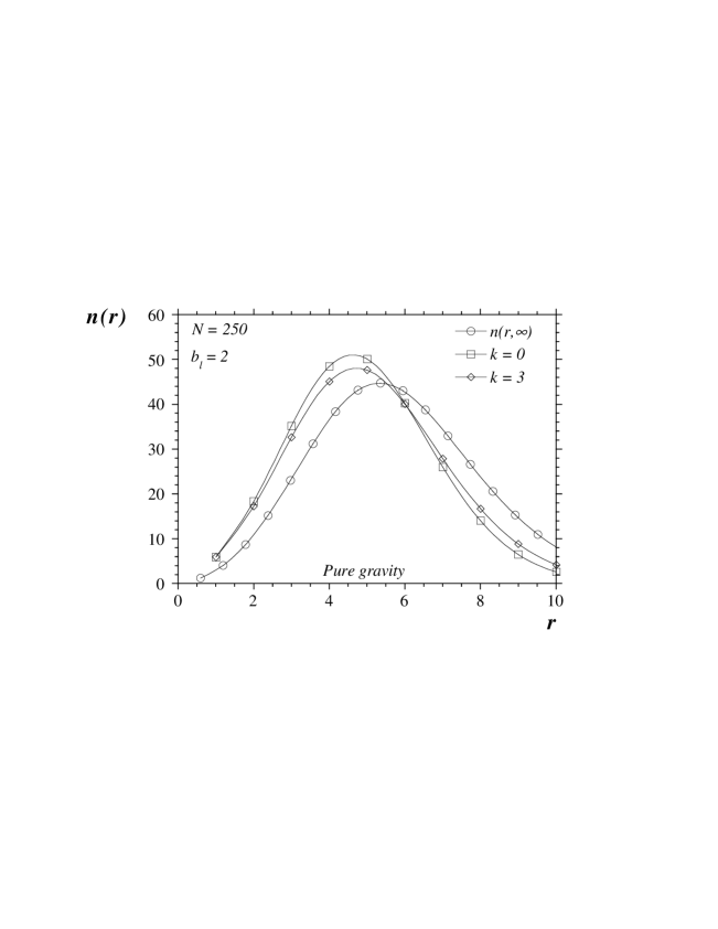
Figure 3: The point-point distributions $n(r,N)$ for $N=250$ in the case of pure gravity. Data for both blocked (87.5%) and unblocked triangulations is compared to an estimate of the continuum distribution $n(r,\infty)$.

Combined the measurements of $\gamma_{s}$ and $d_{H}$ for the ensemble of blocked manifolds provide strong evidence that the fractal structure is preserved. This gives us confidence that the DB method correctly captures the long distance physics of the model.

4.2 Fixed point behavior

It is not enough that the RG transformation preserves the fractal structure, it should also induce a flow in the couplings towards a critical (unstable) fixed point. Optimally we would like to study the behavior of relevant operators around that fixed point and extract some critical exponents. Unfortunately for pure gravity the only simple relevant operator corresponds to the area operator, which is not accessible to us as we are working in the fixed area (volume) ensemble.

Instead we have looked at the behavior of expectation values of various irrelevant operators constructed out of the local coordination number $q_{i}$ or curvature $\left(6-q_{i}\right)$. Specifically we have looked at the following operators (where the superscript $k$ labels the blocking level):

$$\left<O_{1}^{\left(k\right)}\right> = \left<{1\over N^{\left(k\right)}}\sum_{i}\left(q_{i}^{\left(k\right)}-6\right)^{2}\right>,$$ (17)

$$\left<O_{2}^{\left(k\right)}\right> = \left<{1\over N^{\left(k\right)}}\sum_{\left<ij\right>}\left(q_{i}^{\left(k\right)}-6\right)\left(q_{j}^{\left(k\right)}-6\right)\right>.$$ (18)

$\left<ij\right>$ implies that the sum is over neighboring nodes.

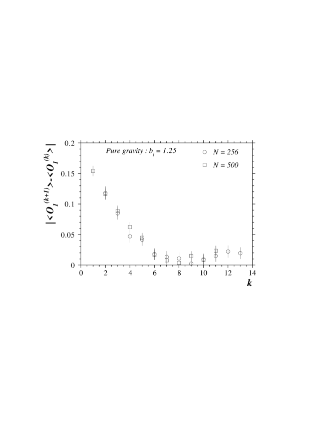
Figure 4: Differences in expectation values of the operator $O_{1}^{(k)}$ for surfaces obtained with different amount of blocking (but with the same volume).

If a fixed point exists then we would expect that in the absence of finite size effects (i.e. the initial lattice is lying on the critical surface) that these operators flow under repeated blocking into the fixed point. Thus differences of the expectation values between blocking levels should vanish;

$$\left|\left<O_{i}^{\left(k+1\right)}\right>-\left<O_{i}^{\left(k\right)}\right>\right|\to 0\;,\qquad k\to\infty.$$ (19)

Since we are forced to work with finite volumes we have to be careful in how we compare these operator expectation values. It only makes sense to compare operator expectation values at the same volume, but differing in the number of blocking steps. This we do in Fig. 4. We have simulated at different initial volumes $N^{(0)}$ (500 to 8000 nodes) which then are blocked down to fixed volume (256 or 500 nodes) using a blocking factor $b_{l}=5/4$. Then the difference Eq. 19 is constructed. Clearly after just a few blocking steps this operator difference is close to zero. Similar results are observed in other channels and give strong evidence of the existence of a fixed point in the model. Combined with the previous demonstrations regarding $\gamma_{s}$ and $d_{H}$ it appears that the decimation method is a rather promising approach to a real-space RG for pure gravity.

4.3 Higher derivative curvature term

How robust is the ND method? To answer that we have studied the RG flow of other operators which are thought to be irrelevant for pure gravity. One such operator is $\;O=\sum_{i}\log{q_{i}}\;$ which corresponds to a set of higher derivative curvature interactions. The non-perturbative flows of this operator have been examined previously in the context of the LGB method [10].

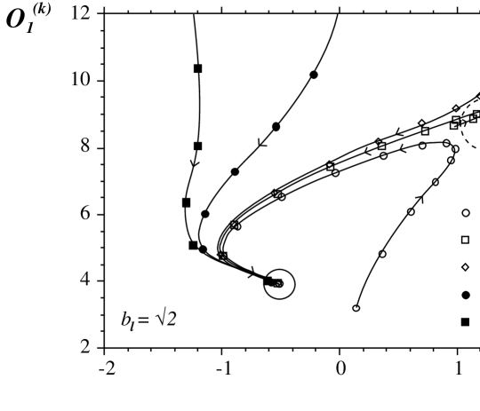
Figure 5: The RG flow of the curvature operators $O_{1}$ and $O_{2}$ as an ensemble of triangulations is blocked. The flow is shown for different values of the bare coupling $\alpha$. The dashed circle indicates an unstable fixed point, the solid a zero volume sink.

The idea is to add such a term to the bare action with some coupling $\alpha$. Under blocking the coupling to this new term should be driven to zero in the effective action as it corresponds to an irrelevant operator. Thus expectation values of operators should approach their values in the model without this extra interaction term. This is illustrated in Fig. 5 were we plot the RG trajectory in the ($O_{1}$,$O_{2}$) plane for a range of bare couplings $\alpha$.

We see that while the flows for different bare $\alpha$ start out from different points in the plane, for sufficiently positive $\alpha$ they are all attracted towards a fixed point. After passing close to this point the flows converge on a unique ‘renormalized’ trajectory which ends at a trivial fixed point corresponding to zero volume triangulations.

However, there are some indications that this no longer is true for sufficiently large negative values of $\alpha$ (the solid points). There the expectation values start to deviate considerable from the pure gravity values. At these lattice volumes they never pass close to the unstable fixed point but run smoothly to the trivial end point. Such an effect has been observed before and it is believed that for large negative $\alpha$ the model enters a ‘super-crumpled’ state [11].

$k$	$N^{(k)}$	$\alpha=10$	$\alpha=5$	$\alpha=1$	$\alpha=-1$	$\alpha=-5$	$\alpha=-10$
0	1000	-0.47(1)	-0.47(2)	-0.48(1)	-0.49(1)	-0.03(3)	2.1(1)
1	500	-0.49(1)	-0.47(2)	-0.50(1)	-0.48(1)	-0.30(2)	1.8(2)
2	250	-0.51(2)	-0.46(2)	-0.47(2)	-0.48(2)	-0.53(2)	2.0(2)
3	125	-0.47(1)	-0.42(2)	-0.46(2)	-0.42(1)	-0.65(3)	0.5(2)

Table 2: $\gamma_{s}^{(k)}$ for ensembles of triangulations obtained by blocking $k$ times. Results are shown for various values of the bare coupling $\alpha$.

Such an effect is also observed in the fractal structure. We have measured the string susceptibility exponent as before for several values of $\alpha$ and various number of blocking steps. The result is shown in Table 2. For $10\geq\alpha\geq-1$ we get consistently the pure gravity value. But for $\alpha=-5$ the initial ensemble yields a different value of $\gamma_{s}$; but as it is blocked the value appears to flow towards the pure gravity fixed point value. For $\alpha=-10$ the fractal structure is dramatically changed, we get a consistent value of $\gamma_{s}\approx 2$, even after considerable blocking.

It is not clear at present whether these results can be explained on the basis of finite size effects which are much more dramatic for large negative $\alpha$ or whether they indicate that no continuum limit exists for such models - the trajectories are never attracted towards the usual unstable fixed point. Certainly we have not observed any non-trivial new fixed points associated with these negative coupling flows.

5 Ising model coupled to 2d gravity

The next step is to apply the method to matter fields living on the surfaces. For that purpose we chose Ising spins coupled to gravity in which case the matter contribution to the partition function Eq. (10) is

$$Z_{M}(T)\;=\;\sum_{\{\sigma_{i}\}}{\rm e}^{\textstyle\;\beta\sum_{\left<ij\right>}\sigma_{i}\sigma_{j}}.$$ (20)

Here the sum runs over each edge length in a triangulation and the coupling $\beta$ is tuned to its critical value.

This model is exactly solvable [13] so we know the critical coupling, $\beta_{c}=\frac{1}{2}\log{\frac{131}{85}}$, together with the exponents governing the critical behavior. In addition we know the effect the matter has on the fractal structure. The Ising spins only change the string susceptibility exponent at the critical point to $\gamma_{s}=-1/3$, elsewhere it retains the pure gravity value.

We have simulated this model at the critical point of the Ising model for lattice volumes $N=500,1000$ and 2000 nodes. A Swendsen-Wang cluster algorithm was used to update the spins and again about $10^{6}$ sweeps performed per lattice volume.

5.1 Blocking the spin configurations

When it comes to extending the ND method to block a spin configuration, in addition to a triangulation, we have to decide to what extent the blocking of the gravitational sector and spin sector should influence each other. The simplest solution is that the blocking of the triangulations should be performed precisely as for pure gravity - the only effect of the critical matter will be to alter the initial distribution of triangulations. When a given blocking ratio has been obtained a new spin configuration is created from the spin configuration of the initial triangulation.

To block the spin configuration we choose the ”majority-rule” transformation that has been applied successfully to the Ising model on a regular lattice. The spins on neighboring nodes are grouped into ”blocks” and a block spin value assigned to each block depending on the sum of its spins. If the sum is positive the value is +1 but -1 if it is negative. If the sum is zero we assign +1 and -1 with equal probability. However, there is a difference in applying this method to random surfaces as opposed to a regular lattice. A regular lattice can be divided into equal non-intersecting blocks, an arbitrary triangulation not. Instead we define a ”block” as a spin that survives the decimation together with the neighbors it had before blocking. This definition is appealing as it incorporates the influences of the geometry. The size of the ”spin-blocks” will be depend on the local curvature.

However, there is still an ambiguity in this definition of ”spin-blocks”. Some spins will contribute to more than one such block, in particular if two neighboring nodes both survive the decimation. This is especially true if a small blocking ratio is used. Thus it might be necessary to limit the influence of such nodes by excluding them from other blocks than their own. We tried this modified definition of spin-blocks, but it did not change the results appreciably.

5.2 The fractal structure

How well does the node decimation preserve the fractal structure for this model? Again we have computed the string susceptibility exponent; the result is shown in Fig. 6 for three different initial volumes. Notice that as the blocking of the geometry is independent of the spins the results do not depend on the definition of spin-blocks.

Figure 6: Changes in $\gamma_{s}$ as triangulations with Ising spins are blocked. Data is shown for three initial volumes. Again the number of blocking steps $k$ increases to the left. The horizontal line is the exact value $\gamma_{s}=-1/3$.

The first thing to notice is that without any blocking we measure the value $\gamma_{s}\approx-0.41$, which is somewhat lower than the theoretical value $\gamma_{s}=-1/3$. This is due to the fact that we measure at the infinite volume critical coupling $\beta_{c}^{\infty}$ not the pseudo-critical coupling $\beta_{c}^{V}$ appropriate for the finite volume used. This effect has been observed in earlier numerical estimates of $\gamma_{s}$ for this model in [7]. There a sharp peak was observed around $\beta_{c}^{V}$ with peak value $\gamma_{s}\approx-1/3$. But away from the peak the values rapidly return to the pure gravity value $\gamma_{s}=-1/2$. As the volume is increased the peak moves closer to the true critical point.

However under blocking the measured $\gamma_{s}$ appears to flow towards the exact value. This, of course, is very encouraging from the point of view of capturing fixed point physics. Notice that direct simulations of the smallest volume lattices would have produced estimates for $\gamma_{s}$ further from the exact result.

5.3 Scaling exponents

To measure the critical exponents of the Ising model we consider several operators constructed out of products of neighboring spins and apply the methods described in section 2. In practice the possible operators can be classified according to their symmetry properties under the $Z(2)$ operation $\sigma_{i}\to-\sigma_{i}$. In the linearized matrix $T_{\alpha\beta}$ the cross-correlations between these even and odd operators vanish.

In the odd sector we have looked at the operators

$$S^{o}_{1}\;=\;\sum_{i}\sigma_{i}\;\;\;\;\;{\rm and}\;\;\;\;\;S^{o}_{2}\;=\;\sum_{\left<ijk\right>}\sigma_{i}\sigma_{j}\sigma_{k},$$ (21)

where the first sum is over nodes and the second over triangles $\left<ijk\right>$. For the even sector we have chosen the operators

$$S^{e}_{1}\;=\;\sum_{\left<ij\right>}\sigma_{i}\sigma_{j}\;,\;\;\;\;\;S^{e}_{2}\;=\;\sum_{\left<kl\right>^{\prime}}\sigma_{k}\sigma_{l}\;\;\;\;\;{\rm and}\;\;\;\;\;S^{e}_{3}\;=\;\sum_{\left<ijkl\right>}\sigma_{i}\sigma_{j}\sigma_{k}\sigma_{l}.$$ (22)

The indices $i,j,k,l$ refer to an elementary link $ij$ together with the complementary vertices $k,l$ associated with the two neighboring triangles.

These operators allow us to determine numerically two scaling exponents; the magnetic exponent $y_{1}$ and the thermal exponent $y_{2}$. The former corresponds to the odd operators, the latter to the even. These scaling exponents are related to the critical exponents of the Ising model $\nu$ and $\delta$ through the relations

$$y_{1}\;=\;\frac{\delta}{\delta+1}\;\;\;\;\;\;{\rm and}\;\;\;\;\;\;y_{2}\;=\;\frac{1}{\nu d_{H}}.$$ (23)

For the Ising model coupled to gravity these critical exponents are known, $\nu d_{H}=3$ and $\delta=5$, yielding the values $y_{1}=5/6$ and $y_{2}=1/3$ for the scaling exponents. In comparison, for the Ising model on a flat regular lattice these exponents are $y_{1}=15/16$ and $y_{2}=1/2$.

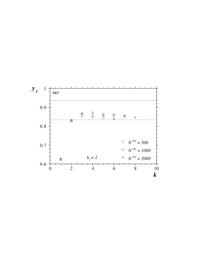
Figure 7: The scaling exponents $y_{1}$ and $y_{2}$, corresponding to odd and even spin operators respectively, versus the number of RG iterations $k$. In both plots the lower horizontal lines are the exact values for an Ising model coupled to gravity $y_{1}=5/6$ and $y_{2}=1/3$, while the upper lines are the flat space values $y_{1}=15/16$ and $y_{2}=1/2$.

In Figs. 7$a$ and $b$ we show the extracted values of the scaling exponents as a function of the RG iterations $k$ using a blocking ratio $b_{l}=2$ (and for different initial volumes). The values shown are obtained including only one spin operator for each sector in the calculation of the matrix $T_{\alpha\beta}$, i.e. $S^{o}_{1}$ and $S^{e}_{1}$. With the accuracy we have at present no obvious improvement was observed by enlarging the operator basis (although the results were perfectly compatible).

The results show that after one or two blocking steps we have approached a critical fixed point. It clearly is the correct one as we get results which agree with the exact values within 2 or 3% accuracy. In comparison the exponents for the Ising model on a flat lattice are clearly ruled out. It is impressive that even after blocking down to triangulations consisting only of 16 nodes the critical exponents of the Ising model still come out correctly.

Do these results depend on the blocking ratio? Unlike for the triangulations the blocking of the spin configurations is not independent of the amount of node decimation. We tried three different blocking ratios, $b_{l}=\sqrt{2}$, 2 and 4, but the results did not change very much. The error-bars increased somewhat as the blocking ratio was decreased, which is not unexpected.

6 Alternative blocking methods

As mentioned in the introduction there are other real-space RG transformations that have been proposed for random surfaces. But how well do those methods capture the long distance physics of the surfaces? We have investigated this for the local geodesic blocking (LGB) method.

A brief description of the method given in [3]: Given a triangulation $T(N)$ we chose a subset of $N^{\prime}$ nodes and connect them together to form a block triangulation $T^{\prime}$. This is done in such way as to preserve locally the relative geodesic distances between block nodes. In practice the subset of nodes is fixed at the beginning of the simulations. The initial triangulation is then evolved using a standard link flip algorithm and simultaneously the block triangulation is updated with the prescription that a link $l_{ij}$ is flipped to $l_{kl}$ if the geodesic distance $d_{kl}$ is less than $d_{ij}$ (measured on the unblocked lattice). That this constraint is local is essential for the algorithm to be practical in numerical simulations.

We have measured the distribution of baby universes on the ensemble of triangulations created by this blocking method, both for surfaces with spherical and toroidal topology (the latter was used in [3]). The result for $\gamma_{s}$ are shown in Table 3. They indicate that the fractal structure is not correctly preserved. The ensemble of blocked triangulations has, consistently, $\gamma_{s}\approx 0.28$ independent of blocking ratio or topology.

		$k=0$		$k=1$		$k=2$
	$b_{l}$	$N$	$\gamma_{s}$	$N$	$\gamma_{s}$	$N$	$\gamma_{s}$
Sphere
	1.08	270	-0.504(14)	250	0.271(18)
	1.2	300	-0.506(13)	250	0.280(11)
	1.6	400	-0.486(16)	250	0.296(27)
	2.0	500	-0.484(17)	250	0.273(30)
	4.0	1000	-0.499(11)	250	0.289(40)
Torus
	4	2304	-0.486(16)	576	0.306(27)	144	0.281(30)
	4	1024	-0.504(9)	256	0.268(35)

Table 3: Measured values of $\gamma_{s}$ for triangulations blocked with the LGB method. Results are shown for both spherical and toroidal topologies and for various blocking ratios $b_{l}$.

This is in our opinion a serious flaw of the method. If $\gamma_{s}$ is thought of as a regular critical exponent this result would imply that this RG scheme is driving the system towards a new fixed point - not pure two-dimensional gravity. A possible explanation is that as the method uses local constraints to dictate the link flips on the block triangulations, it may actually simulate the effect of having some kind of matter field living on the manifolds. This could effectively change the physics of the model.

The situation might be improved by using a generalization of the LGB method; a global geodesic blocking (GGB). It is defined by requiring that the block triangulation preserves (up to an overall global length rescaling) as closely as possible all possible geodesic paths between block nodes. In practice this may be implemented by minimizing a cost function $E$ when performing block lattice link flips

$$E=\sum_{ij}\left(d_{ij}-\lambda d^{\prime}_{ij}\right)^{2}.$$ (24)

The quantities $d_{ij}$ and $d_{ij}^{\prime}$ are the distances in units of the cut-off between block nodes $i$ and $j$ defined on both the initial lattice and block lattice respectively. The parameter $\lambda$ relates the two scales and may be chosen so as to minimize $E$ for fixed lattices. Clearly other choices of $E$ are possible corresponding, for example, to weighting small and long geodesics differently.

We have investigated this method numerically, using the cost function Eq. (24) and found that it indeed seems to cure the problem of an incorrect $\gamma_{s}$ exponent. The values of $\gamma_{s}$, obtained with limited statistics, are consistent with the pure gravity value. Unfortunately as the method is highly nonlocal it is computationally burdensome and not feasible in practice.

7 Outlook

We have presented results on a new real-space renormalization group method for dynamically triangulated $2d$ gravity. Our results are encouraging in so far as they indicate that under a simple node decimation (ND) flows toward a fixed point in the critical surface are produced. Measurements of the string susceptibility and Hausdorff dimension strongly support the notion that this fixed point corresponds to $2d$ quantum gravity. The effect of including an irrelevant operator corresponding to a higher order curvature term also support this picture. Indeed the demonstrated irrelevance of such an operator outside of perturbation theory might be taken as the first successful non-trivial application of the method.

We have extended the method to a simple critical Ising system coupled to $2d$ gravity and have been able to extract exponents in excellent agreement with the predictions for gravitational dressing given by the DDK/KPZ formula [14]. Furthermore measurements of the string susceptibility exponents indicate that the finite size effects are significantly reduced. This provides further evidence for a flow to the correct fixed point.

There is still some scope for improving the method. A more systematic investigation of how to inter-disperse the node and spin blocking would be desirable. Also the effects of employing a more extensive operator basis should be studied.

Provided the method or refinements thereof survive these tests the way is open to apply these RG methods to a variety of unsolved problems in $2d$ gravity.

Acknowledgements

We would like to acknowledge stimulating conversations during the course of this work with Mark Bowick, Varghese John, John Kogut and Ray Renken. This work was supported by research funds provided by Syracuse University and the computational facilities of NPAC.

References

-
[1]
F. David, ”Simplicial Quantum Gravity and Random Lattices“,
(hep-th/9303127), Lectures given at Les Houches Summer School
on Gravitation and Quantization, Session LVII,
Les Houches, France, 1992;
J. Ambjørn, ”Quantization of Geometry“, (hep-th/9411179), Lectures given at Les Houches Summer School on Fluctuating Geometries and Statistical Mechanics, Session LXII, Les Houches, France 1994;
P. Di Francesco, P. Ginzparg and J. Zinn-Justin, Phys. Rep. 254 (1995) 1. -
[2]
J. Ambjørn, B. Durhuus, T. Jonsson and G. Thorleifsson,
Nucl. Phys. B398 (1993) 568;
J. Ambjørn, G. Thorleifsson and M. Wexler, Nucl. Phys. B439 (1995) 187;
C. Baillie and D. Johnston, Phys. Lett. B286 (1992) 44; Mod. Phys. Lett. A7 (1992) 1519;
M. Bowick, M. Falcioni, G. Harris and E. Marinari, Nucl. Phys. B419 (1994) 665;
S. Catterall, J. Kogut and R. Renken, Nucl. Phys. B292 (1992) 277; Phys. Rev. D45 (1992) 2957;
J. Jurkiewicz, A. Krzywicki, B. Petersson and B. Soderberg, Phys. Lett. B213 (1988) 511. - [3] R. Renken, Phys. Rev. D50 (1994) 5130.
-
[4]
D. Johnston, J.P.Kownacki and A. Krzywicki, ”Random
Geometries and Real Space Renormalization Group“,
(hep-lat/9407018), LPTHE-Orsay-94-70;
Z. Burda, J.P. Kownacki and A. Krzywicki, Phys. Lett. B356 (1995) 466. - [5] R.H. Swendsen in ”Real-Space Renormalization, Topics in Current Physics“ Vol. 30, eds. T.W. Burkhardt and J.M.J. van Leeuwen (Springer, Berlin, 1982) pg. 57.
- [6] S. Jain and S.D. Mathur, Phys. Lett. B286 (1992) 239.
-
[7]
J. Ambjørn, S. Jain and G. Thorleifsson, Phys. Lett.
B397 (1993) 34;
J. Ambjørn and G. Thorleifsson, Phys. Lett. B323 (1994) 7. - [8] S. Catterall, G. Thorleifsson, M. Bowick and V. John, Phys. Lett. B354 (1995) 58.
- [9] J. Ambjørn, J. Jurkiewicz and Y. Watabiki, ”On the Fractal Structure of Two-Dimensional Quantum Gravity“, (hep-lat/9507014), NBI-HE-95-22.
- [10] R. Renken, S. Catterall and J. Kogut, Phys. Lett. B345 (1995) 422.
- [11] D. Boulatov, V. Kazakov, I.K. Kostov and A.A. Migdal, Nucl. Phys. B275 (1986) 641.
- [12] J. Ambjørn, S. Jain, J. Jurkiewicz and C.F. Kristjansen, Phys. Lett. B305 (1993) 208.
-
[13]
V.A. Kazakov, Phys. Lett. A119 (1986) 140;
D. Boulatov and V.A. Kazakov, Phys. Lett. B186 (1987) 379. -
[14]
F. David, Mod. Phys. Lett. A3 (1988) 1651;
J. Distler and H. Kawai, Nucl. Phys. B321 (1989) 509;
V.G. Knizhnik, A.M. Polyakov and A. Zamolodchikov, Mod. Phys. Lett. A3 (1988) 819.