Abstract

We present the lattice gauge theory approach to evaluating non-perturbative hadronic interactions from first principles. We discuss applications to glueballs, inter-quark potentials, the running coupling constant, the light hadron spectrum and the pseudoscalar decay constant $f_{P}$.

1 Introduction

The theory of the strong interactions is accurately provided by Quantum Chromodynamics (QCD). The theory is defined in terms of elementary components: quarks and gluons. The only free parameters are the quark mass values (apart from an overall energy scale imposed by the need to regulate the theory). This formulation is essentially the unique candidate for the theory of the strong interactions. The only feasible way to describe a departure from QCD would be in terms of quark and gluon substructure. At least at the energy scales up to which it is tested, there is no evidence for such substructure.

QCD provides a big challenge to theoretical physicists. It is defined in terms of quarks and gluons but the physical particles are composites: the mesons and baryons. Any complete description must then yield these bound states: this requires a non-perturbative approach. One can see the limitations of a perturbative approach by considering the vacuum: this will be approximated in perturbation theory as basically empty with rare quark or gluon loop fluctuations. Such a description will allow quarks and gluons to propagate essentially freely which is not the case experimentally. The true (non-perturbative) vacuum can be better thought of as a disordered medium with whirlpools of colour on different scales. Such a non-perturbative treatment then has the possibility to explain why quarks and gluons do not propagate (ie quark confinement).

The main contender for a non-perturbative description of QCD is the lattice gauge theory approach. Following the ideas of Wilson, space-time is replaced by a discrete grid (the lattice) but gauge invariance is retained exactly. Using also periodic boundary conditions in space and time, the system will have a finite number of degrees of freedom: the gluon and quark fields at the lattice sites. Actually gauge invariance implies that the gluon field lies on the links of the lattice (they correspond to the mechanism that allows colour orientation at different sites to be compared). This finite number of degrees of freedom implies that the theory is a quantum many-body problem rather than a field theory.

The step which makes this many-body problem tractable is to consider Euclidean time. This is perhaps the step which is the most difficult to assess. Formally the quantities to be evaluated can be expressed as Green functions: vacuum expectation values of products of fields. The existence and properties of these Green functions under a Wick rotation to Euclidean time are widely used in perturbative treatments. A non-perturbative determination of the Green functions in the Euclidean time case will lead directly to quantities of relevance in the physical Minkowski time case (eg masses and matrix elements).

With the Euclidean time approach, the formulation of QCD (consider, for example, the functional integral over the gauge fields) is converted into a multiple integral which is well defined mathematically. For a lattice of $L^{4}$ sites with a colour gauge group of SU(3), this would be a $8\times 4\times L^{4}$ dimensional integral (8 from the colour group manifold, $4L^{4}$ from the gauge fields on each link). For any reasonable value of $L$, this is a very high dimension indeed. Simpson’s rule is not the way forward! The standard approach is to use a Monte Carlo approximation to the integrand. This is implemented in an “importance sampling” version so that a stochastic estimate of the integral is made from a finite number of samples (called configurations) of equal weight. The construction of efficient algorithms to achieve this is a topic in itself. Here I will concentrate on the analysis of the outcome, assuming that such configurations have been generated.

So what we have at our disposal is a set of samples of the vacuum. It is then straightforward to evaluate the average of various products of fields over these samples - this gives the Green functions by definition. The Green function can then be continued from Euclidean to Minkowski time (in most cases this is trivial) and compared to experiment.

The validation of the lattice approach calls for a series of checks that everything is under control.

• the lattice spacing should be small enough (discretisation errors)

• the lattice must be big enough in space and time (finite size errors)

• the statistical errors must be under control

• Green functions must be extracted with no contamination (eg a ground state mass could be contaminated with a piece coming from an excited state)

• both the quark contribution to the vacuum (sea quarks) and the quark constituents of hadrons (valence quarks) are usually treated by using larger mass values than the experimental ones and then extrapolating. This extrapolation must be treated accurately.

• a particularly severe approximation is to treat the sea-quarks as of infinite mass. This corresponds to neglecting quark loops in the vacuum and is computationally very much faster. This is known as the “quenched approximation”.

The most subtle of these is the discretisation error. In order to extract the continuum limit of the lattice, one must show that the physical results will not change if the lattice spacing is decreased further. This is subtle because the lattice spacing is not known directly - in effect, it is measured. The lattice simulation is undertaken at a value of a parameter conventionally called $\beta$. In the limit of small coupling $g^{2}$, where perturbation theory applies, $\beta=6/g^{2}$. Thus large $\beta$ corresponds to small $g^{2}$. Now, perturbatively, the coupling $g^{2}$ corresponds to the lattice spacing $a$ as

$$g^{2}\approx{1.0\over b_{0}\log a^{-2}}\ \ \hbox{where}\ \ b_{0}={11-{2\over 3}N_{f}\over 16\pi^{2}}$$

for $N_{f}$ flavours of quarks. For the case of interest, $N_{f}\leq 3$, this corresponds to small values of $g^{2}$ at small distance scale $a$ - as expected from asymptotic freedom.

The perturbative argument is appropriate to the study of results at large $\beta$ (small $g^{2}$). We will find that lattice simulation of QCD uses values of $\beta\approx 6$ and hence bare couplings corresponding to $\alpha=g^{2}/(4\pi)\approx 0.08$. In the pioneering years of lattice work, this was thought to be a sufficiently small number that the perturbation series would converge rapidly. One of the major advances, in recent years, has been the realisation that the bare lattice coupling (our $g^{2}$ above) is a very poor expansion parameter and the perturbation series in the bare coupling does not converge well at the $\beta$ values of interest. The theoretical explanation for this poor convergence is that the lattice Lagrangian differs from the continuum Lagrangian and allows extra interactions. These include tadpole diagrams [11] which have the property that they sum up to give a contribution that involves high order terms in the perturbation series. The way to avoid this problem with tadpole terms is to use a perturbation series in terms of a renormalised coupling - rather than the bare lattice coupling. I return to this topic when discussing the lattice determination of $\alpha_{S}$ later.

This change of attitude to the method of determining $a$ from $\beta$ has had considerable implications for lattice predictions, as I now explain, since we wish to work in a region of lattice spacing $a$ where perturbation theory in the bare coupling is not precise. Because of this, in practice, $a$ is determined from the non-perturbative lattice results themselves. Thus if the energy of some particle is measured on the lattice, it will be available as the dimensionless combination $\hat{E}$. From a value for $E$ in physical units, then $a$ can be determined since, on dimensional grounds, $\hat{E}=Ea$. Furthermore, by increasing $\beta$, the change in the observable $\hat{E}$ gives information about the change in $a$ since $E$ is fixed - assuming it is the physical mass. This should allow a calibration of $\beta$ in terms of $a$ to be established.

This procedure is overly optimistic, however. The discretised lattice theory is different from the continuum theory on scales of the order of the lattice spacing $a$. For the Wilson action formulation of gauge theory, this implies that the continuum energy $E_{c}$ is related to the lattice observable $\hat{E}(\beta)=Ea$ as

$${\hat{E}(\beta)\over a}=E_{c}+{\cal O}(a^{2})$$

A direct consequence is that the ratio of two energies (of different particles, for example) will have discretisation errors of order $a^{2}$.

Thus, to cope with discretisation errors, the procedure required is to evaluate dimensionless ratios of quantities of physical interest at a range of values of the lattice spacing $a$ and then extrapolate the ratio to the continuum limit ($a\to 0$).

Note that when the fermionic terms are included, the discretisation error is of order $a$ for the Wilson fermionic action. By adding further terms in the fermionic action, the error can be reduced - to order $\alpha a$ for the SW-clover fermion formulation.

2 Glueball Masses

I choose to illustrate the workings of the lattice method by describing the determination of the glueball spectrum. Of course, glueballs are only defined unambiguously in the quenched approximation - where quark loops in the vacuum are ignored. In this approximation, glueballs are stable and do not mix with quark - antiquark mesons. This approximation is very easy to implement in lattice studies: the full gluonic action is used but no quark terms are included. This corresponds to a full non-perturbative treatment of the gluonic degrees of freedom in the vacuum. Such a treatment goes much further than models such as the bag model.

The glueball mass can be measured on a lattice through evaluating the correlation $C(t)$ of two closed colour loops (called Wilson loops) at separation $t$ lattice spacings. Formally

$$C(t)=<0|G(0)G^{{\dagger}}(t)|0>=\sum_{i=0}c_{i}<g_{i}(0)|g_{i}(t)>c^{*}_{i}=\sum_{i=0}|c_{i}|^{2}e^{-\hat{m}_{i}t}$$

where $G$ represents the closed colour loop which can be thought of as creating a glueball state $g_{i}$ from the vacuum. Summing over a complete set of such glueball states (strictly these are eigenstates of the lattice transfer matrix where $\exp{-\hat{m}_{i}}$ is the lattice eigenvalue corresponding to a step of one lattice spacing in time) then yields the above expression. As $t\to\infty$, the lightest glueball mass will dominate. This can be expressed as

$$\hat{m}_{0}=\lim_{t\to\infty}\hat{m}_{\rm eff}(t)\ \ \hbox{where}\ \ \hat{m}_{\rm eff}(t)=\log({C(t-1)\over C(t)})$$

Note that since for the excited states $\hat{m}_{i}>\hat{m}_{0}$, then $\hat{m}_{\rm eff}(t)>\hat{m}_{\rm eff}(t+1)>\hat{m}_{0}$. This implies that the effective mass, defined above, is an upper bound on the ground state mass. In practice, sophisticated methods are used to choose loops $G$ such that the correlation $C(t)$ is dominated by the ground state glueball (ie to ensure $|c_{0}|>>|c_{i}|$ ). By using a several different loops, a variational method can be used to achieve this effectively. These techniques are needed to obtain accurate estimates of $\hat{m}_{0}$ from modest values of $t$ since the signal to noise decreases as $t$ is increased. Even so, it is worth keeping in mind that upper limits on the ground state mass are obtained in principle.

The method also needs to be tuned to take account of the many glueballs: with different $J^{PC}$ and different momenta. On the lattice the Lorentz symmetry is reduced to that of a hypercube. Non-zero momentum sates can be created (momentum is discrete in units of $2\pi/L$ where $L$ is the lattice spatial size). The usual relationship between energy and momentum is found for sufficiently small lattice spacing. Here we shall concentrate on the simplest case of zero momentum (obtained by summing the correlations over the whole spatial volume).

For a state at rest, the rotational symmetry becomes a cubic symmetry. The lattice states (the $g_{i}$ above) will transform under irreducible representations of this cubic symmetry group (called $O_{h}$). These irreducible representations can be linked to the representations of the full rotation group SU(2). Thus, for example, the five spin components of a $J^{PC}=2^{++}$ state should be appear as the two-dimensional E⁺⁺ and the three-dimensional T${}_{2}^{++}$ representations on the lattice, with degenerate masses. This degeneracy requirement then provides a test for the restoration of rotational invariance - which is expected to occur at sufficiently small lattice spacing.

The results of lattice measurements [1, 2, 3, 4] of the $0^{++}$ and $2^{++}$ states are shown in fig 1. The restoration of rotational invariance is shown by the degeneracy of the two $O_{h}$ representations that make up the $2^{++}$ state. Fig 1 shows the dimensionless combination of the lattice glueball mass $\hat{m}_{0}$ to a lattice quantity $\hat{r}_{0}$. We will return to describe the lattice determination of $\hat{r}_{0}$ in more detail - here it suffices to accept it as a well measured quantity on the lattice that can be used to calibrate the lattice spacing and so explore the continuum limit. The quantity plotted, $\hat{m}_{0}\hat{r}_{0}$, is expected to be equal to the product of continuum quantities $m_{0}r_{0}$ up to corrections of order $a^{2}$. This is indeed seen to be the case. The extrapolation to the continuum limit ($a\to 0$) can then be made with confidence.

The value of $r_{0}$ in physical units is about 0.5 fm and we will adopt a scale equivalent to $r_{0}^{-1}=0.372$ GeV. This information yields lattice predictions for the glueball masses of around 1.6 GeV and 2.2 GeV for the $0^{++}$ and $2^{++}$ glueballs respectively.

We return briefly to the independence of the results on the volume of the lattice. In the early days of glueball mass determination, it was expected that a spatial size $L$ should satisfy $\hat{m}(0^{++})L>1$ and, hence, that values of $\hat{m}(0^{++})L$ of 1 to 4 would suffice. A careful lattice study [12] showed that $\hat{m}(0^{++})L>8$ was required to obtain rotational invariance and a result independent of $L$. The results collected in fig 1 all satisfy this latter inequality so can be regarded as the infinite volume determination.

Figure 1: The value of mass of the $J^{PC}=0^{++}$ and $2^{++}$ glueball states from refs[1, 2, 3, 4] in units of $r_{0}$. The $T_{2}$ and $E$ representations are shown by octagons and diamonds respectively. The straight line shows a fit describing the approach to the continuum limit as $a\to 0$.

The predictions for the other $J^{PC}$ states are that they lie higher in mass and the present state of knowledge is summarised in fig 2. Remember that the lattice results are strictly upper limits. For the $J^{PC}$ values not shown, these upper limits are too weak to be of use.

Since quark - antiquark mesons can only have certain $J^{PC}$ values, it is of special interest to look for glueball with $J^{PC}$ values not allowed for such mesons: $0^{--},0^{+-},1^{-+},2^{+-},$ etc. Such spin-exotic states, often called “oddballs”, would not mix directly with quark - antiquark mesons. This would make them a very clear experimental signal of the underlying glue dynamics. Various glueball models (bag models, flux tube models, QCD sum-rule inspired models,..) gave different predictions for the presence of such oddballs (eg. $1^{-+}$) at relatively low masses. The lattice mass spectra clarify these uncertainties but, unfortunately for experimentalists, do not indicate any low-lying oddball candidates. The lightest candidate is from the T${}_{2}^{+-}$ spin combination. Such a state could correspond to an $2^{+-}$ oddball. Another interpretation is also possible, however, namely that a non-exotic $3^{+-}$ state is responsible (this choice of interpretation can be resolved in principle by finding the degenerate 5 or 7 states of a $J=2$ or 3 meson). The overall conclusion at present is that there is no evidence for any oddballs of mass less than 3 GeV.

Glueballs are defined in the quenched approximation and, hence, they do not decay into mesons since that would require quark - antiquark creation. It is, nevertheless, still possible to estimate the strength of the matrix element between a glueball and a pair of mesons within the quenched approximation. For the glueball to be a relatively narrow state, this matrix element must be small. A very preliminary attempt has been made to estimate the size of the coupling of the $0^{++}$ glueball to two pseudoscalar mesons [5]. A relatively small value is found. Further work needs to be done to investigate this in more detail, in particular to study the mixing between the glueball and $0^{++}$ mesons since this mixing may be an important factor in the decay process.

Another lattice study will become feasible soon. This is to study the glueball spectrum in full QCD vacua with sea quarks of mass $m_{D}$. For large $m_{D}$, the result is just the quenched result described above. For $m_{D}$ equal to the experimental light quark masses, the results should just reproduce the experimental meson spectrum - with the resultant uncertainty between glueball interpretations and other interpretations. The lattice enables these uncertainties to be resolved in principle: one obtains the spectrum for a range of values of $m_{D}$ between these limiting cases, so mapping glueball states at large $m_{D}$ to the experimental spectrum at light $m_{D}$.

Figure 2: The mass of the glueball states with quantum numbers $J^{PC}$ from ref[3]. The scale is set by ${\sqrt{\sigma}}\approx 0.44$ GeV which yields the right hand scale in GeV. The solid points represent mass determinations whereas the open points are upper limits.

3 Potentials between quarks

A very straightforward quantity to determine from lattice simulation is the interquark potential in the limit of very heavy quarks (static limit). This potential is of direct physical interest because solving the Schrödinger equation in such a potential provides a good approximation to the $\Upsilon$ spectrum. It is also relevant to exploring both confinement and asymptotic freedom on a lattice.

The basic route to the static potential is to evaluate the average $W(\hat{R},\hat{T})$ in the vacuum samples of a rectangular closed loop of colour flux (a Wilson loop of size $\hat{R}\times\hat{T}$). here the lattice quantities $\hat{R}$ and $\hat{T}$ are related to the physical distances $R$ and $T$ by $\hat{R}=R/a$, etc where $a$ is the lattice spacing which is not known explicitly. Then it can be shown that the required static potential in lattice units is given by

$$\hat{V}(\hat{R})=\lim_{\hat{T}\to\infty}\log{W(\hat{R},\hat{T}-1)\over W(\hat{R},\hat{T})}$$

The limit of large $T$ is need to separate the required potential from excited potentials. This limit can be made tractable in practice by using more complicated loops than the simple rectangular loop described above.

A summary of results [6] for the potential at large $R$ is shown in fig 3. The result that the force $dV/dR$ tends to a constant at large $R$ (and thus $V(R)$ continues to rise as $R$ increases) is a manifestation of the confinement of heavy quarks (in the quenched approximation). The force appears to approach a constant at large $R$. A simple parametrisation is traditional in this field:

$$V(R)=V_{0}-{e\over R}+KR$$

where $K$ (sometimes written $\sigma$) is the string tension. The term $e/R$ is referred to as the Coulombic part in analogy to the electromagnetic case. The equivalent relationship in terms of quantities defined on a lattice is

$$\hat{V}(\hat{R})=\hat{V}_{0}-{e\over\hat{R}}+\hat{K}\hat{R}$$

where the lattice string tension $\hat{K}=Ka^{2}$.

Figure 3: The force between static quarks at separation $r$ as measured on lattice with different lattice spacing $a$ (with the $\beta$-values shown).

Since the string tension is given by the slope of $V(R)$ against $R$ as $R\to\infty$, this implies that some error will arise in determining $K$ coming from the extrapolation of lattice data at finite $R$. A practical resolution is to define a value of $R$ where the potential takes a certain form. The convention is to use $r_{0}$ where

$$\left.{\hat{R}^{2}{d\hat{V}(\hat{R})\over d\hat{R}}}\right|_{\hat{r}_{0}}=1.65$$

Thus $\hat{r}_{0}$ can be determined by interpolation in $\hat{R}$ rather than extrapolation. In practice, this means that $\hat{r}_{0}$ is very accurately determined by lattice measurements and so is a useful quantity to use to set the scale since $\hat{r}_{0}=r_{0}/a$. With the simple parametrisation above, we have $r_{0}^{2}=(1.65-e)/K$ so $r_{0}$ is closely related to the string tension since $e\approx 0.25$. The string tension is usually taken from experiment as $\sqrt{K}=0.44$GeV where the value comes from $c\bar{c}$ and $b\bar{b}$ spectroscopy and from the light meson spectrum interpreted as excitations of a relativistic string. Similar analyses also imply that $r_{0}\approx 0.5$ fm. Here we use $r_{0}^{-1}=0.372$ GeV to be specific. Since we shall be describing quenched lattice results, the energy scale set from different physical quantities will not necessarily agree (since experiment has full QCD not the quenched vacuum) and so a systematic error must be applied to any such choice of scale. This, for instance, must be kept in mind when taking glueball mass values from the lattice.

The lattice potential $V(R)$ can be used to determine the spectrum of $b\bar{b}$ mesons by solving Schrödinger’s equation since the motion is reasonably approximated as non-relativistic. The lattice result is similar to the experimental $\Upsilon$ spectrum. The main difference is that the Coulombic part ($e$) is effectively too small (0.25 rather than 0.4). This produces [14] a ratio of mass differences $(1P-1S)/(2S-1S)$ of 0.71 to be compared with the experimental ratio of 0.78. This difference is understandable as a consequence of the Coulombic force at short distances which would be increased by $33/(33-2N_{f})$ in perturbation theory in full QCD compared to quenched QCD. We will return to discuss this.

Another feature of the lattice determination of potentials is that the energy of static quarks at separation $R$ with an excited gluonic field can be determined. This enables predictions to be made for hybrid mesons (eg. $bG\bar{b}$ where $G$ stands for the gluonic excitation). Such mesons can have $J^{PC}$ values not allowed to $b\bar{b}$ states and this allows them to be explored experimentally. The current situation [15, 14] is that such states, as predicted by the lattice, will be at high masses and hard to isolate experimentally.

At small $R$, the static potential can be used, in principle, to study the running coupling constant. Small $R$ corresponds to large momentum and thus the coupling should decrease at small $R$. Thus the Coulombic coefficient $e$ introduced above should actually decrease logarithmically as $R$ decreases. Perturbation theory can be used to determine this behaviour of the potential at small $R$.

In the continuum the potential between static quarks is known perturbatively to two loops in terms of the scale $\Lambda_{{\rm\overline{MS\kern-0.98pt}\kern 0.98pt}}$. For $SU(3)$ colour, the continuum force is given by [7]

$${dV\over dR}={4\over 3}{\alpha(R)\over R^{2}}$$ (1)

with the effective coupling $\alpha(R)$ given by

$${1\over 4\pi[b_{0}\log(R\Lambda_{R})^{-2}+(b_{1}/b_{0})\log\log(R\Lambda_{R})^{-2}]}$$ (2)

where $b_{0}=11/16\pi^{2}$ and $b_{1}=102\ b_{0}^{2}/121$ are the usual coefficients in the perturbative expression for the $\beta$-function, neglecting quark loops in the vacuum. Here $\Lambda_{R}=1.048\Lambda_{{\rm\overline{MS\kern-0.98pt}\kern 0.98pt}}$.

On a lattice the force can be estimated by a finite difference and one can extract the running coupling constant by using [8]

$$\alpha({\hat{R}_{1}+\hat{R}_{2}\over 2})={3\over 4}\hat{R}_{1}\hat{R}_{2}{\hat{V}(\hat{R}_{1})-\hat{V}(\hat{R}_{2})\over\hat{R}_{1}-\hat{R}_{2}}$$ (3)

where the error in using a finite difference is negligible in practice.

This is plotted in fig 4 versus $R\sqrt{K}$: this combination is dimensionless and so can be determined from lattice results since $R\sqrt{K}=\hat{R}\sqrt{\hat{K}}$, where $\hat{K}$ is taken from the fit to $\hat{V}(\hat{R})$. The interpretation of $\alpha$ as defined above as an effective running coupling constant is only justified at small $R$ where the perturbative expression dominates. Also shown are the two-loop perturbative results for $\alpha(R)$ for different values of $\Lambda_{R}$.

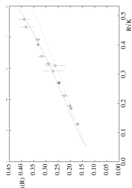
Figure 4: The effective running coupling constant $\alpha(R)$ obtained from the force between static quarks at separation $R$ from ref[9]. The scale is set by the string tension $K$. Data are at $\beta=6.5$ (diamonds) and at $\beta=6.2$ (triangles). The dotted error bars represent an estimate of the systematic error due to lattice artefact correction. The curves are the two-loop perturbative expression with $a(6.5)\Lambda_{R}=0.060$ (dotted) and 0.070 (continuous).

The figure clearly shows a running coupling constant. Moreover the result is consistent with the expected perturbative dependence on $R$ at small $R$. There are systematic errors, however. At larger $R$, the perturbative two-loop expression will not be an accurate estimate of the measured potentials, while at smaller $R$, the lattice artefact corrections (which arise because $R/a\approx 1$) are relatively big. Setting the scale using $\sqrt{K}=0.44$ GeV implies $1/a(\beta=6.5)=4.13$ GeV, so $R<4a(6.5)$ corresponds to values of $1/R>1$ GeV. This $R$-region is expected to be adequately described by perturbation theory.

This determination from the interquark force of the coupling $\alpha$ allows us to compare the result with the bare lattice coupling determined from $\beta=6/g^{2}$. At $\beta=6.5$, $\alpha_{\rm bare}=g^{2}/4\pi=0.073$. the values of $\alpha$ shown in fig 4 are much larger. The effective coupling constant is thus almost twice the bare coupling. This is quite acceptable in a renormalisable field theory. The message is that the bare coupling should be disregarded - it is not a good expansion parameter. The measured $\alpha$, however, proves to be a reasonable expansion parameter in the sense that the first few terms of the perturbation series converge. This successful calibration of perturbation theory on a lattice is important in practice. For instance, when matrix elements are measured on a lattice they have finite correction factors (usually called Z) to relate them to continuum matrix elements. These Z factors are evaluated perturbatively - so an accurate continuum prediction needs trustworthy perturbative calculations.

4 Full QCD

So far we have discussed the glueball spectrum, interquark potentials and $\alpha_{S}$ in the quenched approximation. This corresponds to treating the sea quarks as of infinite mass (so they don’t contribute to the vacuum). To make direct comparison with experiment, it is necessary to estimate the corrections from these dynamical quark loops in the vacuum.

The strategy is to use a finite sea-quark mass but still a value larger than the empirical light quark mass. The reason is computational: the algorithms become very inefficient as the sea-quark mass is reduced. The target is to study the effects as the sea-quark mass is reduced and then extrapolate to the physical value. The present situation, in broad terms, is that there is no significant change as the sea-quark mass is reduced. This could be because there are no corrections to the quenched approximation. Alternatively, the corrections may only turn on at a much lower quark mass than has been explored so far.

Let us try to make this argument a little more quantitative. For heavy sea-quarks of mass $m$, their contribution will be approximately proportional to $e^{-2m/E}$ where $E$ is a typical hadronic energy scale (a few hundred MeV). Thus the quark loop contributions will be negligible for $m>>E$, which corresponds to the quenched approximation. As $m\approx E$, the effects will turn on in a non-linear way.

The computational overhead of full QCD on a lattice is so large because the quark loops effectively introduce a long range interaction. The quark interaction in the Lagrangian is quadratic and so can be integrated out analytically. This leaves an effective Lagrangian for the gluonic fields which couples together the fields at all sites. This implies that, in a Monte Carlo method, a change in gluon field at one site involves the evaluation of the interaction with all other sites. In practice, one makes small changes at all sites in parallel, but this still amounts to inverting a large sparse matrix for each update. This is computationally slow.

As the sea-quark mass becomes small, one would expect to need a larger lattice size to hold the quarks. For heavy quarks, the effective range of the quark loops in the vacuum will be of order $1/m$. Thus the quenched approximation corresponds to $m\to\infty$ and a local interaction. For light quarks of a few MeV mass, the range will not be $1/m$, because quarks are confined. The lattice studies that have been made suggest that spatial sizes of order twice those adequate for the quenched approximation are needed for full QCD. This also implies considerable computational commitment.

A popular indication of how close a full QCD study is to experiment is to ask whether the $\rho$ meson can decay to two pions. Since the decay is P-wave, it needs non-zero momentum. On a lattice spatial momentum is quantised in units of $2\pi/L$. Thus we need $m_{V}>2m_{P}+2\pi/L$ for the decay channel to be allowed energetically. At present this criterion is rarely satisfied in quenched studies, let alone in the more computationally demanding case of full QCD.

The conclusion of current full QCD lattice calculations is that the expected sea-quark effects are not yet fully present. The main effect observed in full QCD calculations is that the lattice parameter $\beta$ which multiples the gluonic interaction term in the Lagrangian is shifted. Apart from this renormalisation of $\beta$, there is little sign of any other statistically significant non-perturbative effect.

Consider the changes to be expected for the inter-quark potential when the full QCD vacuum is used:

• At small separation $R$, the quark loops will increase the size of the effective coupling $\alpha$ compared to the pure gluonic case. This effect can be estimated in perturbation theory and the change at lowest order will be from 1/33 to 1/(33-$2N_{f}$).

• At large separation $R$, the potential energy will saturate at a value corresponding to two ‘heavy-quark mesons’. In other words, the flux tube between the static quarks will break by the creation of a $q\bar{q}$ pair from the vacuum.

Current lattice simulation [13] shows some evidence for the former effect but no statistically significant signal for the latter.

If one assumes that these lattice simulations are an approximation to the true full QCD vacuum, then one can use them to estimate the full QCD running coupling from lattice studies. A summary [10] of present lattice results is that

$$\alpha_{{\rm\overline{MS\kern-0.98pt}\kern 0.98pt}}(M_{Z})=0.112(7)$$

This conclusion will be reinforced when the full QCD lattice results reproduce more of the features of the experimental spectrum.

5 Quenched hadron masses

Since the full QCD simulation is not feasible at present, it is worthwhile to explore the hadron spectrum in the quenched approximation. This amounts to allowing quarks to propagate in the gluonic vacuum. Computationally this can be studied by solving the lattice Dirac equation for the quarks. Since the gluonic vacuum is full of rich structure, this is a computationally intensive problem: it amounts to inverting a large sparse matrix. Indeed it proves necessary to compute the quark propagation for a range of valence quark masses larger than the physical light quark masses and then extrapolate. Because of this, the statistical precision of such calculations is still somewhat limited. Nevertheless, different groups using different methods agree on the main results. For a recent review see ref[10].

Let us first discuss the $\rho$ meson. In fig 5, the mass is compared  [16] to a lattice scale (here $\Sigma=Ka^{2}$ where $K$ is the string tension). The figure shows that different treatments of fermions on the lattice (Wilson, Clover and staggered) with different discretisation errors ($a$, $\alpha_{S}a$ and $a^{2}$ respectively) are in agreement with a common continuum limit. Moreover, using the usual convention that the string tension is $\sqrt{K}=0.44$ GeV, the continuum value of $m_{\rho}/\sqrt{K}$ of 1.80(5) yields $m_{\rho}=0.79(2)$ GeV which is consistent with the experimental value of 0.77 GeV.

Studies have been made of the mesons and baryons which are composed of light and strange quarks- see ref[10]. The surprise is that the quenched approximation seems to reproduce these experimental values quite well. This may reflect the relatively large errors that are still present in the lattice determinations. It may also reflect the fact that the hadronic dynamics has a similar energy scale in each case so that the quenched approximation makes similar errors - which cancel in mass ratios.

Figure 5: The mass of the $\rho$ meson as a dimensionless ratio to the lattice string tension $\Sigma=Ka^{2}$. The continuum limit corresponds to $a\to 0$ at the left hand side. The filled squares are with staggered fermions, the open squares from Wilson fermions and the triangles are from Clover fermions. The lines show the discretisation errors which behave as $a^{2}$, $a$ and $\alpha_{s}a$ respectively.

6 Matrix elements eg $f_{P}$

Figure 6: The diagram representing a static quark Q propagating in the time direction and a light quark q which creates a gauge invariant quantity appropriate for studying $f_{B}$.

One of the advantages of lattice QCD is that it is a method to calculate hadronic matrix elements from first principles. Consider as an example the weak decay of a pseudoscalar meson P. The weak axial current will couple to the quarks in the meson. This current will be local. Thus the required quantity will relate the quark current to the hadronic state P. This is the pseudoscalar decay constant $f_{P}$ which is defined by the matrix element of the divergence of the axial current. For a pseudoscalar state of zero spatial momentum,

$$<0|q_{\mu}j^{A}_{\mu}|P>={f_{P}\over\sqrt{2m_{P}}}$$

where $j^{A}$ is the axial current which in terms of quark fields is $\bar{q}\gamma_{5}\gamma_{\mu}q$. For the pion, this identity is the partially conserved axial current (PCAC) relation and $f_{\pi}$ is the coupling of the pion to the weak current (and hence is relevant to the $\mu+\nu$ decay mode of the pion). Since the axial current is represented by local quark fields, $f_{P}$ gives a relationship between the hadronic state ($|P>$) and the quark sub-structure ($j^{A}$).

For a pseudoscalar meson with a heavy quark, such as the B meson, this same relationship is needed. Because the relevant weak decay is not currently observable (branching ratio too small), a lattice calculation is needed to determine $f_{B}$. The picture, for a heavy quark, is clarified by the heavy quark effective theory (HQET) which treats the heavy quark as slow moving. In the static limit, the lattice calculation needed is easily visualised. A straight line of colour flux of length $T$ in the lattice time direction represents the propagation of the heavy quark. By combining this with the propagator from one end to the other of a light quark in the lattice gluonic background field, one has a gauge invariant quantity which can be measured on a lattice (see fig 6). At each end, one joins the heavy quark to the light quark by a local axial current ($\gamma_{5}\gamma_{4}$ for a state at rest). Then the observed correlation $C(t)$ is proportional to $f_{P}^{2}e^{-E_{P}T}$ for large $T$ so allowing $f_{P}$ and $E_{P}$ do be determined in principle. In practice more sophisticated methods are used to improve the lattice measurement signal. Here $E_{P}$ has the interpretation of the mass difference of the B meson and the $b$ quark - although this difference is not directly useful since a non-perturbative definition of the quark mass requires careful discussion.

As well as using static quarks, lattice studies have been performed using propagating heavy quarks. Combining the results from both studies [16] yields $f_{B}=180(50)$ MeV. This value is needed as an ingredient in using experimental data to fix the CKM weak matrix elements. This is turn has implications for the experimental feasibility of CP violation through studies of $\bar{B}B$ mixing.

7 Outlook

Lattice techniques can extract reliable continuum properties from QCD. At present, the computational power available combined with the best algorithms suffices to give accurate results for many quantities in the quenched approximation. The future is to establish accurate values for more subtle quantities in the quenched approximation (eg. weak matrix elements of strange particles) and to establish the validity of the quenched approximation by full QCD calculations.

We need to reach the stage where an experimentalist saying ‘as calculated in QCD’ is assumed to be speaking of non-perturbative lattice calculations rather than perturbative estimates only.

References

- [1] P. De Forcrand, et al., Phys. Lett. 152B (1985) 107
- [2] C. Michael and M. Teper, Nucl. Phys. B314 (1989) 347
- [3] UKQCD collaboration, G. Bali, K. Schilling, A. Hulsebos, A. C. Irving, C. Michael and P. Stephenson, Phys. Lett. B309 (1993) 378-84.
- [4] H. Chen, J. Sexton, A. Vaccarino, and D. Weingarten, Nucl. Phys. B (Proc. Suppl.) 34 (1994) 357-359.
- [5] J. Sexton, A. Vaccarino, and D. Weingarten, Nucl. Phys. B (Proc. Suppl.) 42 (1995) 279.
- [6] G.S. Bali and K. Schilling, Phys. Rev. D47 (1993) 661; H. Wittig (UKQCD collaboration) Nucl. Phys. B (Proc. Suppl) 42 (1995) 288.
- [7] A. Billoire, Phys. Lett. 104B (1981) 472.
- [8] C. Michael, Phys. Lett. 283B (1992) 103.
- [9] UKQCD collaboration, A. Hulsebos et al., Phys. Lett. B294 (1992) 385.
- [10] C. Michael, Nucl. Phys. B (Proc. Suppl.) 42 (1995) 147-61.
- [11] G. P. Lepage and P. B. Mackenzie, Phys. Rev. D48 (1993) 2250.
- [12] C. Michael, G. A. Tickle and M. Teper, Phys. Lett. B 207 (1988) 313.
- [13] U. M. Heller et al.,Phys. Lett. B335 (1994) 71.
- [14] S. Perantonis and C. Michael, Nucl. Phys. B347 (1990) 854
- [15] C. Michael, Proc. of Aachen Workshop, ‘QCD 20 Years Later’, eds H. Kastrup and P. Zerwas, World Scientific 1993, pp 505-519.
- [16] R. Sommer, Nucl. Phys. B (Proc. Suppl.) 42 (1995) 186.