The Phase Diagram of Crystalline Surfaces

Abstract

We report the status of a high-statistics Monte Carlo simulation of non-self-avoiding crystalline surfaces with extrinsic curvature on lattices of size up to $128^{2}$ nodes. We impose free boundary conditions. The free energy is a gaussian spring tethering potential together with a normal-normal bending energy. Particular emphasis is given to the behavior of the model in the cold phase where we measure the decay of the normal-normal correlation function.

SU-HEP-95-4241-620

UFIFT-HEP-95-18

1 Introduction

In recent years there has been a lot of interest in the statistical mechanics of crystalline and fluid surfaces [1]. The former is believed to describe physical polymerized membranes [2] and the latter may be a regularization of string theory.

We focus our study on crystalline surfaces with bending rigidity embedded in $R^{3}$. It is conjectured that this model has a second order phase transition driven by the competition between entropy and the bending energy [3]. The high temperature phase is characterized by crumpled configurations. In the low temperature phase the system is no longer isotropic and the surfaces are roughly flat.

One may wonder what stabilizes the flat phase. The theoretical argument is that the in-plane elastic constants prevent the surface from fluctuating arbitrarily in the embedding space. This leads to an effective long wave stiffening of the surface [1, 3].

The crumpling transition has been studied numerically with simulations explicitly incorporating 2-d elastic constants [4, 5, 6]. There have also been simulations with a simple gaussian spring potential playing the role of the tethering potential [7, 8, 9, 10, 11, 12]. In both cases evidence has been presented for a continuous phase transition.

In the latter class of models the equilibrium spring length is taken to be zero, and a simple calculation indicates that the microscopic elastic constants vanish [13]. It is tempting to argue, therefore, that the flat phase of these models is not truly stable, even in the limit of large bending rigidity.

Our ultimate aim is to carefully compare the behavior of the appropriate observables in the cold phase as a function of the equilibrium spring length.

2 The Model

Consider a system of particles connected to form a triangular 2–d mesh embedded in 3 dimensions. Let each particle be labeled by an internal discrete coordinate system ${\bf x}=(x_{1},x_{2})$ denoting its position on the mesh. Its actual position in the embedding space is given by the 3 dimensional vector ${\bf r}(x_{1},x_{2})$. The action has a tethering potential and a bending energy term. Our choice is to use simple gaussian springs between the vertices as a tethering potential and a normal-normal interaction as the bending energy term. Therefore the action is

$$S=\sum_{\langle{\rm xx^{\prime}}\rangle}\left(l_{\rm xx^{\prime}}\right)^{2}+\lambda\sum_{\langle\alpha\beta\rangle}\left(1-\vec{n}_{\alpha}\cdot\vec{n}_{\beta}\right).$$ (1)

Here the subscripts ${\rm x,x^{\prime}}$ label the vertices and $l_{\rm xx^{\prime}}$ is the distance between the vertices ${\rm x}$ and ${\rm x^{\prime}}$ in the embedding space. The subscripts $\alpha,\beta$ label the faces (triangles) of the surface, $\vec{n}$ is the unit normal to the face and $\lambda$ is the bending rigidity. The sums extend to nearest neighbours. Eq. 1 describes phantom surfaces since it does not include self-avoidance. The surface is a rhombus with free boundaries cut out of a triangular lattice. In the case of a spring of length $a$, ($l_{\rm xx^{\prime}}$) has to be replaced by ($l_{\rm xx^{\prime}}-a$). In this case our model would closely resemble the one of [4] discussed above.

We focused our analysis on the following observables: the specific heat,

$$C_{v}=\frac{\lambda^{2}}{V}\left(\langle S_{e}^{2}\rangle-\langle S_{e}\rangle^{2}\right).$$ (2)

Here $S_{e}$ is the bending energy term considered above and $V$ is the total number of vertices.

The radius of gyration,

$$R_{g}^{2}=\frac{1}{3V}\langle\sum_{i}{\bf r}_{i}^{\prime}\cdot{\bf r}_{i}^{\prime}\rangle.$$ (3)

Here ${\bf r}_{i}^{\prime}$ is the position of the node $i$ in the embedding space referred to the center of mass. This observable measures the physical extent of the surface and its scaling behavior with system size defines the size (Flory) exponent $\nu$, via the relation $R_{g}\propto L^{\nu}$. The exponent $\nu$ is related to the Hausdorff dimension $d_{H}$ via the relation $\nu=2/d_{H}$.

The eigenvalues of the inertia tensor; these eigenvalues give information on the shape of the surface and how it scales with system size. They are obtained by diagonalizing the anisotropic part of the inertia tensor

$$A_{ab}=\sum_{i}{r}_{a}^{\prime}(i){r}_{b}^{\prime}(i)$$ (4)

where $a,b$ refer to the components of the vector ${\bf r^{\prime}}$.

The normal-normal correlation function,

$$G(R)=\langle\frac{1}{N}\sum_{|\alpha|=R}\left(\vec{n}_{\alpha}\cdot\vec{n}_{O}\right)\rangle.$$ (5)

Here the sum extends to all triangles of the surface which have a geodesic distance $R$ from the center of the surface $O$. The angle brackets represent the Monte-Carlo average.

Figure 1: The specific heat as a function of the bending rigidity.

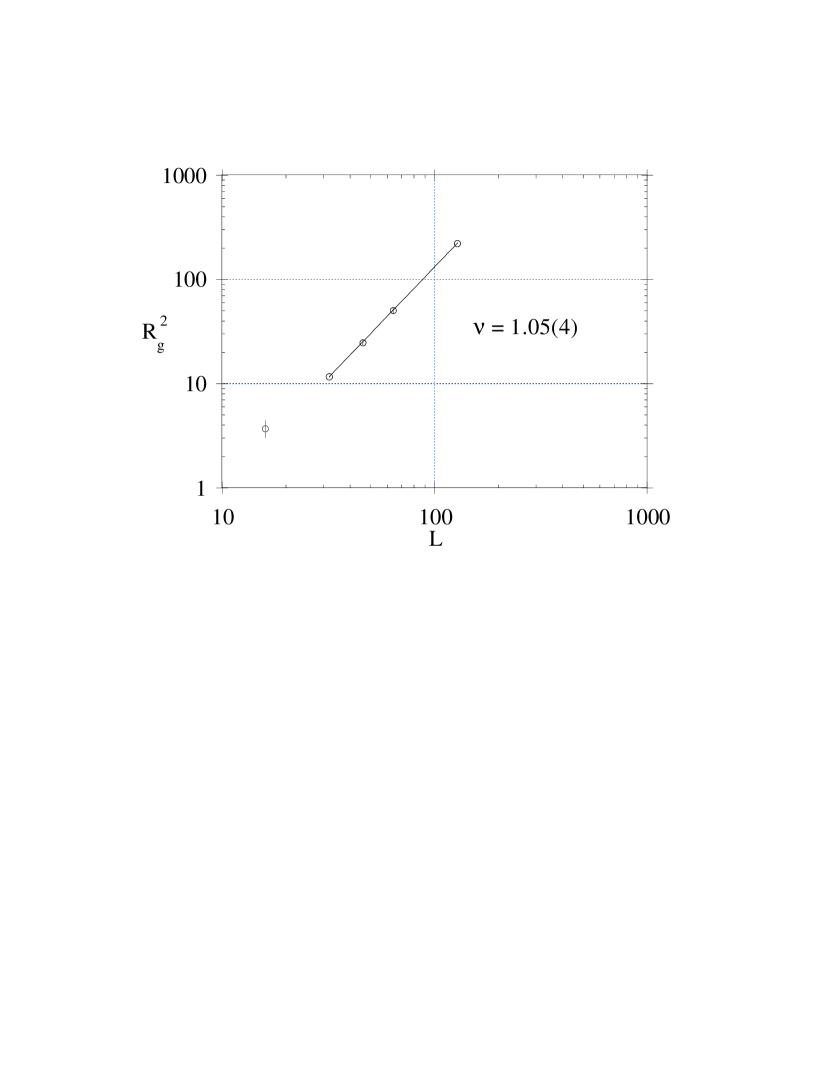
Figure 2: The scaling of the radius of gyration squared with system size in the cold phase($\lambda=1.1$). The fit gives a value of $\nu=1.05(4)$.

3 Theoretical Predictions

A self-consistent perturbation theory analysis of the continuum model [14] yields predictions for the critical exponents. The exponents of interest are the size (Flory) exponent $\nu$ and the roughness exponent $\xi$. The roughness exponent is defined by the scaling of the minimum eigenvalue of the inertia tensor (4),

$$\lambda\propto L^{2\xi}.$$ (6)

At the critical point the theory predicts $\nu~{}=~{}\xi~{}=~{}0.732$ while in the cold phase $\nu~{}=~{}1$ and $\xi~{}=~{}0.59$.

As far as the normal-normal correlation is concerned the only analytical result is for $\lambda=0$ (gaussian model). In this case the correlation function follows a decay law $G(R)\propto-1/R^{4}$.

4 Numerics and Results

We performed Monte-Carlo simulations of systems of sizes $16^{2}$ to $128^{2}$ vertices. We used the single hit Metropolis algorithm. The largest lattice was simulated on a MASPAR MP1 massively parallel processor, while all other sizes were simulated on workstations. We gathered statistics of the order of 30–50$\times 10^{6}$ sweeps per data point for the largest lattices (64 and 128). Our statistics are comparable for the smaller lattices.

As can be seen in Fig. 1 the specific heat $C_{v}$ shows a growing peak with system size. Presently our statistics are not yet sufficient to allow a reliable estimate of the exponent $\alpha$ which characterizes the growth. Preliminary fits indicate a value of $\alpha\approx 0.5$ consistent with the value obtained in [10, 11] using the same method. Our best estimate for the critical value of the coupling is around $\lambda\simeq 0.79$. Work is currently under way to gather better statistics and perform a Ferrenberg-Swendsen type analysis.

Fig. 2 shows the radius of gyration versus system size at a fixed value of $\lambda$ (1.1). The data fits well to a scaling ansatz with $\nu=1.05(4)$, as expected in the flat phase. In the crumpled phase the data does not fit a power law behavior, indicating, as expected [4, 5], a log-like scaling ($d_{H}=\infty$). Our estimate of the critical coupling is not precise enough to allow for a fit to $R_{g}$ at the transition.

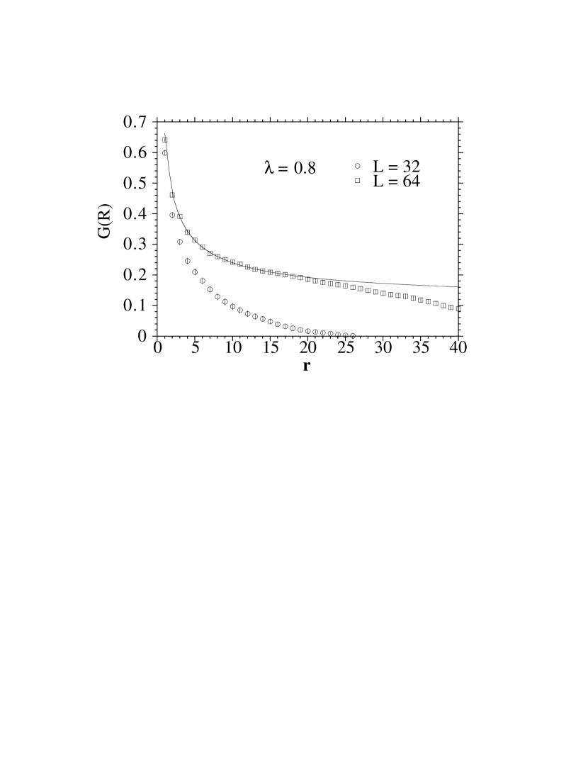
Figure 3: The normal-normal correlation function at $\lambda=0.8$ (around the phase transition).

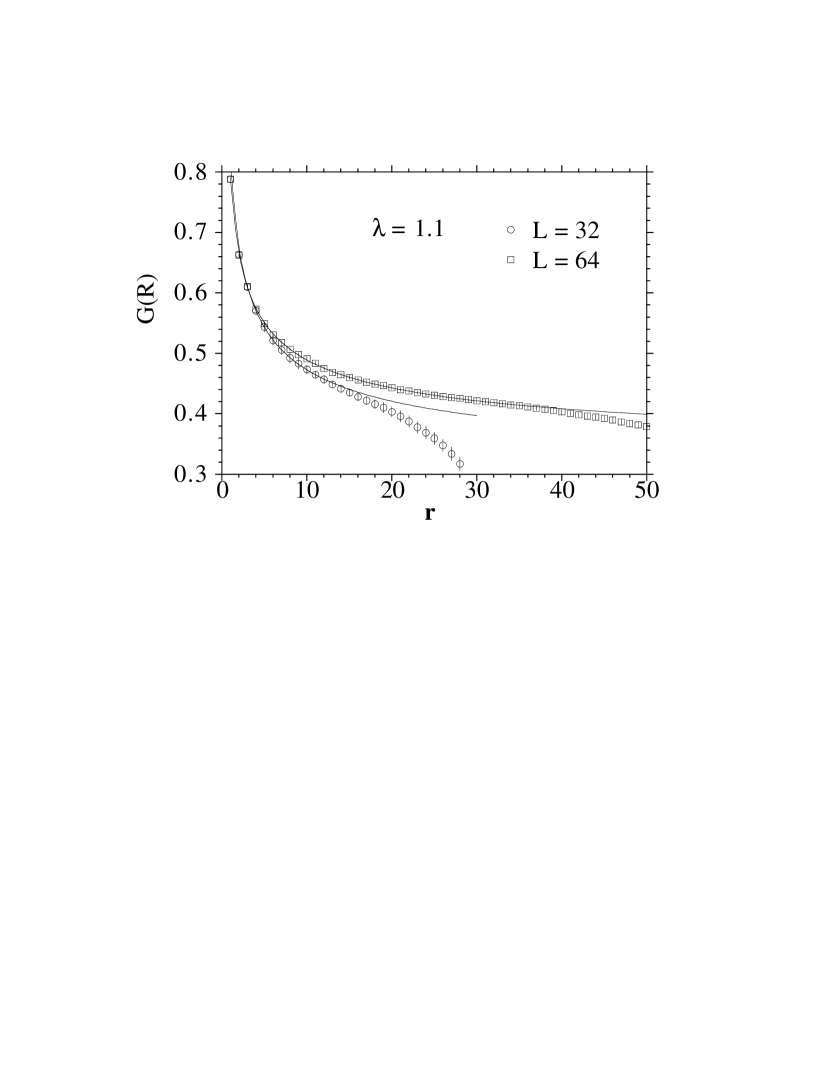
Figure 4: The normal-normal correlation function at $\lambda=1.1$ (in the cold phase).

Figures 3 and 4 show the normal-normal correlation around and above the phase transition respectively. Fig. 3 demonstrates the effect of finite-size corrections to the value of the critical coupling. For the smaller volume $L=32$ the correlation decays to zero with $r$, but fits indicate a non-zero asymptotic value for $L=64$. One possible reason is that, due to the volume dependence of the pseudo-critical coupling, the smaller volume is in the crumpled phase while the larger is in the cold (flat) phase. Note that for large $r$ the correlations will always decay to zero because of our choice of boundary conditions. This is a finite size effect and the data close to the boundary has to be excluded from the fits.

Figure 4 shows the correlation in the cold phase. The data for $L=64$ fits well to a behavior

$$G(R)\simeq\frac{1}{R^{a}}+b$$ (7)

with $a=0.51(1)$ and $b=0.3(1)$. Data for higher values of $\lambda$ and of the system size $L$ show a consistent behavior.

This is very important—the presence of a non-zero asymptote for the normal-normal correlation function indicates that the normals remain ordered on a macroscopic scale.

This result supports the existence of a stable flat phase. Our present focus is on the precise nature of this phase; in particular we would like to know if there is a well defined roughness exponent $\xi$ and if so how it depends on the bending rigidity. The existence of a flat phase with a roughness exponent independent of $\lambda$ would indicate that the entire flat phase $\lambda>\lambda_{c}$ is critical and that this model is in the same universality class as [15, 16, 17].

Another possibility is that the roughness exponent will depend on $\lambda$. In this case the flat phase would still be stable but not critical.

A possible interpretation of the stability of the flat phase is that the model discussed here dynamically generates a non-zero length scale which can serve to define non-zero renormalized elastic constants. This simple model could then be used to study the properties of physical (polymerized) membranes in regimes in which self-avoidance is irrelevant.

We are grateful for the use of NPAC computational facilities. The research of M.B. and M.F. was supported by the Department of Energy U.S.A. under contract No. DE-FG02-85ER40237. M.B. would also like to acknowledge support under NSF grant No. PHY89-04035 from the ITP at Santa Barbara, where some of this work was carried out. S.C. and G.T. were supported by research funds from Syracuse University. The research of K.A. was supported by the Department of Energy U.S.A.  under contract DE-FG05-86ER-40272. K.A. acknowledges IFT at Gainesville where part of this work was carried out.

References

- [1] “Statistical Mechanics of Membranes and Surfaces”, Vol. 5 of the Jerusalem Winter School for Theoretical Physics, D.R. Nelson, T. Piran and S. Weinberg eds., World Scientific, Singapore (1989). F. David, “Introduction to the Statistical Mechanics of Random Surfaces and Membranes”, in Vol. 8 of the Jerusalem Winter School for Theoretical Physics, D.J. Gross, T. Piran and S. Weinberg eds., World Scientific, Singapore (1992). Proceedings to the LXII Session of the Les Houches Summer School on “Fluctuating Geometries in Statistical Mechanics and Field Theory”, P. Ginsparg, F. David and C. Zinn-Justin eds., (URL http://xxx.lanl.gov/lh94).
- [2] C.F. Schmidt et al., Science 259 (1993) 952.
- [3] D.R. Nelson and L. Peliti, J. Phys. France 48 1987 (1085).
- [4] Y. Kantor and D.R Nelson, Phys. Rev. Lett. 58 (1987) 2774; Phys. Rev. A36 (1987) 4020.
- [5] Y. Kantor, M. Kardar and D.R. Nelson, Phys. Rev. Lett. 57 (1986) 791; Phys. Rev. A 35 (1987) 3056.
- [6] F.F. Abraham and D.R. Nelson, Science 249 (1990) 393.
- [7] J. Ambjørn, B. Durhuus and T. Jonsson, Nucl. Phys. B 316 (1989) 526.
- [8] M. Baig, D. Espriu and J. Wheater, Nucl. Phys. B 314 (1989) 587.
- [9] R. Renken and J. Kogut, Nucl. Phys. B 342 (1990) 753.
- [10] R.G. Harnish and J. Wheater, Nucl. Phys. B 350 (1991) 861.
- [11] J. Wheater and T. Stephenson, Phys. Lett. B 302 (1993) 447.
- [12] M. Baig, D. Espriu and A. Travesset, Nucl. Phys. B 426 (1994) 575.
- [13] D.R. Nelson, private discussion.
- [14] P. Le Doussal and L. Radzikovsky, Phys. Rev. Lett. 69 (1992) 1209.
- [15] J.A. Aronovitz and T.C. Lubensky, Phys. Rev. Lett. 60 (1988) 2634.
- [16] E. Guitter, F. David, S. Leibler and L. Peliti, Phys. Rev. Lett. 61 (1988) 2949; J. Phys. France 50 (1989) 1787.
- [17] J.A. Aronovitz, L. Golubovic and T.C. Lubensky, J. Phys. France 50 (1989) 609.