Coupling the Deconfining and Chiral Transitions

Abstract

The Polyakov loop and the chiral condensate are used as order parameters to explore analytically the possible phase structure of finite temperature QCD. Nambu-Jona-Lasinio models in a background temporal gauge field are combined with a Polyakov loop potential in a form suitable for both the lattice and the continuum. Three possible behaviors are found: a first-order transition, a second-order transition, and a region with both transitions.

1 INTRODUCTION

Our recent work[1] on an effective action for dynamical quarks has caused us to examine the simple picture in which deconfinement and chiral symmetry are independent. On the basis of this work, it appears necessary to consider models of the deconfining and chiral symmetry transitions in which the two order parameters, the chiral condensate and the Polyakov loop, are coupled.

In this paper we study a two flavor Nambu-Jona-Lasinio model [2] in a uniform background temporal gauge field with a Euclidean action of the form

$${\cal L}=\bar{\Psi}(D\!\!\!\!/\,+m)\Psi+G\left[(\bar{\Psi}\Psi)^{2}+(\bar{\Psi}i\gamma_{5}\vec{\tau}\Psi)^{2}\right]$$ (1)

where

$$D_{\mu}=\partial_{\mu}+igA_{\mu}(x)\quad{\rm with}\quad A_{\mu}(x)=\delta_{0\mu}A_{0}.$$ (2)

The spontaneous breakdown of $Z_{3}$ symmetry induced by the gauge field is modeled by a simple potential with cubic and quartic terms. Combined with the quark interaction effects, this model explicitly constructs a free energy dependent on the two order parameters, in the spirit of Landau-Ginsberg arguments. Because this model generates an effective potential consistent with two-flavor QCD, we will show that the class of critical behaviors possible in finite temperature QCD is a priori larger than has been previously realized.

2 EFFECTIVE POTENTIAL FOR FINITE TEMPERATURE NJL MODEL

We let $S_{0}$ denote the propagator for a free fermion with current mass $m$ and $S$ denote the propagator for a fermion with constituent mass $M$. Following Cornwall, Jackiw, and Tomboulis [3], a one-loop effective action $\Gamma(S)$ for the theory given in Eq. (1) at finite temperature is given by

$$\Gamma(S)={\rm Tr}\left[\ln\left(S_{0}^{-1}S\right)\right]-{\rm Tr}\left(S_{0}^{-1}S-1\right)$$

$$\quad\quad\quad\quad-\tilde{G}\int_{0}^{\beta}dt\int d^{3}\vec{x}\left[{\rm Tr}S(x,x)\right]^{2}$$ (3)

where $\tilde{G}=[1+1/(2N_{f}N_{c})]G$. The effective potential can be conveniently written in terms of the constituent mass M:

$$V(M,T)={(M-m)^{2}\over 4\tilde{G}}$$

$$-{2N_{f}\over\beta}\sum_{k_{0}}\int{d^{3}\vec{k}\over(2\pi)^{3}}{\rm tr_{c}}\ln\Bigl{[}(k_{0}+gA_{0})^{2}+\omega_{\vec{k}}^{2}\Bigr{]}$$ (4)

where $\omega_{\vec{k}}=\sqrt{\vec{k}^{2}+M^{2}}$. Evaluating the mode sum over $k_{0}$, we find that up to an irrelevant constant

$$V(M,T)={(M-m)^{2}\over 4\tilde{G}}-2N_{f}N_{c}\int{d^{3}\vec{k}\over(2\pi)^{3}}\omega_{\vec{k}}$$

$$+{2N_{f}\over\beta}\int{d^{3}\vec{k}\over(2\pi)^{3}}{\rm tr_{c}}\ln\left(1+e^{-\beta\omega_{\vec{k}}}{\cal P}\right)$$

$$+{2N_{f}\over\beta}\int{d^{3}\vec{k}\over(2\pi)^{3}}{\rm tr_{c}}\ln\left(1+e^{-\beta\omega_{\vec{k}}}{\cal P}^{\dagger}\right),$$ (5)

where ${\cal P}=e^{i\beta gA_{0}}$ is the Polyakov loop associated with the background $A_{0}$.

We regulate $V(M)$ by introducing a non-covariant cut-off, $\theta(\Lambda^{2}-\vec{k}^{2})$, and make the approximation

$${\rm tr_{c}}({\cal P}^{n})\approx N_{c}\left({{\rm tr_{c}}{\cal P}\over N_{c}}\right)^{n}.$$ (6)

Noting that the quark determinant forces the trace of the Polyakov loop to be real, Eq. (5) now becomes

$$V(M,T)={(M-m)^{2}\over 4\tilde{G}}-{N_{f}N_{c}\over\pi^{2}}\int_{0}^{\Lambda}dk\,k^{2}\omega_{k}$$

$$+{2N_{f}N_{c}\over\pi^{2}\beta}\int_{0}^{\Lambda}dk\,k^{2}\ln\Bigl{[}1+e^{-\beta\omega_{k}}\left({{\rm tr_{c}}{\cal P}\over N_{c}}\right)\Bigr{]}.$$ (7)

We determine $\Lambda$, $M$, and $\tilde{G}$ by simultaneously fixing the chiral condensate and the pion form factor [4], with $<\bar{\Psi}\Psi>=N_{f}(246.7MeV)^{3}$ and $f_{\pi}=93MeV$. For the remainder of this paper we will use the numerical solution [4, 5]

$$M=335.1MeV\qquad\Lambda=630.9MeV$$

$$\tilde{G}\Lambda^{2}=2.196,$$ (8)

which assumes a current quark mass $m_{u}=m_{d}=4MeV$.

3 POLYAKOV LOOP POTENTIAL

We denote $tr_{c}{\cal P}$ by $\phi$. Near the deconfinement temperature $T_{D}$ the potential of Polyakov loops in pure QCD can be approximated by a polynomial potential of the form [6]

$$U(\phi,T)=\lambda\left(\phi-{\phi^{2}\over\phi_{D}}\right)^{2}-{T-T_{D}\over T_{D}L^{-1}}\left({\phi\over\phi_{D}}\right)^{3}$$ (9)

The potential is parametrized such that for a pure gauge theory the phase transition occurs at $T_{D}$ with a latent heat $L$ and the Polyakov loop jumping from $0$ to $\phi_{D}$.

This choice for $U$ is phenomenological. Although perturbative QCD does yield a quartic polynomial potential for the $A_{0}$ field, the potential so obtained does not display critical behavior, and it is only valid at high temperatures [7]. However, it does suggest that the parameter $\lambda$ should be taken to be on the order of $T_{D}^{4}$. We have chosen $\lambda=T_{D}^{4}$ and $L=2T_{D}^{4}$ for the numerical calculations below, neglecting any possible temperature corrections or other dependencies in $\lambda$, $T_{D}$, $\phi_{D}$ and $L$. The direct association of $T_{D}$, $\phi_{D}$ and $L$ with measureable quantities holds only for very heavy quarks. For light quarks, these parameters must be determined by fitting to the observed behavior.

We can now couple the chiral symmetry and deconfinement phase transitions. Let

$${\cal V}(M,\phi,T)=V(M,\phi,T)+U(\phi,T),$$ (10)

where $V(M,\phi,T)$ is given in Eq. (7) with ${\rm tr_{c}}{\cal P}=\phi$. To determine the critical behavior of the coupled effective potential, the absolute minimum of the potential ${\cal V}(M,\phi,T)$ as a function of $M$ and $\phi$ must be found as $T$ is varied. A satisfactory determination of the entire phase diagram requires numerical investigation.

4 RESULTS

The two flavor Nambu-Jona-Lasinio model has a second-order chiral phase transition for massless quarks. For the parameter set used here, this transition occurs at $T_{\chi}=194.6$ MeV, as determined numerically from $V(M,\phi\equiv 1,T)$. The order of the transition is consistent with Monte Carlo simulations of two-flavor QCD, and the critical temperature is plausible. However, the finite temperature quark determinant is not consistent with the known behavior of QCD unless the effects of a non-trivial Polyakov loop are included. As Eq. 5 makes clear, the effects of finite temperature in the quark determinant are suppressed by the small expected value of the Polyakov loop at low temperatures. Without the Polyakov loop effects, the conventional Nambu-Jona-Lasinio model displays the $T^{4}$ behavior of a free quark gas at arbitrarily low temperatures.

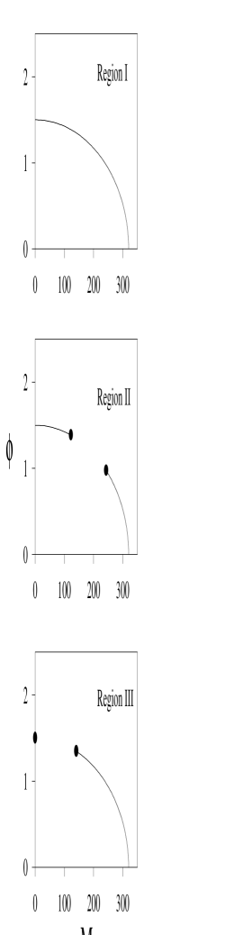
Figure 1: Schematic behavior of $\phi$ and $M$ in the three regions of the $(T_{D},\phi_{D})$ plane as temperature increases.

Numerical investigation shows that the critical behavior of ${\cal V}(M,\phi,T)$ is most sensitive to $T_{D}$ and $\phi_{D}$. Figure 1 illustrates the three distinct types of critical behavior observed as $T_{D}$ and $\phi_{D}$ are varied with the other parameters held fixed and the current mass $m$ set to $0$. In Region I of the $(T_{D},\phi_{D})$ plane the effective quark mass changes continuously from its $T=0$ value to a mass of $0$ MeV as the temperature increases, signaling a second-order chiral phase transition. Simultaneously, the expectation value of the trace of the Polyakov loop increases smoothly with temperature, exhibiting a large, but continuous, increase in the vicinity of the chiral transition. This region exhibits behavior most similar to that observed in simulations of two-flavor QCD. In Region II the Polyakov loop experiences a first-order jump at some $T_{c}$. At the same $T_{c}$ the constituent quark mass undergoes a sudden drop, but chiral symmetry is not restored. As the temperature increases beyond $T_{c}$, the constituent mass moves continuously to zero. Thus, there are two distinct phase transitions in Region II, a first-order transition driven by the dynamics of deconfinement, and a later second-order chiral symmetry restoring transition. In Region III the Polyakov loop experiences a first-order jump at some $T_{c}$, and simultaneously the effective quark mass drops suddenly to $0$ MeV, indicating a single first-order transition which restores chiral symmetry.

Figure 2 shows the location of the three regions in the $(T_{D},\phi_{D})$ plane. Figure 3 plots the behavior of the Polyakov loop, $\phi$, and the constituent quark mass, $M$, as a function of temperature at the point $(T_{D}=220{\rm MeV},\phi_{D}=1.2)$ in Region II. There is a clear separation of the first and second-order transitions.

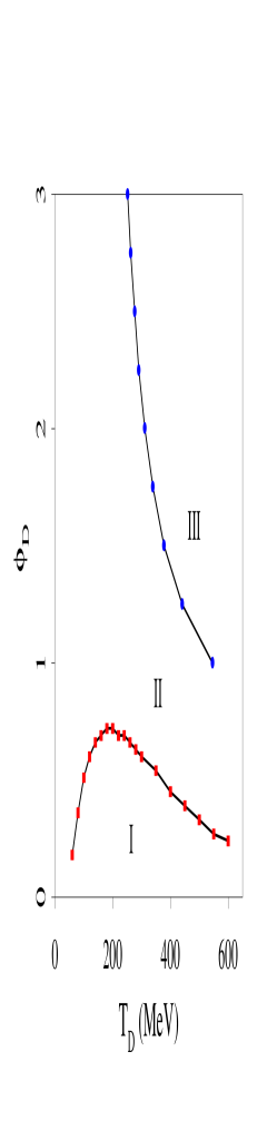
Figure 2: Phase diagram in the $(\phi_{D},T_{D})$ plane.

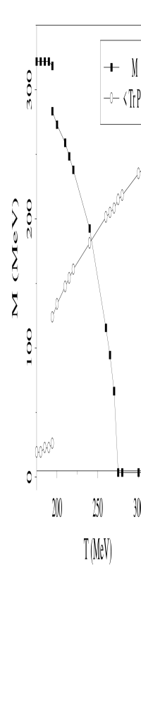
Figure 3: Plot of $\phi$ and $M$ as a function of temperature at the point $(T_{D}=220{\rm MeV},\phi_{D}=1.2)$ in Region II.

5 LATTICE VERSION OF THE EFFECTIVE POTENTIAL

A lattice version of the effective potential has the advantage that many parameters can be set from QCD simulations. There are two related issues in extending our work to the lattice: the choice of a lattice fermion formalism and setting other parameters in the effective action.

A lattice version of the NJL model can be straightforwardly implemented using naive fermions [8]. Species doubling can be handled by a formal replacement of $N_{c}$ with $N_{c}/16$. Using the single quark current mass, chiral condensate, and constituent mass of the last section as inputs, we find

$$a^{-1}=389.0MeV\qquad\tilde{G}a^{-2}=0.8343.$$ (11)

Hence, $f_{\pi}=94.09$ $MeV$. Also note that $M_{T=0}a$ is of order 1. The temperature is given by $T=1/(N_{t}a)$ where $N_{t}$ is the temporal extent of the lattice. This places a problematic upper limit on a discrete range of available temperatures. Given our choice of parameters, $T_{max}$ is only $194.5$ $MeV$.

The temperature may be changed continuously by an asymmetric rescaling of the lattice in which the lattice spacing $a_{t}$ in the temporal direction varies independently of the spatial lattice spacing $a_{s}$ [9]. Defining $a_{s}=a$ and $\xi=a_{t}/a_{s}$, we now have in physical units $T=1/(N_{t}a\xi)$. The effective potential is

$$V(M,\phi,\xi)=$$

$$-{N_{f}N_{c}\over 4\xi}\int_{-\pi}^{\pi}{d^{3}\vec{k}\over(2\pi)^{3}}\rm{ln}\left[\sqrt{1+{\xi}^{2}A^{2}(\vec{k})}+\xi A(\vec{k})\right]$$

$$-{N_{f}N_{c}\over 2N_{t}\xi}\int_{-\pi}^{\pi}{d^{3}\vec{k}\over(2\pi)^{3}}\rm{ln}\Bigl{\{}1+\Bigl{[}\sqrt{1+{\xi}^{2}A^{2}(\vec{k})}$$

$$-\xi A(\vec{k})\Bigr{]}^{N_{t}}{tr_{c}(\phi)\over N_{c}}\Bigr{\}}+{(M-m)^{2}\over 4\tilde{G}}$$ (12)

where $A(\vec{k})=\sqrt{M^{2}+\sum_{j}{\sin}^{2}(p_{j})}$. However, using the same inputs as the symmetric lattice case, as well as $f_{\pi}=93$ $MeV$, we find the unique answer

$$a^{-1}=477.2MeV\qquad\tilde{G}a^{-2}=1.255$$ (13)

with $\xi=2.002$.

An alternative to asymmetric lattices might be variant or improved actions for which $a^{-1}$ is larger.

6 CONCLUSION

Polyakov loop effects have a strong impact on the possible critical behavior of the NJL model. The universality argument [10] which predicts a second-order chiral transition for two flavors and a first-order transition for three or more flavors may fail when this additional order parameter is included.

References

- [1] P. N. Meisinger and M. C. Ogilvie, Nucl. Phys. B (Proc. Suppl.) 42, 532 (1995); P. N. Meisinger and M. C. Ogilvie, to be published in Phys. Rev. D
- [2] J. Nambu and G. Jona-Lasinio, Phys. Rev. 122, 345 (1961); J. Nambu and G. Jona-Lasinio, Phys. Rev. 124, 246 (1961)
- [3] J. M. Cornwall, R. Jackiw, and E. Tomboulis, Phys. Rev. D 10, 2428 (1974)
- [4] V. Bernard, Phys. Rev. D 34, 1601 (1986)
- [5] V. Bernard, U. G. Meissner, and I. Zahed, Phys. Rev. D 36, 1601 (1987); T. Hatsuda and T. Kunihiro, Prog. Theor. Phys. Supplement 91, 284 (1987); T. Meissner, E. R. Arriola, and K. Goeke, Z. Phys. A 336, 91 (1990)
- [6] T. Trappenberg and U. J. Wiese, Nucl. Phys. B372, 703 (1992)
- [7] N. Weiss, Phys. Rev. D 24, 475 (1981); N. Weiss, Phys. Rev. D 25, 2667 (1982)
- [8] K. M. Bitar and P. M. Vranas, Phys. Rev. D 50, 3406 (1994)
- [9] F. Karsch, Nucl. Phys. B205, 285 (1982)
- [10] R. D. Pisarski and F. Wilczek, Phys. Rev. D 29, 338 (1984)