HLRZ 56/95 hep-lat/9509040 Magnetic and chiral universality classes in a 3D Yukawa model

Abstract

The 3D Yukawa model with U(1) chiral symmetry is investigated in a broad interval of parameters using the Binder method. Critical exponents of the Wilson-Fisher (magnetic) and Gross-Neveu (chiral) universality classes are measured. The model is dominated by the chiral universality class. However at weak coupling we observe a crossover between both classes, manifested by difficulties with the Binder method which otherwise works well.

1 Introduction

The existence of nontrivial fixed points in 4D is not yet ruled out in nonperturbative calculations. Several gauge theories have, in addition to the Gaussian fixed points, also suspicious critical points at strong coupling. One of the purposes of our investigation of the 3D Yukawa model (Y₃) was to learn how to deal with models having several nontrivial fixed points and crossovers between the corresponding universality classes.

The Y₃ model is known to have two nontrivial fixed points: the Wilson–Fisher fixed point of the pure scalar $\phi_{3}^{4}$ theory at vanishing Yukawa coupling with a magnetic type phase transition, and the fixed point of the 3D Gross–Neveu model (GN₃) with a chiral phase transition.

The model is also interesting from the point of view of statistical mechanics. Transitions between different universality classes have been investigated in spin models [1] but not yet in fermionic ones. The most promising method used is Binder’s method of finite size scaling analysis. We have applied this method succesfully to the chiral phase transition. The failure of this method also indicates the occurence of a crossover to the magnetic universality class. The existence of intermediate universality classes between the two, corresponding to the known fixed points, is also of interest [1], but in the Y₃ model we didn’t detect any signs for it.

2 Lattice action and phase diagram

We studied the Y₃ model on the lattice with staggered fermions, hypercubic Yukawa coupling and U(1) chiral symmetry. The action is

$$S = \sum_{x}\left[-2\kappa\sum\limits_{\mu}\phi_{x+\mu}^{i}\phi_{x}^{i}+\phi_{x}^{2}+\lambda(\phi_{x}^{2}-1)^{2}\right.$$ (1)

$$+ \frac{1}{2}\sum\limits_{\mu}\eta_{x,\mu}(\overline{\chi}_{x}^{j}\chi_{x+\mu}^{j}-\overline{\chi}_{x+\mu}^{j}\chi_{x}^{j})$$

$$+ \left.y\overline{\chi}_{x}^{j}\frac{1}{2^{3}}\sum\limits_{b}(\phi_{x+b}^{1}+i\varepsilon_{x}\phi_{x+b}^{2})\chi_{x}^{j}\right]\>.$$

The staggered sign factors are $\eta_{x,1}=1$, $\eta_{x,\mu}=(-1)^{x_{1}+\ldots+x_{\mu-1}}$ and $\varepsilon_{x}=(-1)^{x_{1}+\ldots+x_{d}}$. The indices $x+\mu$ and $x+b$ denote, respectively, the nearest neighbors of the site $x$ and the corners of the associated elementary cube. The scalar field $\phi_{x}$ is a two component real field.

From considerations of the effective potential to 1-loop order and numerical simulations we determined the phase diagram sketched in fig. 1. It has two well-known limits: the $\phi_{3}^{4}$ model at $y=0$ and the GN₃ model at $\lambda=0$, $\kappa=0$. The region below the critical surface is the paramagnetic phase (PM), the region above the ferromagnetic phase (FM). For negative values of the parameter $\kappa$ we further expect an antiferromagnetic phase (AFM) and a ferrimagnetic phase (FI).

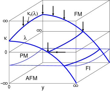
Figure 1: Sketch of the Y₃ phase diagram.

3 Numerical methods

For the numerical simulation we used a hybrid Monte-Carlo program. Ferrenberg-Swendsen multihistogram reweighting was used to interpolate between the measured points in the parameter space.

In order to find an appropriate method to identify the universality class corresponding to a certain critical point we tried several methods to compute critical exponents in the pure scalar limit of the model ($y=0$). The direct method using the scaling laws of the physical quantities and the method using the Lee–Yang zeros of the partition function needed significantly more statistics compared to Binder’s method of finite size scaling analysis of cumulants. Thus we used only the Binder method in the fermionic case, with the following definition for the cumulant:

$$U_{L}=2-\frac{\sum\limits_{x_{1},\dots,x_{4}}\sum\limits_{i,j}\langle\phi_{x_{1}}^{i}\phi_{x_{2}}^{i}\phi_{x_{3}}^{j}\phi_{x_{4}}^{j}\rangle}{(\sum\limits_{x_{1},x_{2}}\sum\limits_{i}\langle\phi_{x_{1}}^{i}\phi_{x_{2}}^{i}\rangle)^{2}}{}~{}.$$ (2)

The validity of the hyperscaling hypothesis implies that these cumulants are independent of the lattice size at the critical point. This is a very precise way of determining critical couplings.

Critical exponents can be computed by considering pairs $(bL,L)$ of lattice sizes. The cumulants deliver the exponent $\nu$ of the scalar correlation length $\xi$:

$$\ln\frac{\partial U_{bL}}{\partial U_{L}}\bigg{|}_{\kappa_{c}}=\frac{1}{\nu}\ln b\;.$$ (3)

Similarly we obtained $\gamma/\nu$ and $\beta/\nu$ from the susceptibility $\chi_{L}$ and the magnetization $M_{L}$.

4 The $\phi_{3}^{4}$ model

The action (1) describes at vanishing $y$ free massless fermions and $O(2)$ invariant scalars with selfinteraction ($\phi_{3}^{4}$ model). We have determined the phase diagram of this model (for the data see [2]). At positive $\kappa$ a critical line of second order phase transitions $\kappa_{c}(\lambda)$ separates the PM and FM phases. At the point $\kappa_{c}(\lambda=0)$ the theory is dominated by a Gaussian fixed point, being asymptotically free at large momenta. All other points on the critical line $\kappa_{c}(\lambda>0)$ lead to a nontrivial continuum limit, dominated by the Wilson–Fisher fixed point. In order to test this expectation, we measured the renormalized quartic coupling and the critical exponents $\nu$, $\beta/\nu$ and $\gamma/\nu$ at two values of the bare scalar quartic coupling: $\lambda=0.5$ and $\lambda=\infty$. Fig. 3a illustrates the quality of determination of $\kappa_{c}$ by the Binder method at $\lambda=\infty$. These measurements helped us to develop and test the methods later used for nonvanishing $y$.

The renormalized scalar quartic coupling

$$\lambda_{R}=(Lam_{R})^{3}U_{L}$$ (4)

has been determined by keeping the ratio $L/\xi$ fixed to $4$ and varying the lattice size $L$ between $6$ and $12$. The extrapolation to infinite volume suggests $\lambda_{R}=26(4)$ for both values of $\lambda$.

The critical exponents we calculated by the Binder method are summarized in the following table.

$\lambda$	$\kappa_{c}$	$\nu$	$\beta/\nu$	$\gamma/\nu$
$\infty$	0.2275(10)	0.673(19)	0.51(3)	2.03(6)
0.5	0.241(1)	0.687(19)	0.56(5)	1.91(6)

The results are consistent within error bars and also with the hyperscaling hypothesis. They confirm that the continuum limits at $\lambda=\infty$ and $\lambda=0.5$ belong to the Wilson–Fisher universality class.

5 Y₃ model at $\lambda=0$

The GN₃ model with $U(1)$ chiral symmetry arises in the limit $\lambda=0$. It is renormalizable in the $1/N_{F}$ expansion and its $\beta$ function has been calculated up to $O(1/N_{F}^{2})$ [3]. The critical exponent $\nu$ resulting from these calculations is $\nu\simeq 1.0(1)$.

The phase structure of the GN₃ model can be read of fig. 1. The symmetric phase ($y<y_{c}$), where fermions are massless, is dominated by the Gaussian fixed point at $y=0$. The critical point $y_{c}=1.091(5)$ is an UV stable nontrivial fixed point.

Figure 2: Determination of the critical exponent $\nu$ in the Gross–Neveu.

We applied the Binder method to the GN₃ model. We approached the critical point both by varying $y$ at $\lambda=\kappa=0$ (GN case) and $\kappa$ at $\lambda=0$ and $y=y_{c}$. Fig. 2 shows the determination of $\nu$ using eq. (3). Fig. 3b shows that the cumulants cross in the GN case at $y=1.091$. The obtained exponents are perfectly consistent with each other and the theoretical values. Their averages are: $\nu=1.03(10)$, $\beta/\nu=0.89(7)$, $\gamma/\nu=1.17(9)$, values which are significantly different from the Wilson–Fisher exponents and allow the investigation of crossover effects between these universality classes.

Figure 3. Determination of $\kappa_{c}$: (a) in the XY₃ model, (b) in the GN₃ model and (c) at $\lambda=\infty$, $y=0.6$. It works well in the first two cases, but only poorly in the third case.

6 Y₃ model at $\lambda=\infty$

There are theoretical arguments [4] which predict that Y₃ and GN₃ models belong to the same universality class for small values of $\lambda$. We tested this conjecture for $\lambda=\infty$ by determining the critical exponents at large Yukawa coupling ($y=1.1$).

The Binder method works as well as in the GN₃ case. At $y=1.1$ and $\lambda=\infty$ we varied $\kappa$ and determined first its critical value. The intersection point of the cumulants on different lattice sizes delivers with good accuracy $\kappa_{c}=0.007(2)$. Using eq. (3) the critical exponent $\nu$ has been extracted: $\nu=0.89(6)$. Further we determined: $\beta/\nu=0.80(8)$ and $\gamma/\nu=1.30(7)$.

All these exponents are consistent with those of the GN₃ fixed point and significantly different from the Wilson–Fisher exponents. We conclude that, at least for strong enough Yukawa coupling, the critical surface from $\lambda=0$ to $\lambda=\infty$ belongs to the GN universality class.

At $\lambda=\infty$ but smaller Yukawa coupling crossover phenomena make the determination of critical exponents more difficult.

At $y=0.6$ it is difficult to determine $\kappa_{c}$ (fig. 3c). For small lattices ($L=6,8,10$) the cumulants cross in the interval $\kappa=0.146-0.1466$. The finite size analysis delivers $\nu=0.79(9)$, inconsistently to the GN universality class. When only lattices larger than $L=10$ are considered, the crossing point of the cumulants is $\kappa_{c}\simeq 0.144$. An analysis for this $\kappa_{c}$ leads to $\nu=0.99(23)$. This value is consistent with the GN critical exponent. The reason for the strong dependence of the calculated $\nu$ on $\kappa_{c}$ is a larger curvature in the functions $U_{bL}(U_{L})$. Thus the value of the derivative $\partial U_{bL}/\partial U_{L}$ depends stronger on the value of $\kappa_{c}$ than in the $\phi_{3}^{4}$ and strong $y$ cases.

The computations at $y=0.3$ revealed even stronger crossover effects. Though lattices up to $L=32$ have been used, the value of $\kappa_{c}$ couldn’t be determined. A very strong curvature in $U_{bL}(U_{L})$ makes an accurate calculation of $\nu$ impossible on such small lattices.

7 Boson mass in the Y₃ model

In the Gross–Neveu model the bosonic particles can be interpreted as fermion-antifermion bound states, because the scalar field introduced in the action is auxilliary. In the full Yukawa model and its purely scalar limit $\phi_{3}^{4}$ the $\phi$ field is dynamical. We measured the propagator of the two components of the $\phi$ field in momentum space. While in the $\phi_{3}^{4}$ model this propagator can be fitted with a free boson Ansatz, its form is very complex at nonvanishing Yukawa coupling. We were able to fit it with an Ansatz using renormalized lattice perturbation theory.

Fig. 4 shows such a bosonic propagator in the Gross–Neveu case and the fit. The characteristic form, which is reproduced well by the fit, is the same for all $\lambda$ values, including $\lambda=\infty$. Also the behavior of the boson mass across the phase transition is very similar both at $\lambda=0$ and $\lambda=\infty$. This is another piece of evidence that the Y₃ and GN₃ models are equivalent (belong to the same universality class).

Figure 4: Bosonic propagator in the GN₃ model at $\lambda=\kappa=0$, $y=1.1$.

References

- [1] M. D’Onorio De Meo, J.D. Reger and K. Binder, Physica A (1995) in print.
- [2] E. Focht, J. Jersák and J. Paul, preprint Jülich HLRZ 46/95.
- [3] J.A. Gracey, Phys. Rev. D50 (1994) 2840.
- [4] J. Zinn-Justin, Nucl. Phys. B367 (1991) 105.