BU-CCS-950601
BROWN-HET-999 hep-lat 9509012
MIT-CTP-2461

Chronological Inversion Method for the Dirac Matrix

in Hybrid Monte Carlo

R.C. Brower⁽¹⁾, T. Ivanenko⁽²⁾, A.R. Levi⁽¹⁾ and K.N. Orginos⁽³⁾

⁽¹⁾Department of Physics, Boston University, Boston, MA 02215, USA

⁽²⁾Center for Theoretical Physics, Mass. Inst. of Tech., Cambridge, MA 02139, USA

⁽³⁾Department of Physics, Brown University, Providence, RI 02912, USA

I. Introduction

At present, typical methods for going beyond the quenched (or valence) approximation for lattice QCD involve an increase of several orders of magnitude in computational time — severely limiting statistics on large lattices. Consequently, finding a more efficient approach to the inclusion of internal fermion loops poses a major challenge for the next generation of lattice simulations [1].

The most successful approach to date for generating full QCD configurations is the so-called Hybrid Monte Carlo (HMC) algorithm [2], which uses Molecular Dynamic (MD) evolution in a “fifth time” coordinate t. At each time step, the Dirac matrix must be inverted to calculate the force due to fermion loops. This inversion is the most time-consuming part of the full QCD algorithm. The Dirac operator is represented as a $12V$ by $12V$ sparse square matrix, where the number of space-time lattice sites (or volume $V$) is on the order of $10^{5-6}$. With the lattice volumes used in recent simulations, the Dirac matrix may account for 90% or more of the computer’s time. Moreover, due to the Dirac inverter, the problem scales as $(1/a)^{6-7}$. Therefore any acceleration of the Dirac inversion implies a major improvement in the overall performance of generating QCD configurations.

Our simple observation is that by virtue of the system’s smooth evolution in MD time, it should be possible to use information from the recent past to perform the next inverse more efficiently [3].

Our present approach to make use of the past data is straightforward [4]. Since the conjugate gradient is an iterative procedure, a trial starting configuration is needed. Our method is to “extrapolate” from a set of the most recent solutions of the Dirac inversion in order to find a better trial solution for the next inversion. This idea is legitimized by the observation, that if the inverse is solved exactly, detail balance is preserved, regardless of the starting trial solution for the conjugate gradient. Therefore we do not propose to modify the QCD algorithm, but only to provide a prescription for better selecting the starting trial solution for the Dirac inverter.

This method, like the interesting suggestion of Lüscher [5], relies on the observation that the new generation of supercomputers often has very large memories and that the efficient use of the entire resource is no longer simply the optimization of the CPU but also of its memory and its communication systems. In particular, improved algorithms based on the exploitation of a large memory are to be expected, since most QCD algorithms have been designed at a time when memory was at a premium.

Several possibilities can be taken into account. The first obvious step, employed frequently in HMC codes, is simply to use the previous solution as the starting trial solution. Some groups have even used a linear extrapolation of the last two solutions[6, 7]. The next natural step is to use a high order polynomial extrapolation [4]. We analyzed the polynomial extrapolation up to the sixth order and we have observed that it gives a robust speed up in the CG (see section V). Motivated by this success, we then considered the possibility of fixing the trial vector as a linear combination of the $N$ previous solutions, by minimizing the residual in the norm of the matrix (see section IV). This approach, which we call the Minimal Residual Extrapolation (MRE) method, further improved the performance. We also explored other possibilities, such as the Kalman filter [8], however, in our simulations, none of these methods offers better performance than the Minimal Residual Extrapolation method.

Of course, as discussed in the conclusions, there may well be more sophisticated ways to use past information, which will lead to a still more efficient algorithm. For example, it appears to us that a sensible strategy is to exploit the past Krylov spaces to build preconditions for the conjugate gradient iteration itself. As an illustration, we present a modest step in this direction which builds a preconditioner from the same vectors used for the MRE trial solution (see Section VII.). We gain an additional small improvement in performance, which encourages us to direct our future research toward chronological preconditioners.

It is also noteworthy that this generic problem of a chronological sequence of matrix inversions is not unique to HMC for QCD. For example, in many fluid dynamics codes, one must solve Poisson’s equation for the pressure field as an inner loop for integrating the Navier Stokes equation [9]. Consequently, there will be other circumstances for developing and testing these algorithms.

II. Hybrid Monte Carlo for QCD

In this section, a brief review of the Hybrid Monte Carlo (HMC) algorithm for full QCD is presented. This algorithm has the advantage that, apart from numerical round off, it provides an exact Markov process for generating QCD configurations. The starting point is the Euclidean partition function for QCD,

$$Z_{QCD}~{}=~{}\int D\psi D\bar{\psi}DUe^{\textstyle{-S_{g}(U)+\bar{\psi}M(U)\psi}}\ ,$$ (1)

where the gauge variables are represented by unitary matrices $U_{\mu}(x)=e^{\textstyle{iA_{\mu}(x)}}$ and the Fermions by Grassmann variables $\psi_{x}$ – assigned to links and sites respectively. $S_{g}(U)$ is the pure gauge action and $M(U)$ is the Dirac matrix,

$$M_{x,y}=\delta_{x,y}-\kappa(1-\gamma_{\mu})U_{\mu}(x)\delta_{x+\mu,y}-\kappa(1+\gamma_{\mu})U^{\dagger}_{\mu}(x)\delta_{x,y+\mu}\;,$$ (2)

where $\kappa$ is the hopping parameter.

We restrict our attention to 2 flavors of Wilson Fermions, so that integrating out the Grassmann variables yields the square of the Dirac determinant. Consequently, with the identity

$$\biggr{[}\det(M)\biggl{]}^{nf}~{}=~{}\biggr{[}\det(M^{\dagger}M)~{}\biggl{]}^{nf/2},$$ (3)

we may rewrite the determinant as integral over a positive definite Gaussian in terms of a set of bosonic “pseudo-fermion” fields $\varphi_{x}$. The HMC algorithm also requires additional canonical (angular) momenta coordinates, $E_{\mu}(x)$, conjugate to the gauge fields $A_{\mu}(x)$ on each link $(x,x+\mu)$. Combining these steps the QCD partition function is now rewritten as

$$Z_{QCD}~{}=~{}\int DU~{}DE~{}D\varphi~{}e^{\textstyle{-H(U,E,\varphi)}}\ ,$$ (4)

with an entirely bosonic action given by

$$H(U,E,\varphi)={\textstyle{{1}\over{2}}}Tr~{}E^{2}+S_{g}(U)+\varphi^{\dagger}[M^{\dagger}M]^{-1}\varphi\ .$$ (5)

The standard HMC algorithm uses alternates Gaussian updates with Hamiltonian evolution to achieve detailed balance and ergodicity: At the beginning of each Hamiltonian trajectory the momenta, $E$, and “pseudo-fermion” fields, $b={M^{\dagger}}^{-1}\varphi$, are chosen as independent Gaussian random variables. Next the gauge fields are evolved for MD time $T$ using the Hamiltonian equations of motion for fixed values of the“pseudo-fermion” fields $\varphi$. It is easy to prove that this results in Markov process for the gauge fields $U$ which leaves probability distribution,

$${\cal P}(U)=~{}\int D\psi D\bar{\psi}e^{\textstyle{-S_{g}(U)+\bar{\psi}M(U)\psi}}\ ,$$ (6)

invariant.

In practice, the Hamiltonian evolution must be approximate by an integration scheme with finite step size $\delta t$. Consequently, at the end of each MD trajectory, a Metropolis accept-reject test is introduced to remove integration errors which would otherwise corrupt the action being simulated. In addition, it is also essential that the MD integration method exactly obey time reversal invariance to avoid violating detailed balance. Clearly small violations of detailed balance are inevitable due to round off errors. Current practice usually employs the leapfrog integration scheme in single precision arithmetic. Also, the standard odd-even preconditioning [7, 10], has been implemented by the replacement,

$$M=1-\kappa K_{eo}-\kappa K_{oe}\;\rightarrow\;M_{ee}=1-\kappa^{2}K_{eo}K_{oe}\ .$$ (7)

In this case, only pseudo-Fermions $\varphi$ on the even sites have to be introduced and the matrix,

$$A=M^{\dagger}_{ee}M_{ee}\ ,$$ (8)

is used in the algorithm.

There are many small variations on this basic method, but common to all HMC algorithms is the need to accurately integrate the equations of motion, calculating the force on $U$ due to the pseudo-Fermions at each time step $t_{n}$. The force of the fermion loops on the gauge field requires solving the Dirac equation,

$$A(t_{n})~{}\chi(t_{n})~{}=~{}\varphi\ ,$$ (9)

over and over again for the propagator $\chi(t)$, where $A(t)\equiv M(U)^{\dagger}M(U)$. Technically, this is achieved by starting with a trial value $\chi_{trial}$ and iteratively solving Equation (9) for $\chi(t)$. The operator A(t) changes smoothly as a function of the MD time t, as new values of U are generated. During the MD steps for which $\varphi$ is held fixed, the solution $\chi(t)$ must also change smoothly in time t. The solution of (9), which is usually obtained using the conjugate gradient (CG) method, is the most computationally expensive part of Hybrid Monte Carlo algorithm. Therefore improvements in this part will result in nearly a proportional net gain in the performance of the full QCD simulations.

III. Simulations

We have investigated the performance of our methods using the MIT-BU collaboration code for the CM-5. We have available two CM-5, one with 128 nodes and the other with 64 nodes. We used the configurations generated for the MIT-BU lattice collaboration. We tested various values of the molecular dynamics step $\delta t$ for 5 or more independent thermalized full QCD configurations, separated by approximately 100 MD trajectories.

In our tests we performed extensive simulations on a $16^{4}$ lattice at $\beta=5.5$ and $\kappa=0.160$. We choose $\delta t$ in a typical window for actual simulations ($0.002\leq\delta t\leq 0.015$). Some simulations were performed with a lighter quark mass and we obtained similar results [4], although the magnitude of the improvement depended slightly on the lattice parameters.

We used a standard CG method, and we iterate until the normalized squared residual,

$$R=\frac{|M^{\dagger}_{ee}M_{ee}\chi-\varphi|^{2}}{|\chi|^{2}}\ ,$$ (10)

reaches a given value. We choose the stopping condition, in much the same spirit as reference [7], so that the error in computing the $\Delta S$, used in the Metropolis accept-reject step, should on average be less than 1%. However it is not really known how this error propagates to physical quantities.

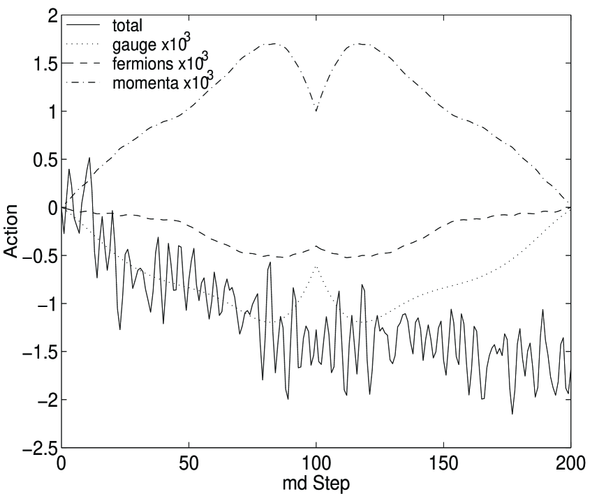
Figure 1: Action variation in a forward-backward trajectory. The initial action has been subtracted. $R<10^{-10}$ was used as a stopping criterion and $\delta t=0.010$.

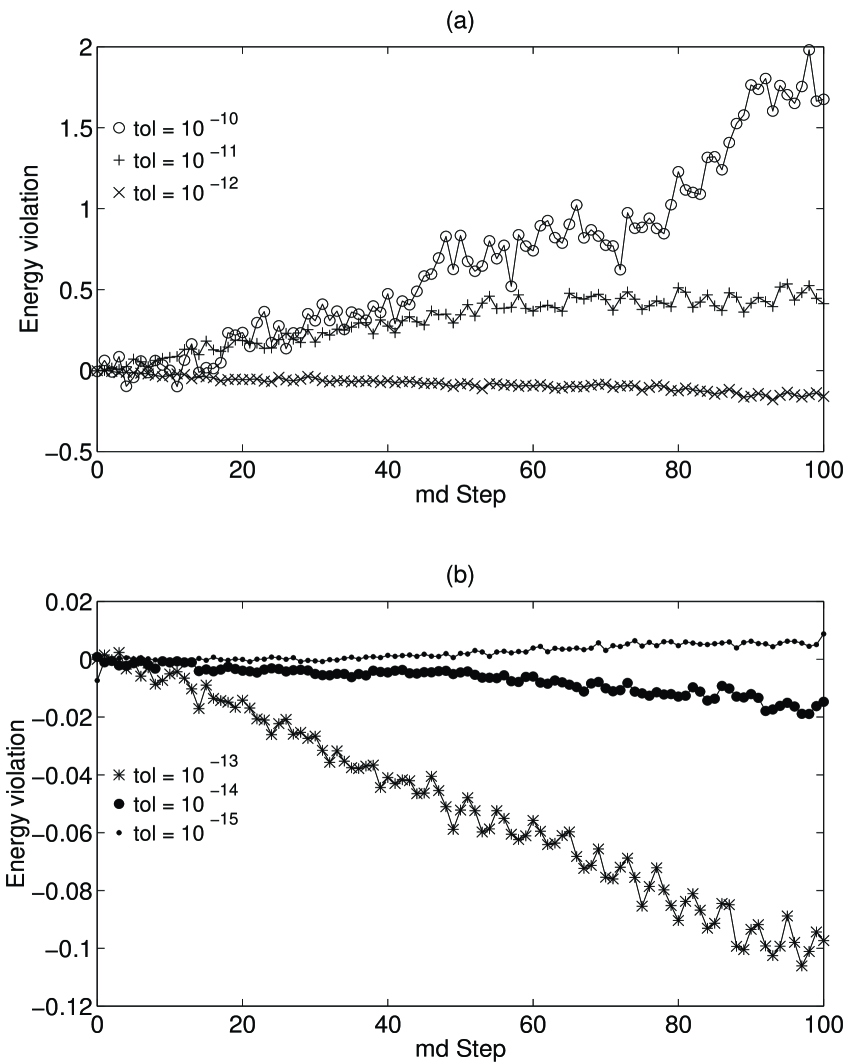
Figure 2: Reversibility violations for the energy differences in a forward-backward trajectory with the stopping conditions $R=10^{-10},10^{-11},10^{-12}$ (a) and $R=10^{-13},10^{-14},10^{-15}$ (b).

A critical issue is the requirement to converge accurately to the final solution for $\chi$. Unless you start from a value of $\chi$ which is independent of past values (e.g. $\chi=\varphi$), the initial guess introduces an element of non-reversible dynamics and therefore a failure of detailed balance. Even in one of the most commonly used HMC methods, starting from the last value of $\chi$ (or a constant extrapolation), failure to converge to the correct inverse introduces a bias that breaks time reversal invariance. In principle, only if the CG has converged exactly to the fixed point of the conjugate gradient iterations, there will be no violation of time reversal invariance. In practice, we have measured this source of error by explicitly reversing the MD dynamics for various values of the stopping conditions (see Eq. 10). In Figures 1,2 we show examples for $R=10^{-10}$, $R=10^{-11}$, $R=10^{-12}$, $R=10^{-13}$, $R=10^{-14}$ and $R=10^{-15}.$ In Figure 1 we can see the action variation (total, fermion, gauge and momenta) in a trajectory that goes forward in MD time 100 steps and then is reversed for 100 steps. We have subtracted the initial action, so if the dynamics conserves energy, the total action should remain zero and if the dynamics is reversible, the total action should be symmetric around the MD time $t=100$.

Our data demonstrates that simulations with $R\geq 10^{-12}$ are not sufficient to ensure a reversible dynamics. In Figure 2, we plot the total action difference between symmetric points in a forward-backward trajectory. If the dynamics is reversible, this difference should be zero. In this figure we can see that for $R>10^{-13}$ the dynamics is not reversible. For $R=10^{-13}$ the action difference observed is of order of $10^{-2}$ where the total action is of order $10^{7}$, which means that we are at the boundaries of single precision accuracy. However, for $R=10^{-14}$ we are well bellow the single precision accuracy. Smaller action variations can not be detected. Consequently, we chose to run our simulation using $R=10^{-14}$ as the conjugate gradient stopping criterion.

We measured the total number of CG steps needed to invert the Dirac Matrix to a given precision. The CPU time for a single leap-frog trajectory is practically proportional to the number of CG steps. However, the true performance of the method should be judged by the total number of CG steps needed to evolve the system for a fixed MD time, i.e. the total number of CG steps needed to compute a trajectory of time length $T$. We define the quantity,

$$CT={N_{CG}\over\delta t}\;,$$ (11)

which is proportional to the “computational time”. Moreover, since a smaller step size will improve the acceptance rate, the trade-off may be even more favorable for small $\delta t$, and this effect should also be included in an overall measure of efficiency. However, because we always worked with $\delta t$ in a region of very good acceptance rates ($>99\%$), we have not included this effect in our estimate of overall efficiency in our simulations.

IV. Chronological Inverter for QCD

We began our investigation by considering a trial solution, $\chi(0)$, of the new Dirac matrix $A(0)$, as a linear superposition of old solutions,

$$\chi_{trial}=c_{1}\;\chi(t_{1})+c_{2}\;\chi(t_{2})+\cdots+c_{N}\;\chi(t_{N}).$$ (12)

To simplify our notation, we will always suppose that the new inverse is computed at $t=0$, given the past values at $t_{i}$, with $\cdots<t_{3}<t_{2}<t_{1}<0$. In practice, this is usually a regular series of values $t_{n}=-n\;\delta t$ with an integration step $\delta t$.

To date HMC simulations have used either the past solution as a trial solution, $\chi_{trial}=\chi(t_{1})$, or a linear [6, 7] extrapolation, $\chi_{trial}=2\chi(t_{1})-\chi(t_{2})$. It is natural to try to improve the estimate for the trial value by using higher order polynomial extrapolations. For example, if one uses an N-th order polynomial to fit N+1 past values, the coefficients are given by

$$c_{k}~{}=~{}(-1)^{k-1}~{}{N!\over k!(N-i)!}\;.$$ (13)

Although substantial improvements can be made using higher order polynomial extrapolations, we found that the method breaks down for large N. We have also considered using over constrained fits and some estimators based on a Kalman filter. But we soon discovered that a more appealing approach to the extrapolation problem.

Since the conjugate gradient method is in fact just a minimal residual technique confined to the Krylov [11] subspace spanned by vectors $A^{j-1}\chi_{trial}$, why not start by examining a “smarter” subspace based on past success for nearby times? In this spirit, we suggest determining the coefficients $c_{n}$ by minimizing the functional,

$$\Psi[\chi]=\chi^{\dagger}M^{\dagger}M\chi-\varphi^{\dagger}\chi-\chi^{\dagger}\varphi\ ,$$ (14)

which is the same functional minimized by the Conjugated Gradient method itself. This corresponds to the minimization of the norm of the residual in the norm of the inverse matrix,

$$r^{\dagger}{1\over M^{\dagger}M}r=\chi^{\dagger}M^{\dagger}M\chi-\varphi^{\dagger}\chi-\chi^{\dagger}\varphi+b^{\dagger}b\;,$$ (15)

in the subspace spanned by $\chi_{i}\equiv\chi(t_{i})$, where $r=\phi-M^{\dagger}M\chi$ and $b\equiv(M^{\dagger})^{-1}\varphi$. Therefore we call this method “Chronological Inverter by Minimal Residual Extrapolation” or MRE. The minimization condition reduces to

$$\sum_{j=1}^{N}~{}{\chi_{i}}^{\dagger}M^{\dagger}M\chi_{j}\;c_{j}={\chi_{i}}^{\dagger}\varphi\;.$$ (16)

The only technical problem is that this system can be poorly conditioned because the past solutions $\chi_{i}$ differ from each other by order $\delta t$. However, if properly handled, this instability should not affect the resulting minima of the quadratic form in the span of the vectors, $\chi_{i}$. We have explored other methods of extrapolations to some extent, in particular other slightly different definitions of residue (not in the norm of the inverse matrix) were examined, but nothing appears at present to out-perform the Minimal Residual Extrapolation method.

V. Chronological Inverter by Minimal Residual Extrapolation

We implemented this method by calling a routine that minimizes the residual in the subspace of the past solutions, right before each CG in the usual leapfrog. This routine has as inputs the set of past vectors $\chi_{i},~{}i=1...N$ and returns a vector $\chi_{trial}$ that minimizes $\Psi[\chi]$ in the span($\chi_{i}$):

MRE Algorithm

• Construct an orthogonal basis $v_{i}$ in the span($\chi_{i}$) using the Gram-Schmidt procedure.

• Form the sub-matrix $G_{nm}={v_{n}}^{\dagger}M^{\dagger}Mv_{m}$, and the vector $b_{n}={v_{n}}^{\dagger}\varphi$.

• Solve $G_{nm}a_{m}=b_{n}$ using the Gauss-Jordan method.

• Return the trial vector $\chi_{trial}=\sum_{n=1}^{N}~{}a_{n}v_{n}$.

Because $\chi_{i}$’s are nearly linearly dependent there is a numerical instability, and the Gram-Schmidt procedure does not produce a true basis of span($\chi_{i}$) due to round off error. Hoverer span($v_{i}$) is a subspace close enough to the relevant subspace of the old solutions. Because the accumulated error is larger at the late stages of the Gram-Schmitt iteration, the ordering of the $\chi_{i}$ is important. We get better results if we number the $\chi_{i}$’s from the newest to the oldest. This way we quite accurately pick up the new relevant directions, while the old ones, which are less relevant, are computed with more round off error. In this way we can handle the numeric instability and turn it to our advantage.

This method requires $(N^{2}+5N)/2$ dot products and $N$ $M\chi$ matrix-vector applications, and the storage of $3N$ past pseudo-fermion configurations. There are other implementations of the above concepts which can do the same thing using less memory. But most of them suffer from numerical instabilities. The best we found, and actually used in our production runs, is instead of storing $\chi^{\prime}s$, store $v^{\prime}s$, keeping them in the right order - most recent first. This reduces the memory requirement to the storage of $2N$ pseudo-fermion configurations, and has the same performance as the original method. We checked this method using double precision, and there was no visible improvement by reducing the round off-error.

In Table 1, we record the mean number of CG steps required to reach the solution normalized relative to starting with $\chi_{trial}=\varphi$. We used the stopping condition that the normalized squared residual (10) was smaller than $10^{-14}$.

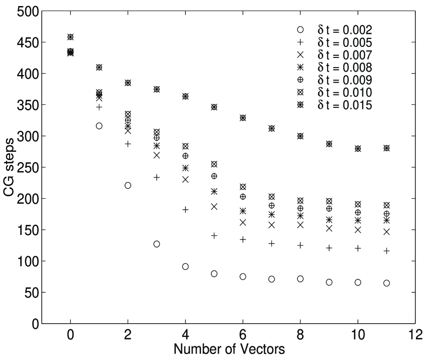
Figure 3: Number of CG steps vs. number of vectors for various values of $\delta t$ for the Minimal Residual Extrapolation method.

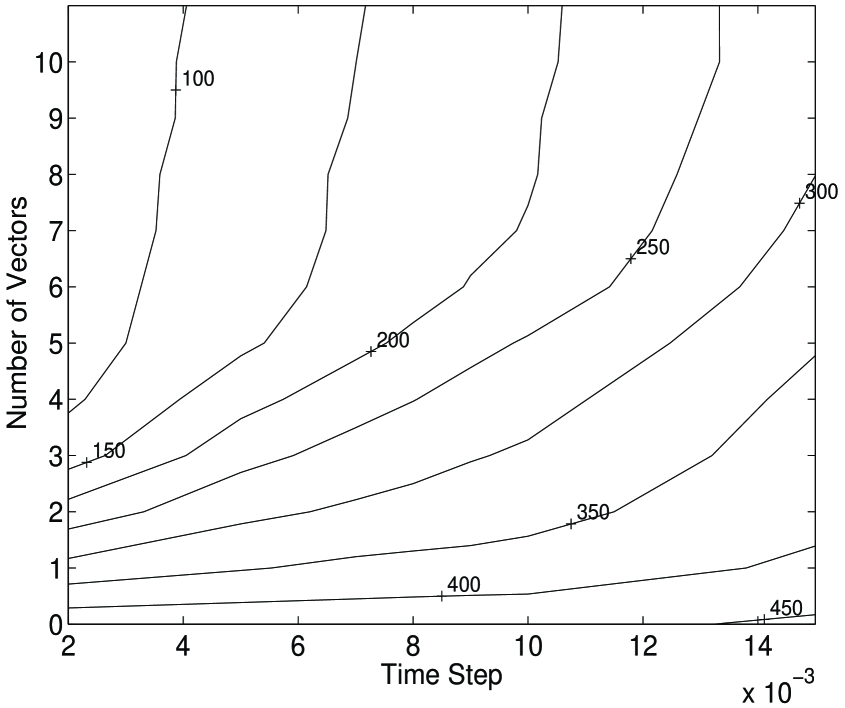
Figure 5: Contour plot of number of CG steps.

The data (see Table 1 and Figures 3,  4 ), suggest that the more vectors you keep from the past the better starting residue you achieve, and as a result the fewer CG steps you need in order to converge to a given accuracy. Furthermore the number of CG steps is decreasing as $\delta t$ is decreasing. We have also presented our results as a contour plot in Figure 5 for the number of iterations as a function of the number of vectors versus the time step.

N=0	1.00	1.00	1.00	1.00	1.00	1.00	1.00
N=1	0.73	0.80	0.84	0.85	0.85	0.86	0.90
N=2	0.52	0.67	0.72	0.73	0.76	0.78	0.84
N=3	0.30	0.55	0.63	0.67	0.70	0.72	0.82
N=4	0.21	0.44	0.55	0.59	0.63	0.67	0.79
N=5	0.18	0.33	0.45	0.51	0.56	0.61	0.76
N=6	0.18	0.32	0.38	0.43	0.49	0.53	0.72
N=7	0.17	0.30	0.38	0.42	0.45	0.48	0.68
N=8	0.17	0.30	0.37	0.41	0.42	0.47	0.66
N=9	0.15	0.28	0.36	0.39	0.44	0.47	0.63
N=10	0.15	0.29	0.36	0.39	0.42	0.45	0.61
N=11	0.15	0.27	0.35	0.39	0.42	0.45	0.62
$\delta t$	0.002	0.005	0.007	0.008	0.009	0.010	0.015

Table 1: Number of CG steps needed to converge to the solution from minimum residual extrapolation. The table is normalized with respect to N = 0 (i.e. no extrapolation, $\chi_{trial}=\varphi$). The statistical errors are of the order of 10%.

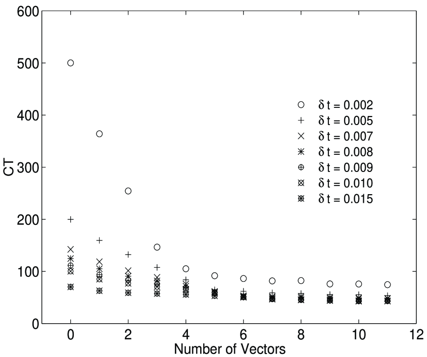
Figure 6: CT vs. number of vectors for various values of $\delta t$ for the Minimal Residual Extrapolation method.

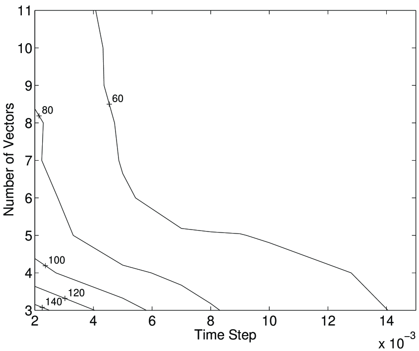
Figure 7: Contour plot of CT for the Minimal Residual Extrapolation method.

As explained above, the performance of the method given in “computational time” CT is summarized in Table 2, and in Figures 6,7. It is interesting to note how CT depends on the number of the vectors retained. Unlike the number of CG steps, CT does not decrease as $\delta t$ becomes smaller. Moreover, one can see from Figure 7 that there is a range of $\delta t$ where the performance is relatively insensitive to $\delta t$. As you decrease the step size, you gained back almost the same performance by reducing proportionally the number of CG steps required for convergence in each step. As discussed earlier, smaller step sizes have the extra advantage of improving the acceptance rate.

N=0	5.86	2.34	1.66	1.46	1.30	1.17	0.78
N=1	4.29	1.88	1.40	1.24	1.10	1.00	0.70
N=2	3.03	1.57	1.20	1.07	0.98	0.91	0.66
N=3	1.78	1.29	1.06	0.96	0.91	0.84	0.64
N=4	1.23	1.02	0.92	0.86	0.82	0.78	0.62
N=5	1.08	0.78	0.74	0.74	0.73	0.71	0.59
N=6	1.04	0.74	0.64	0.63	0.63	0.62	0.56
N=7	0.99	0.71	0.63	0.61	0.58	0.57	0.53
N=8	0.98	0.69	0.62	0.60	0.57	0.55	0.51
N=9	0.88	0.67	0.60	0.58	0.57	0.54	0.49
N=10	0.90	0.67	0.60	0.57	0.55	0.53	0.48
N=11	0.88	0.64	0.59	0.57	0.54	0.53	0.48
$\delta t$	0.002	0.005	0.007	0.008	0.009	0.010	0.015

Table 2: Computational Time (CT) starting from minimum residual extrapolation. The table is normalized to 1 at $\delta t=0.010$ for N = 1 ( $\chi_{trial}=\chi_{last}$).

VI. Comparison with the Polynomial Extrapolation Method

The polynomial extrapolation method has the advantage that it requires very little computational effort, just a local sum on each lattice point with fixed coefficients given once and for all by equation (13), costing less than a single CG step. For a polynomial of order $N$, the only storage requirement is for the previous $N$ pseudo-fermion configurations, $\chi(t_{i})$.

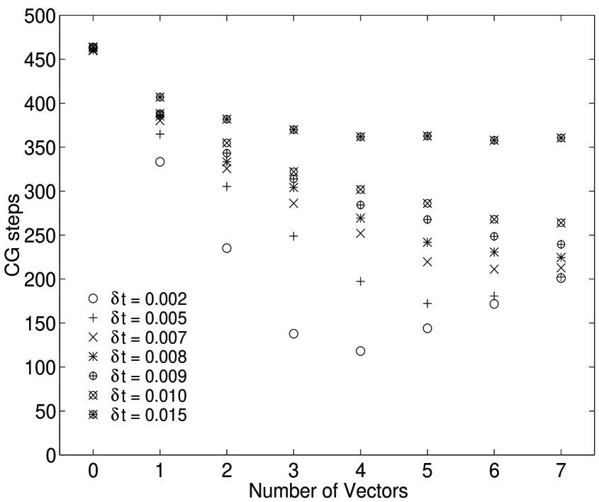
Figure 8: Number of CG steps vs. number of vectors for various values of $\delta t$ for the Polynomial extrapolation.

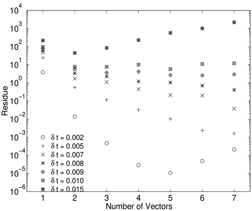
Figure 9: Starting residue vs. number of vectors for various values of $\delta t$ for the polynomial extrapolation.

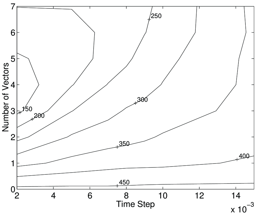
Figure 10: Contour plot of number of CG steps for the Polynomial extrapolation.

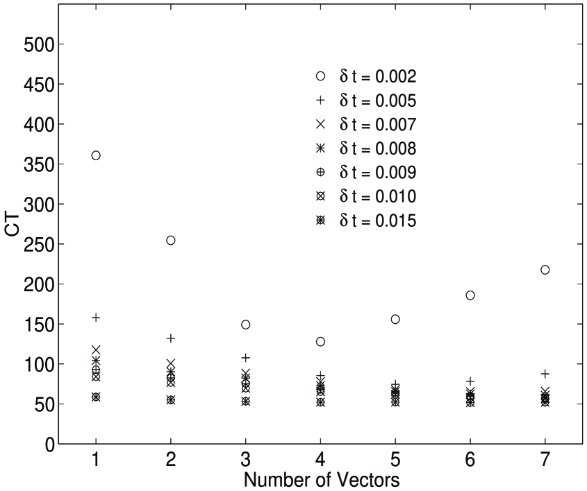
Figure 11: CT vs. Number of vectors for various values of $\delta t$ for the Polynomial extrapolation.

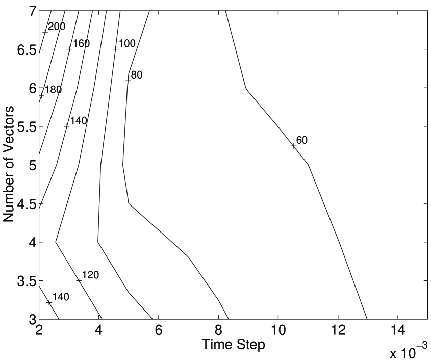
Figure 12: Contour plot of CT for the Polynomial extrapolation.

Results of the polynomial extrapolation are shown in Tables 3,4 and Figures 8,9,10,11, 12. Again, to compare efficiencies, the CG iterations should be divided by $\delta t$, so we compare the total number of CG steps needed to evolve the system for a fixed distance in configuration space. Note that if $\delta t$ is large, the overall performance is good, but the acceptance will drop drastically. If $\delta t$ is small, the extrapolation is excellent, but the system will evolve too slowly in phase space. It is noteworthy that we find a window in $\delta t$ where both the acceptance is good and the extrapolation works well.

N=0	1.00	1.00	1.00	1.00	1.00	1.00	1.00
N=1	0.72	0.79	0.82	0.83	0.84	0.84	0.88
N=2	0.51	0.66	0.70	0.72	0.74	0.77	0.83
N=3	0.30	0.54	0.62	0.66	0.68	0.70	0.80
N=4	0.26	0.43	0.55	0.58	0.62	0.65	0.78
N=5	0.31	0.37	0.48	0.52	0.58	0.62	0.79
N=6	0.37	0.39	0.46	0.50	0.54	0.58	0.77
N=7	0.44	0.44	0.46	0.49	0.52	0.57	0.78
$\delta t$	0.002	0.005	0.007	0.008	0.009	0.010	0.015

Table 3: Number of CG steps to reach the solution for polynomial extrapolation. Normalized to 1 for N = 0 ($\chi_{trial}=\varphi$).

N=0	5.96	2.38	1.69	1.48	1.32	1.20	0.79
N=1	4.29	1.88	1.40	1.24	1.11	1.00	0.70
N=2	3.03	1.57	1.20	1.07	0.98	0.91	0.66
N=3	1.78	1.28	1.05	0.98	0.90	0.83	0.64
N=4	1.52	1.01	0.93	0.87	0.81	0.78	0.62
N=5	1.85	0.89	0.81	0.78	0.77	0.74	0.62
N=6	2.21	0.93	0.78	0.74	0.71	0.69	0.61
N=7	2.59	1.04	0.78	0.72	0.69	0.68	0.62
$\delta t$	0.002	0.005	0.007	0.008	0.009	0.010	0.015

Table 4: Computational Time (CT) starting from polynomial extrapolation. The table is normalized to 1 at $\delta t=0.010$ for N = 1 ($\chi_{trial}=\chi_{last}$).

We also note that the coefficients of the Minimal Residual Extrapolation method (12), which á priori are generic complex numbers, are in fact very close to coefficients in the polynomial extrapolation (13) for the first few orders. One way to understand this coincidence is to observe that for a smooth evolution the determination of coefficients $c_{i}$,

$$\chi_{trial}=c_{1}\;\chi(t_{1})+c_{2}\;\chi(t_{2})+\cdots+c_{N}\;\chi(t_{N}),$$ (17)

by a polynomial fit is equivalent to fixing the coefficients by making a Taylor expansion of each term, $\chi(t_{n})$, in $t_{n}=n\delta t$ canceling all contributions to $O(\delta t^{N})$. To prove this we solve the constraints

$$\sum_{n=1}^{N}(t_{i})^{n-1}\;y_{n}=\chi(t_{i})\;,$$ (18)

for a polynomial fit $y(t)~{}=~{}y_{1}+t\;y_{2}+\cdots+\;t^{N-1}\;y_{N}$ to find $y_{1}=\chi_{trial}$. Then show that $y_{1}=\sum_{i}c_{i}\chi(t_{i})$ when we enforce the Taylor series constraints,

$$\sum_{i=1}^{N}(t_{i})^{n-1}\;c_{i}=\delta_{1,n}\ .$$ (19)

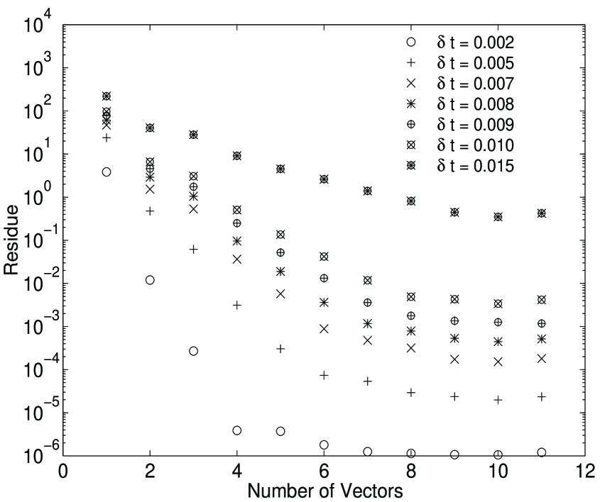
Figure 4: Starting residue vs. number of vectors for various values of $\delta t$ for the Minimal Residual Extrapolation method.

From this exercise, we conclude that the success of the polynomial fit probably results from the local convergence of the power series MD in time. On the other hand, if we compare the magnitude of the estimated residual of the Minimal Residual Extrapolation (MRE) versus the Polynomial Extrapolation (see Figures 4, 9), we notice that while the polynomial actually deteriorates at high order, the minimal residual continues to improve. In our simulation for a polynomial extrapolation of order of $N=5-6$, the deterioration becomes appreciable.

In conclusion the increased efficiency of the MRE method is worth the extra computational effort (equivalent to $N/2$ CG steps). With a Polynomial Extrapolation, one gets poor results on a few exceptional lattices, whereas the MRE method is a more robust estimator, which implements a kind of self-tuned extrapolation, never doing worse than a polynomial fit of the same order.

VII. Projective Conjugate Gradient

It is natural at this point to try to understand why the Chronological Inverter is working and to explore more effective methods of using the past information. We have performed a large number of “numerical experiments” to gain some understanding. In particular we have shown that if one assumes complete knowledge of the inverse of the matrix in the immediate past $A_{1}\equiv A(t_{1})$ and performs a perturbation expansion in the difference $V=A-A_{1}$ convergence is poor unless $\delta t$ is very small on the order of $10^{-3}$. On the other hand, although we know no way to efficiently implement the idea, if we use $A_{1}$ as a preconditioner for the conjugate gradient iterations of A, a spectacular acceleration of the conjugate gradient is achieved — for $\delta t=0.01$ converging to $R=10^{-16}$ in about 15 iterations. In this way, we are now convinced that the use of past information as a preconditioner holds out even greater promise. We are engaged in on going research in this regard. However, here we report a minor extension of the current method along these lines.

In the Minimal Residual Extrapolation, we suggest re-using our past solutions $\{\chi_{i}\}$ to construct a preconditioner for the subsequent CG iterations. The straight forward modification is as follows. Since we have already minimized the functional $\Psi(\chi)$ in the subspace spanned by $\chi_{i}$’s, it is reasonable to require that all the subsequent search directions we generate in CG are also $A$-conjugate to this subspace. This will ensure that at any step $K$ of CG, we obtain the global minimum of $\Psi(\chi)$ in the space spanned by $\chi_{i}$’s and $p_{k}$ ($k=1..K$). This requirement is implemented by almost the same technique used in conventional preconditioners for CG [11]. In each CG iteration, the residual $r_{k}$ is replaced by an improved search direction vector $z_{k}$. Thus we propose for our Projected Conjugate Gradient (PCG) method that the vector $z$ is chosen to be the A orthogonal component of $r$ with respect to span($\chi_{i}$) or in terms of the basis vectors basis $v_{n}$ defined above for our MRE algorithm (see Section V)

$$z=r-\lambda_{n}v_{n},$$ (20)

where the condition $v^{\dagger}_{n}Az=0$ means

$$G_{nm}\lambda_{m}=v^{\dagger}_{n}M^{\dagger}Mr$$ (21)

with $A=M^{\dagger}M$ and $G_{nm}={v_{n}}^{\dagger}M^{\dagger}Mv_{m}$ defined as before. The coefficients $\lambda_{n}$ are found by solving a small linear system using the Gauss-Jordan elimination method or the LU factorization. The amount of computation for solving such a system is very small, especially if one uses the LU factorization, since the matrix $G_{nm}$ is computed once and the LU factors can be used in subsequent steps. As a result we modify the conjugate gradient routine as follows:

PCG Algorithm

• Project residue: $z_{k}=r_{k}-v_{n}(G^{-1})_{n,m}(v^{\dagger}_{m}M^{\dagger}Mr_{k})$

• Compute search direction: $p_{k}=z_{k-1}-\beta_{k-1}p_{k-1}$, where $\beta_{k-1}=r_{k-1}^{\dagger}z_{k-1}/r_{k-2}^{\dagger}z_{k-2}$.

• Compute new solution: $\chi_{k}=\chi_{k-1}+\alpha_{k}p_{k}$, where $\alpha_{k}=r_{k-1}^{\dagger}z_{k-1}/p_{k}^{\dagger}M^{\dagger}Mp_{k}$

• Compute new residual: $r_{k}=r_{k-1}-M^{\dagger}Mp_{k}$.

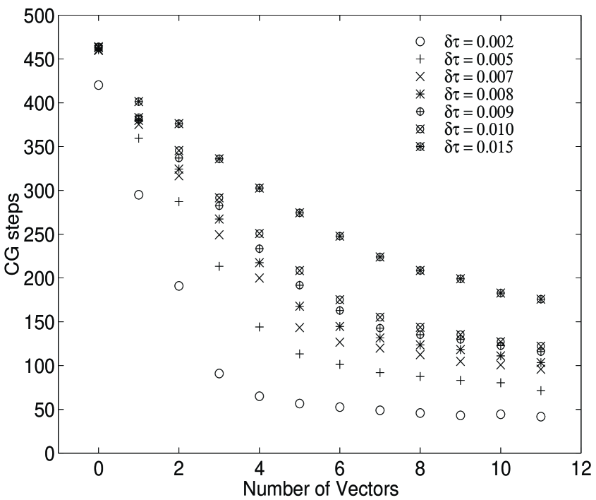
Figure 13: Number of CG steps vs. number of vectors for various values of $\delta t$ for the Projective CG.

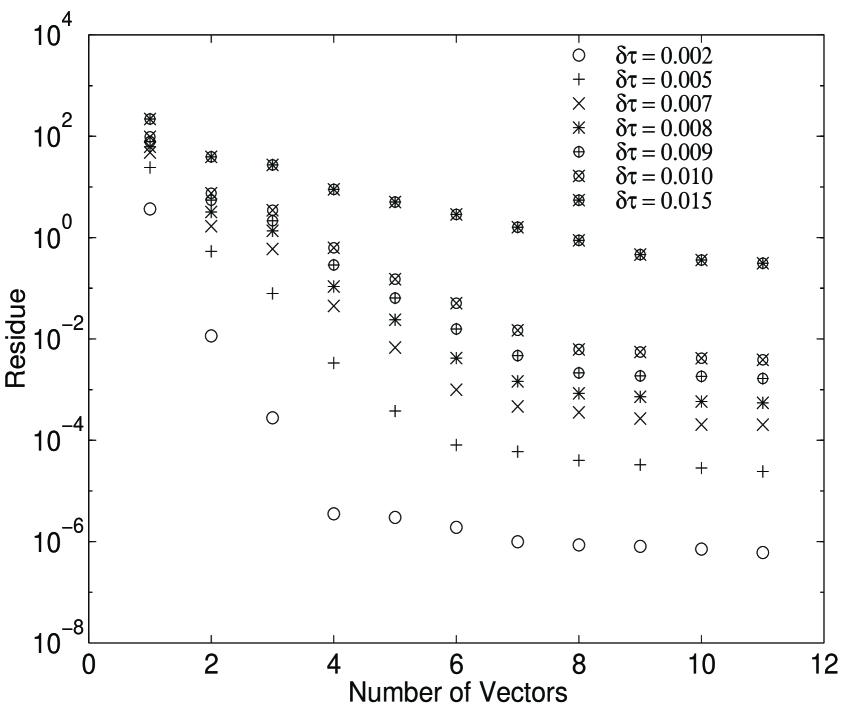
Figure 14: Starting residue vs. number of vectors for various values of $\delta t$ for the Projective CG.

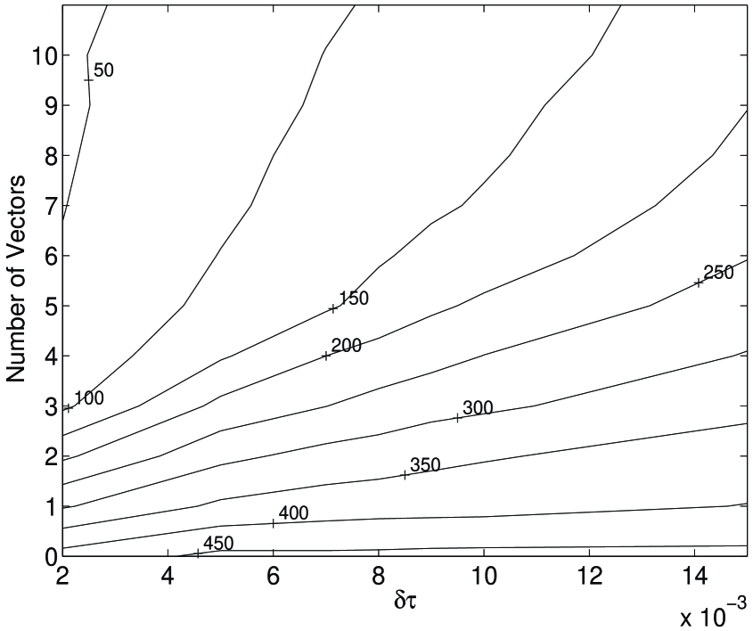
Figure 15: Contour plot of number of CG steps for the Projective CG.

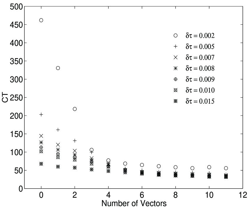
Figure 16: CT vs. Number of vectors for various values of $\delta t$ for the Projective CG.

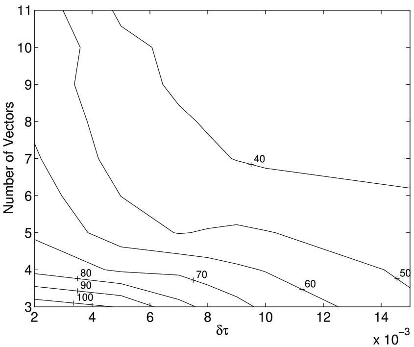
Figure 17: Contour plot of CT for the Projective CG.

It can easily be shown that the above algorithm produces a set of search vectors that are A-conjugate among themselves and to the $v_{i}$’s. The only time consuming step, needed every CG iteration, is the computation of the right-hand side ${v_{n}}^{\dagger}M^{\dagger}Mr_{k}$, but the vectors $\tilde{v}_{n}=M^{\dagger}Mv_{n}$ have in fact already been computed in the MRE step so this only involves N scalar products. For our implementation on the MIT 128-node CM-5, one $M^{\dagger}M\chi$ operation is equivalent to 55 ${\tilde{v}}^{\dagger}r$ operations so with O(10) vectors the overhead is about 20%. This cost has been taken into account when analyzing the performance of this algorithm. The results of our performance tests are summarized in Tables 5,6 and in Figures 13,14,15,16,17.

N=0	1.00	1.00	1.00	1.00	1.00	1.00	1.00
N=1	0.65	0.79	0.82	0.84	0.84	0.84	0.88
N=2	0.42	0.63	0.70	0.71	0.74	0.76	0.83
N=3	0.20	0.47	0.55	0.59	0.62	0.64	0.74
N=4	0.14	0.32	0.44	0.48	0.51	0.55	0.67
N=5	0.12	0.25	0.32	0.37	0.42	0.46	0.60
N=6	0.12	0.22	0.28	0.32	0.36	0.39	0.54
N=7	0.11	0.20	0.26	0.29	0.31	0.34	0.49
N=8	0.10	0.19	0.25	0.27	0.30	0.32	0.46
N=9	0.09	0.18	0.23	0.26	0.29	0.30	0.44
N=10	0.09	0.18	0.22	0.24	0.27	0.28	0.40
N=11	0.09	0.16	0.21	0.23	0.25	0.27	0.39
$\delta t$	0.002	0.005	0.007	0.008	0.009	0.010	0.015

Table 5: Number of the projective CG steps needed to converge to the solution. We used Minimal Residual Extrapolation to obtain the initial trial solution $\chi$. The table is normalized with respect to N = 0 (i.e. no extrapolation, $\chi_{trial}=\varphi$). The statistical errors are of the order of 10%.

N=0	5.38	2.36	1.68	1.47	1.32	1.18	0.79
N=1	3.85	1.88	1.40	1.24	1.11	1.00	0.70
N=2	2.54	1.53	1.20	1.08	1.00	0.92	0.67
N=3	1.23	1.16	0.97	0.91	0.85	0.79	0.61
N=4	0.90	0.80	0.79	0.75	0.72	0.69	0.55
N=5	0.80	0.64	0.58	0.59	0.60	0.59	0.51
N=6	0.75	0.58	0.52	0.52	0.52	0.50	0.47
N=7	0.71	0.54	0.50	0.48	0.46	0.45	0.44
N=8	0.68	0.52	0.48	0.46	0.45	0.43	0.41
N=9	0.65	0.50	0.45	0.45	0.44	0.41	0.40
N=10	0.68	0.49	0.44	0.43	0.42	0.39	0.37
N=11	0.65	0.44	0.43	0.40	0.40	0.38	0.37
$\delta t$	0.002	0.005	0.007	0.008	0.009	0.010	0.015

Table 6: Computational Time (CT) for the minimum residual - projective CG algorithm. The table is normalized to 1 at $\delta t=0.010$ for N = 1 ( $\chi_{trial}=\chi_{last}$).

Our simulations show that the Minimal Residual Extrapolation algorithm followed by the PCG algorithm gives us an extra $30\%$ improvement over the Minimal Residual Extrapolation followed by the standard CG. In general the actual improvement of the performance depends crucially on the dot product versus Matrix-Vector product speed that a given computer can achieve.

VIII. Conclusions

Let us summarize our perspective on the problem of accelerating a time sequence of conjugate gradient inverters. The chronological method has offered significant performance improvement, but at the same time the results are tantalizing. Just by starting from the old solution, the residue is reduced by 4 orders of magnitude to order $10^{-4}$, relative to the residue with $\chi=\varphi$. Then if we look at Figure 18, we see that the residue is reduce further by 5 orders of magnitude using 10 additional past solution vectors in our Minimal Residual Extrapolation method. Finally, the first 10 CG iterations accounts for another 2 orders of magnitude. However accurate reversibility ultimately requires us to reduce the residue by another 4 more orders. This last 4 orders of magnitude takes several hundred additional vectors in the CG iterations. We are both intrigued and frustrated by the observation that we can reduce the residue by 11 orders of magnitude in a 20-30 dimensional vector space, but then the standard CG iterations requires hundreds of additional search directions to accomplish the remaining 4 orders of magnitude needed to satisfy adequately the reversibility constraint. It is tempting to hope that further improvements can be made on this last 4 orders of magnitude.

We have emphasized the analytic properties of $\chi(t)$ because we believe it may suggest ways to understand and further improve the chronological method. For example, the failure at fixed $\delta t$ to improve the polynomial extrapolation by increasing indefinitely the number of terms is probably a signal of nearby singularities. Our success so far is probably due to the slow evolution of the low eigenvalues of the Dirac operator. Thus we are in essence taking advantage of “critical slowing down” in the HMC algorithm to accelerate the Dirac inverter. However, there may well be other vectors (besides the final solution) in the nearby past iteration that can better exploit the slow evolution of our matrix. For example, the last CG routine, which is closest in time to our present inverter, itself generates many A conjugate search vectors, that may be more useful than the older solutions exploited in our MRE method. In addition this subspace of past vectors might be used not just as a way to arrive at an initial guess, but also as a way to accelerate (or “precondition”) the iterative process itself. In this spirit the Projective CG method presented in section VII was included to illustrate how in principle a set of past vectors can be exploited to accelerate the convergence of the CG algorithm itself. We are currently studying such chronological preconditioners more systematically.

In conclusion, we found that the procedures presented here, and in particular the Minimal Residual Extrapolation method reduces by a factor of about 2-3 the mean number of conjugate gradient iterations required to move in phase space for a fix molecular dynamics time. This is achieved with negligible extra computational time, at the expense of memory. Consequently when sufficient memory is available for storing the past solutions the Dirac inverter, our Chronological Inversion method certainly provides one more useful trick for more efficiently generating full QCD configurations.

Acknowledgments: We would like to thank D. Castanon, C. Evangelinos and C. Rebbi for many helpful discussions. This work was supported in part by funds provided by the U. S. Department of Energy under grand DE–FG02–91ER400688, Task A, and under cooperative agreement #DF-FC02-94ER40818.

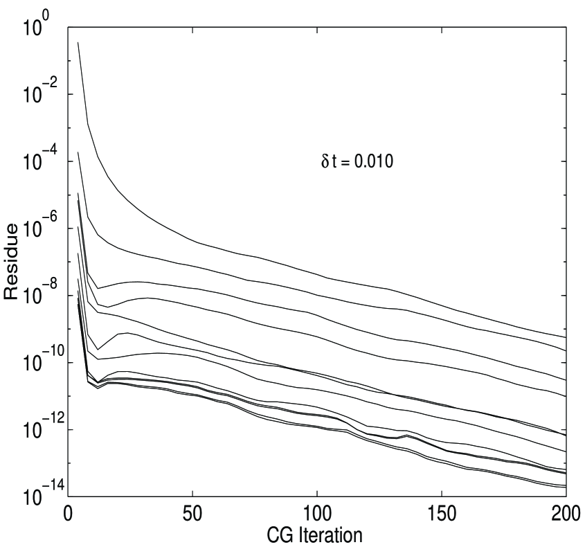
Figure 18: Example of convergence of the CG as a function of the number of extrapolation vectors for a single lattice and $\delta t=0.010$. The method used was Minimal Residual Extrapolation and the number of vectors varies from $0$ (top line) to $11$ (bottom line).

References

- [1] R.D. Mawhinney, The status of the Teraflops projects, Nucl.Phys. (Proc. Supl) B42 (1995) 140.
- [2] G. Parisi and Y. Wu, Sci. Sin. 24, (1981) 483; J. Polonyi and H.W. Wyld, Phys. Rev. Lett. 51, (1983) 2257; S. Duane, Nucl. Phys. B257, (1985) 652; G.C. Batroumi, G.R. Katz, A.S. Kronfeld, G.P. Lapage, B. Svetisky, and K.G. Wilson, Phys. Rev. D 32, (1985) 2736. S. Duane and J. Kogut, Phys. Rev. Lett. 55, (1985) 2774, Nucl. Phys. B275, (1986) 398; J. Callaway and A. Rhaman, Phys. Rev. D34, (1986) 7911; S. Duane, A.D. Kennedy, B.J. Pendleton and D. Roweth, Phys. Lett B195 (1987) 216; S. Gottlieb, W. Liu, D. Toussaint, R.L. Renken and R.L. Sugar, Phys Rev. D 35 (1987) 2531; R. Gupta, G.W. Kilcup and S.R. Sharpe, Phys. Rev. D38, (1988) 1278; R. Gupta et al., Phys. Rev. D40 2072 (1989), and D44 (1991) 3272.
- [3] “Those who cannot remember the past are condemned to repeat it.”, George Santayana, The Life of Reason or Phases of Human Progress, New York, 1917.
- [4] R.C. Brower, A.R. Levi and K. Orginos, “Extrapolation Methods for the Dirac Inverter in Hybrid Monte Carlo”, talk presented at Lattice 94, Nucl. Phys. (Proc. Supl) B42 (1995) 855.
- [5] M. Lüscher Nucl. Phys. B418 (1994) 637.
- [6] S. Gottlieb, W. Liu, D. Toussaint, R.L. Renken and R.L. Sugar, Phys Rev. D35 (1987) 2531.
- [7] R. Gupta, G. Kilcup, S. Sharpe, Phys Rev. D38 (1988) 1278; R. Gupta, A. Patel, C. Baile, G. Guralnik, G. Kilcup, S. Sharpe, Phys Rev. D40 (1989) 2072; R. Gupta, C. Baile, R Brickner, G. Kilcup, A. Patel, S. Sharpe, Phys Rev. D44 (1991) 3272.
- [8] A.H. Jazwinski,”Stochastic Processes and filtering Theory”, NY Academic Press (1970).
- [9] C. Hill and J. Marshall,”Applications of parallel Navier Stokes solvers to Ocean Modelling.” Proc. of Parallel CDF 95 (Caltech) (1995).
- [10] T. DeGrand, and P. Rossi, Comp. Phys. Comm. 60 (1990) 211.
- [11] G. Golub, C. Van Loan. Matrix Computations, second edition, (The John Hopkins University Press, Baltimore, 1990)