Critical Behaviour of the Two Dimensional
Step Model
A.C. Irving and R. Kenna
DAMTP, University of Liverpool L69 3BX, England

August 1995

We use finite–size scaling of Lee–Yang partition function zeroes to study the critical behaviour of the two dimensional step or sgn $O(2)$ model. We present evidence that, like the closely related $XY$–model, this has a phase transition from a disordered high temperature phase to a low temperature massless phase where the model remains critical. The critical parameters (including logarithmic corrections) are compatible with those of the $XY$–model indicating that both models belong to the same universality class.

1 Introduction

In a recent paper [1], we demonstrated the power of finite–size scaling applied to Lee–Yang zeroes [2] in uncovering logarithmic corrections to scaling in the two–dimensional $XY$– or $O(2)$ spin model. In this paper we apply the same techniques to the closely related ‘step model’ [3, 4], also known [5, 6] as the sgn $O(2)$ model. The question of criticality of this model has, until now, been unresolved despite several analyses based on high temperature series (see [6] for a review) and on numerical simulation [7, 8]. The interest in the model arises from its possible membership of the $XY$–model universality class which exhibits the Kosterlitz–Thouless [KT] phase transition [9]. Like the $XY$–model, the step model has a configuration space which is globally and continuously symmetric. Unlike the $XY$–model, however, the interaction function is discontinuous and the Mermin–Wagner theorem [10] does not apply. Nonetheless, it is expected that if a phase transition exists in the step model, it should not be to a phase with long range order [4, 8, 11].

Sánchez–Velasco and Wills [8] presented evidence of critical behaviour starting at $\beta_{c}=1/T_{c}=0.91\pm 0.04$. This was based on finite–size scaling [FSS] of the spin susceptibility. Since the associated critical index $\eta(T_{c})$ was significantly greater than that measured for the $XY$–model, it was concluded that the step and $XY$ models are not in the same universality class. In this paper we present evidence that the step model is not critical at that temperature. However it is critical at lower temperatures with a critical index $\eta(T_{c})$ compatible with the $XY$ value. The accuracy afforded by the Lee–Yang zeroes study is a crucial part of the analysis.

2 The step model and the $XY$–model

Consider the partition function

$$Z(\beta,h)=\sum_{\{{\vec{s}}_{x}\}}{e^{-\beta H+h{\hat{n}}\cdot{\vec{M}}}}\,,$$ (1)

where the Boltzmann factor is $\beta=1/kT$, ${\hat{n}}$ is a unit vector defining the direction of the external magnetic field and $h$ is a scalar parameter representing its strength. The summation is over all configurations open to the system and ${\vec{s}}_{x}$ is a unit length two-component spin at each site $x$ in the cubic lattice $\Lambda\equiv L^{d}$ ($d=2$). The magnetisation for a given configuration is

$${\vec{M}}=\sum_{x\in\Lambda}{\vec{s}}_{x}\,.$$

In the case of the $XY$–model, the interaction hamiltonian is

$$H_{{XY}}=-\sum_{x\in\Lambda}\sum_{\mu=1}^{d}{\vec{s}}_{x}\cdot{\vec{s}}_{x+\mu}\,,$$

while for the step model it is

$$H_{\rm{step}}=-\sum_{x\in\Lambda}\sum_{\mu=1}^{d}\hbox{sgn}({\vec{s}}_{x}\cdot{\vec{s}}_{x+\mu})\,.$$

Thus the continuous (cosine) dependence of the interaction energy in the usual $XY$–model is replaced by a discrete step function dependence.

The leading infinite volume critical behaviour of the 2D $XY$–model is characterized by exponential divergences (essential singularities) in the thermodynamic functions [9]. In terms of the reduced temperature $t\equiv 1-\beta/\beta_{c}\rightarrow 0^{+}$ the (leading) infinite volume scaling behaviour of the correlation length and the zero-field magnetic susceptibility is (respectively) [9]

$$\xi_{\infty}(t) \sim e^{at^{-\nu}}\,,$$ (2)

$$\chi_{\infty}(t) \sim \xi_{\infty}^{2-\eta}\,,$$ (3)

where $\nu=1/2$ and $\eta=1/4$. The $XY$–model remains critical for all $\beta>\beta_{c}$.

For models obeying the Lee–Yang theorem [2], the partition function zeroes in the magnetic field strength ($h$) plane (the Lee–Yang zeroes) are all on the imaginary axis. In the high temperature phase these zeroes remain away from the real axis, pinching it only as $t\rightarrow 0^{+}$ (in the thermodynamic limit). The zero closest to the real axis marks the edge of the distribution of zeroes and is known as the Yang–Lee edge, $z_{\rm{YL}}$. The theorem has been proved only for certain models, the $XY$–model included [12]. In [1] we used this fact to show the above leading critical behaviour for the $XY$–model and the corresponding behaviour of the Yang–Lee edge, $z_{\rm{YL}}$ are, in fact, modified by logarithmic corrections:

$$\chi_{\infty}(t) \sim \xi_{\infty}^{2-\eta}t^{r}\,,$$ (4)

$$z_{\rm{YL}}(t) \sim \xi_{\infty}^{\lambda}t^{p}\,,$$ (5)

where

$$\lambda=-\frac{1}{2}(d+2-\eta)=-{{15}\over 8}$$ (6)

and the parameters $r$ and $p$ ($=-r/2)$ are logarithmic correction indices [1]. The corresponding FSS behaviour for the susceptibility and the first zero $z_{1}$ ($=z_{YL}$) at $t=0$ is [1]

$$\chi_{L}(0) \sim L^{2-\eta}(\ln{L})^{-\frac{r}{\nu}}\,,$$ (7)

$$z_{1}(0) \sim L^{\lambda}(\ln{L})^{r}\,.$$ (8)

For the 2D $XY$–model the numerical value of $r$ was found to be small but non-zero ($-0.023\pm 0.010$) [1].

The objects of the present analaysis were to establish

1. if the scaling behaviour of the very precisely determined Yang–Lee edge would unequivocably determine whether the step model had a critical phase

2. if so, whether the phase transition is in the same universality class as the $XY$–model.

3 Method and results

The methods used are those described in [1]. A single cluster algorithm [13] is used to generate a large number of measurements (100K for each lattice size $L$ and temperature $1/\beta$) of the energy $H$ and the magnetisation ${\vec{M}}$ at zero external magnetic field. Such data were obtained for lattice sizes $L=32$, $48$, $64$, $128$ and $256$ covering the $\beta$ range $0.86$ to $1.40$ with varying degrees of spacing. Multi–histogram techniques [14, 15] were used to combine data at different values of $\beta$ and so obtain detailed $\beta$ dependence. In the neighborhood of possible critical points we used sufficiently fine spacing (typically 0.025) to ensure adequate overlap between histograms for a given size of lattice.

The partition function for a complex magnetic field ($h=h_{r}+ih_{i}$, $h_{r},h_{i}\in\mbox{\math R}$) can be written in terms of a real and an imaginary part [1, 16, 17] as

$$Z(\beta,h_{r}+ih_{i})={\rm{Re}}Z(\beta,h_{r}+ih_{i})+i{\rm{Im}}Z(\beta,h_{r}+ih_{i})\,,$$ (9)

where

$${\rm{Re}}Z(\beta,h_{r}+ih_{i}) = Z(\beta,h_{r})\langle\cos{(h_{i}M)}\rangle_{\beta,h_{r}}\,,$$ (10)

$${\rm{Im}}Z(\beta,h_{r}+ih_{i}) = Z(\beta,h_{r})\langle\sin{(h_{i}M)}\rangle_{\beta,h_{r}}\,.$$ (11)

Here the subscripts indicate that the expectation values are taken at (inverse) temperature $\beta$ and in a (real) external field $h_{r}$.

No specific proof of the Lee–Yang theorem exists for the step model. We can, however, use (10) and (11) to (numerically) determine the loci along which the real and imaginary parts of the partition function separately vanish. These formulae concern expectation values of real quantities in a real external field and at no stage is a simulation involving a complex action involved. The Lee–Yang zeroes are then the points in the complex $h$–plane where the loci intersect [17]. We have determined these loci and thereby the Lee–Yang zeroes close to the real $h$–axis. We were able to determine the first 15 zeroes and found that they lie on the imaginary $h$–axis for all the lattices studied. Thus we have numerical evidence that the step model obeys the Lee–Yang theorem. The following analysis applies to the first zeroes only (the Yang–Lee edge) and we defer the study of higher zeroes to a later paper [18].

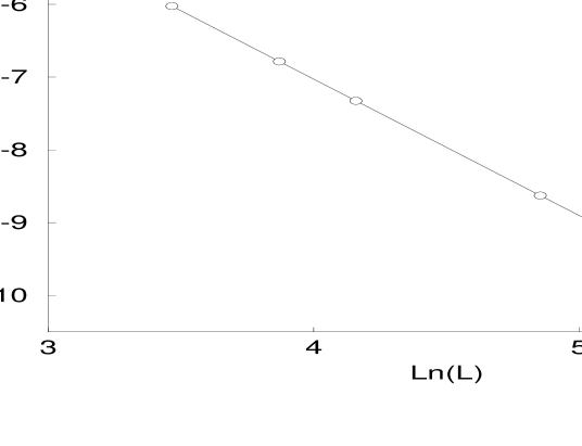
Figure 1: Scaling behaviour of the Yang–Lee edge at a typical critical $\beta$ value ($\beta=1.22$).

The analysis began with a rough search for the leading critical behaviour predicted by (8). An independent test was also made using the (less accurate) susceptibility data and (7). Both methods indicated critical behaviour setting in for $\beta$ $>$ $\sim$ $1.2$. In Fig. 1 we show a typical log–log plot of $z_{1}$ the Yang–Lee edge versus $L$. This is at a typical candidate value of the critical temperature ($\beta=1.22$). The errors are considerably smaller than the symbols. For example, at $\beta=1.22$ we found $z_{1}=0.0024136(7)$ and $0.00017902(6)$ at $L=32$ and $128$ respectively. The slope of Fig. 1 gives the effective leading index $\lambda_{\hbox{eff}}$ ignoring corrections. At $\beta=1.22$ this is $\lambda_{\hbox{eff}}=-1.8761(2)$ where the chi-squared per degree of freedom ($\chi^{2}/{\rm{dof}}$) for the linear fit shown is $0.85$. In Fig. 2(a) we display the result of such fits as a function of $\beta$. The effective exponent $\lambda_{\hbox{eff}}$ is just the slope of the log–log linear fit which should obtain if critical behaviour is present (ignoring logarithmic corrections). The corresponding $\chi^{2}/{\rm{dof}}$ for the linear fit is also shown. Acceptable values are only found for $\beta$ in excess of around 1.2. To quantify this statement we demand

$$\chi^{2}/{\rm{dof}}\leq 2.0$$ (12)

which means $\beta\raisebox{-3.22916pt}{ {\small\shortstack{$>$ \\ $\sim$}} }1.185$. We note that the corresponding values of $\lambda_{\hbox{eff}}$ ($\raisebox{-3.22916pt}{ {\small\shortstack{$<$ \\ $\sim$}} }-1.872(2)$) include that ($-15/8=-1.875$) corresponding to the KT prediction.

Fig. 2 is evidence for (i) the validity of FSS over a range of values $\beta\geq\beta_{c}\simeq 1.185$ and (ii) at $\beta_{c}$ the exponent $\lambda_{\hbox{eff}}$ very close to the expected KT value (-15/8). Observation (i) means that, as in the $XY$ case, the system remains critical for $\beta\geq\beta_{c}$ and (ii) is evidence that $\lambda$ is in fact -15/8 and the question of whether or not the step model belongs to the same universality class as the $XY$ model must now be answered by determination of the correction exponent $r$.

We therefore assume the behaviour (8) with $\lambda=-15/8$ at $\beta=\beta_{c}$. The expected leading behaviour is removed and linear fits to

$$\ln\left(z_{1}L^{15/8}\right)\quad\hbox{vs.}\quad\ln\ln L$$ (13)

performed. The results are shown in Fig. 3. Since the value $\lambda=-15/8$ ($\eta=1/4$) is only expected at $\beta_{c}$ these results can be used to identify the possible values of critical temperature and to test for the presence of logarithmic corrections as in the $XY$–model [1].

Applying the same criterion (12) as for the leading behaviour, we search for a range of $\beta_{c}$ values giving an acceptable fit. We find

$$1.195\leq\beta_{c}\leq 1.295\quad\hbox{and correspondingly,}\quad 0.009\geq r\geq-0.034\,.$$ (14)

The range of acceptable $r$ values includes that found [1] for the $XY$–model ($-0.023\pm 0.010$) and that corresponding to no logarithmic corrections ($r=0$). As in our previous work [1], this range excludes the prediction $r=-1/16$ coming from an approximate renormalisation group treatment of the $XY$–model [9]. Thus we conclude that the present data are compatible with the step model being in the same universality class as the $XY$–model. We do not, however, exclude other possibilities.

The susceptibility data are consistent with the above analysis. If one assumes the KT value of $\eta(\beta_{c})=1/4$, one can construct a so-called Roomany–Wyld beta function approximant [19] from the finite–size data and use its zero to locate $\beta_{c}$ [1]. These approximants, based on pairs of lattice size $L,L^{\prime}$, converge very rapidly [19]. We estimate $\beta_{c}=1.22\pm 0.02$. This last analysis of course neglects possible logarithmic corrections to scaling.

We have also studied the specific heat. As for the $XY$–model, the step model data show a broad peak with no obvious relationship to the position of the leading critical point. The finite–size dependence is not dramatic and is likely to be of little value in further elucidating the criticial behaviour. A related question is to what extent one can make use of the Fisher zeroes [16, 20], i.e. zeroes of the partition function in the complex $\beta$ plane at zero external magnetic field $h$. For both this and the $XY$–model, these are much harder to locate than the Lee–Yang zeroes and are consequently less accurately determined.

4 Conclusions

The use of finite–size scaling applied to Lee–Yang zeroes has allowed us to present detailed evidence of critical behaviour in the two-dimensional step (sgn $O(2)$ spin) model. The data are consistent with this model being in the same universality class as the $XY$– ( $O(2)$ spin) model. That is, it undergoes a Kosterlitz–Thouless type transition with susceptibility index $\eta({\beta_{c}})=1/4$ and we determine that $\beta_{c}$ lies in the range $1.195\leq\beta_{c}\leq 1.295$. With the available statistics, we found the logarithmic correction exponent to lie in the range $-0.034\leq r\leq 0.009$. This should be compared with our measurement for the $XY$ correction exponent [1], $-0.033\leq r\leq-0.013$ with which it is compatable. The step model results are however also compatable with no logarithmic corrections ($r=0$ corresponds to $\beta_{c}=1.21$ and $\chi^{2}/{\rm{dof}}=0.92$).

The Mermin–Wagner theorem [10] does not apply directly to the step model because of the discontinuous nature of the interaction hamiltonian. However, it has long been believed [4, 8] that if a phase transition does exist, it will not involve a phase with long range order. The evidence presented here supports this view.

This raises a question as to the nature of the mechanism driving the phase transition in the step model. The KT phase transition of the $XY$–model is understood to be driven by the binding/unbinding of topological solutions (vortices). However, the energetics of vortex formation are very different in the step model [11, 6, 8]. Since vortices with effectively zero excitation energy can be created at all non-zero temperatures, the usual KT argument does not naturally lead one to expect such a phase transition in the step model.

If this is indeed the case, some other driving mechanism must be responsible for any phase transition. It would then be remarkable if — as the evidence presented here indicates – both models belong to the one universality class.

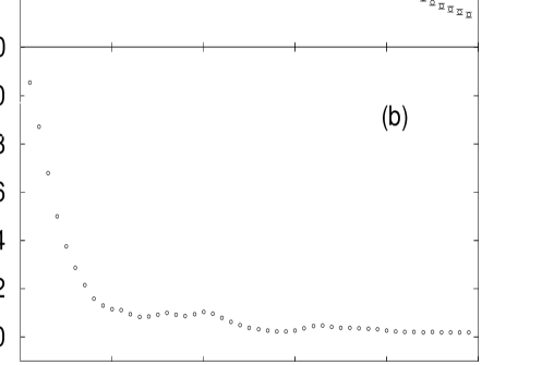
Figure 2: Test of expected leading critical behaviour: (a) the effective exponent $\lambda_{\rm{eff}}$ (slope of a straight line fit) and (b) the corresponding $\chi^{2}/{\rm{dof}}$ versus $\beta$.

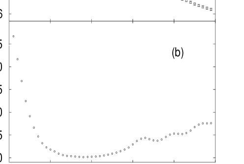
Figure 3: Logarithmic corrections: (a) the logarithmic correction exponent $r$ to the Yang–Lee edge is shown as a function of the assumed critical coupling $\beta_{c}$ and (b) the corresponding $\chi^{2}/{\rm{dof}}$.

References

- [1] R. Kenna and A. C. Irving, Phys. Lett. B 351, 273 (1995).
- [2] C. N. Yang and T. D. Lee, Phys. Rev. 87 404 (1952); ibid. 410.
- [3] A. J. Guttmann, G. S. Joyce and C. J. Thompson, Phys. Lett. A 38, 297 (1972).
- [4] A. J. Guttmann and G. S. Joyce, J. Phys. C 6, 2691 (1973).
- [5] I-H. Lee and R. E. Shrock, Phys. Rev. B 36, 3712 (1987).
- [6] I-H. Lee and R. E. Shrock, J. Phys. A 21, 2111 (1988).
- [7] A. Nymeyer and A. C. Irving, J. Phys. A 19, 1745 (1986).
- [8] E. Sánchez-Velasco and P. Wills, Phys. Rev. B 37, 406 (1988).
- [9] J. M. Kosterlitz and D. J. Thouless, J. Phys. C 6, 1181 (1973); J. M. Kosterlitz J. Phys. C 7, 1046 (1974).
- [10] N.D. Mermin and H. Wagner, Phys. Rev. Lett. 17 1133 (1966).
- [11] A. J. Guttmann and A. Nymeyer, J. Phys. A 11 1131 (1978).
- [12] F. Dunlop and C.M. Newman, Commun. Math. Phys. 44 223 (1975).
- [13] U. Wolff, Phys. Rev. Lett. 62 361 (1989).
- [14] A.M. Ferrenberg and R.H. Swendsen, Phys. Rev. Lett. 61 2635 (1988); Computers in Physics, Sep/Oct 1989.
- [15] K. Kajantie, L. Kärkkäinen and K. Rummukainen Nucl. Phys. B 357 693 (1991).
- [16] R. Kenna and C. B. Lang, Phys. Lett. B 264 396 (1991); Nucl. Phys. B (Proc. Suppl.) 30 697 (1993); Nucl. Phys. B 393 461 (1993); Err. ibid. B 411 (1994) 340.
- [17] R. Kenna and C. B. Lang, Phys. Rev. E 49 5012 (1994).
- [18] R. Kenna and A. C. Irving, Liverpool Preprint LTH 364.
- [19] M.P. Nightingale, Physica A 83 (1976) 561; H. Roomany and H.W. Wyld, Phys. Rev. D 21 (1980) 3341.
- [20] M.E. Fisher, in Critical Phenomena, Proc. 51th Enrico Fermi Summer School, Varena, ed. M.S. Green (Academic Press, NY, 1972).