A Study of Degenerate Four-quark states in SU(2) Lattice Monte Carlo

Abstract

The energies of four-quark states are calculated for geometries in which the quarks are situated on the corners of a series of tetrahedra and also for geometries that correspond to gradually distorting these tetrahedra into a plane. The interest in tetrahedra arises because they are composed of three degenerate partitions of the four quarks into two two-quark colour singlets. This is an extension of earlier work showing that geometries with two degenerate partitions (e.g. squares) experience a large binding energy. It is now found that even larger binding energies do not result, but that for the tetrahedra the ground and first excited states become degenerate in energy. The calculation is carried out using SU(2) for static quarks in the quenched approximation with $\beta=2.4$ on a $16^{3}\times 32$ lattice. The results are analysed using the correlation matrix between different euclidean times and the implications of these results are discussed for a model based on two-quark potentials.

I Introduction

In many-particle systems it is often convenient, or even necessary, to replace the fundamental two-particle interaction by an effective interaction, which can be very different from the original. For example, in metals the repulsive coulomb interaction between the valence electrons – because of the presence of the underlying ionic lattice – is replaced by an effective interaction that is attractive. Also in nuclei, the free two-nucleon potential gets strongly modified by the presence of the other nucleons. In both of these examples, after this removal of the explicit photon and meson degrees of freedom, the resultant effective interaction is still mainly in the form of a two-body interaction – with only a minor three-body term arising in the nuclear case. However, for a system of quarks interacting via gluon-exchange – even though this basic interaction is that of QCD – little is known in multiquark systems about the corresponding effective interquark interaction after the explicit gluon degrees of freedom have been removed. This is an important question, if realistic calculations are to be made for interacting quark clusters e.g. as in meson-meson, meson-nucleon or, eventually, nucleus-nucleus scattering. At present, the only way to carry out these fundamental calculations is by using Monte Carlo lattice techniques. Unfortunately, mainly due to the limitations of present day computers, these calculations are restricted to clusters of, at most, two or three quarks – see for example Ref. [1]. Therefore, a bridge is needed between lattice calculations involving few quarks and conventional many-body techniques that can accomodate larger numbers of quarks.

In an attempt to throw some light on the relationship between QCD and the effective interquark interaction, a series of model calculations have recently been made [2]–[8]. In these, the energies of four quarks in various configurations (e.g. on the corners of a rectangle or tetrahedron) have been calculated in quenched static SU(2) on a $16^{3}\times 32$ lattice. The reason for studying four quarks is because of the possibility for partitioning these into different colour-singlet groups each containing two quarks – a situation not possible with 2 and 3 quark systems. This can then be considered as a step towards the scattering of quark clusters – in this case meson-meson scattering. Hopefully, many of the features of an effective interquark interaction in SU(2) will be preserved in the more realistic case of SU(3) – in the same way as, for example, the ratios of glue-ball masses/string energy are numerically very similar in SU(2) and SU(3) [9]–[11].

In Refs. [3]–[8], the main feature in the results is that the strongest interaction between two separate two-quark clusters occurs when two of the three possible partitions of the clusters are degenerate, or almost degenerate, in energy. This was first observed in Ref. [3], where the four-quark binding energy $E$ dropped by an order of magnitude, when the four-quark geometry changed from that of a square [$r\times r$] to a neighbouring rectangle [$r\times(r\pm a)$] – where $r$ is the length of a side of the square in lattice units $a$. For example, $E(3a\times 3a)=-0.054(1)/a=-90$ MeV compared with $E(3a\times 2a\ {\rm or}\ 4a)\approx-0.006(1)/a$. Subsequent works verified this observation with other geometries, where the two partitions were not exactly degenerate – but more so than for the above rectangles. For example, in Ref. [5] this was achieved by tilting the rectangles out of the planes defining the underlying lattice, and also with other non-planar geometries. These latter cases showed that it was indeed the energy degeneracy dictating the size of the interaction and not a geometrical degeneracy. In other words, with clusters (13)(24) and interquark potentials $V(ij)$, it is the degeneracy $V(13)+V(24)\approx V(14)+V(23)$ that matters and not $|\mbox{\bf r}_{1}-\mbox{\bf r}_{3}|+|\mbox{\bf r}_{1}-\mbox{\bf r}_{3}|\approx|\mbox{\bf r}_{1}-\mbox{\bf r}_{4}|+|\mbox{\bf r}_{2}-\mbox{\bf r}_{3}|$. For large interquark distances $V(ij)\approx b_{s}|\mbox{\bf r}_{i}-\mbox{\bf r}_{j}|+c$, where $b_{s}$ is the string energy and $c$ an additive constant. In that case, the energy- and geometrical- degeneracy are the same. However, this is only true for $r_{ij}\geq 0.5$ fm and in the interesting region dominated by explicit quark interactions it is the energy degeneracy criterion that must be used. This is contrary to the assumption made with the so-called flip-flop model of Ref. [12] that takes the geometrical degeneracy criterion for all interquark distances.

The reason for studying many different 4-quark configurations (i.e. rectangles, linear, non-planar, etc.) is to give a representative selection of geometrical possibilities that arise in practice when, for example, two mesons scatter. Any quark model for such a scattering, when reduced to the same conditions as the lattice calculation [i.e. static, quenched, SU(2)] should give for the above selection of configurations the same values for the 4-quark energies $E$. As said earlier, the representative selection of 4-quark configurations concentrated on those cases where two of the three possible partitions were degenerate in energy. However, a potentially interesting case is that of the tetrahedron, where all three partitions are now degenerate. This is the main subject of this paper and is discussed in section 2. For completeness, the series of configurations shown in figure 1 are treated with $1\leq d\leq 5$ and $1\leq r\leq 6$ – the tetrahedron being $r=d$. The $r=1$ case is then closely related to the earlier work on squares with $d=1,\ldots,5$ and serves as a check on those calculations, since they were done with a set of basis states restricted to two in number and not three as in the present work.

Since the completion of Refs. [3]–[7], it has been suggested [13] that perhaps more care is needed in extracting energies and their statistical errors from a series of Monte Carlo results. Therefore, in section 3, the data is analysed taking into account data correlations between different euclidean times.

II The lattice Monte Carlo calculation

Since most of the details of the lattice Monte Carlo calculation have been given in the earlier papers [3]–[5], this section will only very briefly outline those details concentrating mainly on aspects specific to the geometry shown in Fig. 1.

Throughout this study the four quarks are treated in the static quenched approximation on a $16^{3}\times 32$ lattice in SU(2) with $\beta=2.4$ – corresponding to a lattice spacing of $a\approx 0.12$ fm. Both the four-quark energies $V_{i}(4q)$ and the corresponding two-quark energies $V_{i}(2q)$ are extracted on this lattice. However, the main quantities of interest are the ground state binding energy $E_{i=1}$ and the excited state energies $E_{i=2,3}$ defined by the differences

$$E_{i}=V_{i}(4q)-2V_{1}(2q)$$ (1)

As described in Refs. [3]–[5], the $V(2q)$ potentials are calculated from a 3*3 variational basis, where – after fixing the gauge so that all temporal links are set to unity – the three states are constructed from basic lattice links that have been “fuzzed” to different levels – 12, 16 and 20 in the spatial directions. This fuzzing essentially models a glue flux-tube between the two quarks in question. For the cases where these two quarks are not along a given spatial axis [e.g. $V(x,y)$], the appropriate path of links is then constructed as the average of the two most simple paths connecting $x$ and $y$ – each consisting of one straight section along the $x$ and $y$ axes. For $V(4q)$, using only the maximum fuzzing level of 20, the basis states are constructed from the different partitions of four quarks into a product of two two-quark colour-singlet clusters. In some cases it seems natural to restrict the variational basis to just two partitions e.g. with rectangles the two involving the sides of the rectangle and not the one constructed from the two diagonal paths. However, in other cases – especially for the tetrahedron of interest here – it is seems to be necessary to keep all three partitions.

Having constructed the above paths (e.g. $P_{i}(T_{1})=U_{i}(T_{1})|\mbox{Vac}\rangle$ and $P_{j}(T_{2})=U_{j}(T_{2})|\mbox{Vac}\rangle$) from fuzzy links, Wilson loops $W_{ij}^{T}$ – the quantities from which the final energies are extracted – are then simply given, with the present gauge, as the overlap of paths separated by euclidean time $T=T_{2}-T_{1}$ i.e. $W_{ij}^{T}=\langle P_{j}(T_{1}+T)|P_{i}(T_{1})\rangle$.

The energies $E_{i}$ in Eq. (1) are expected to be exact in the sense that they are not the result of a truncated weak or strong coupling expansion. However, they do contain uncertainties such as:

a) Statistical errors. To a large extent these can be estimated with reasonable accuracy – the subject of section 3.

b) Systematic errors. By their very nature they are much harder to estimate. Throughout, the aim is to attempt at minimizing their effect. In general, the most obvious source of such errors is the use of a lattice that is too small (i.e. too few points) or has a grid that is too coarse (i.e. $\beta$ too small) for the results to represent those expected in the continuum limit of the lattice. This was checked in Ref. [5] by using a $24^{3}\times 32$ lattice at $\beta=2.5$, which corresponds to a lattice spacing $a\approx 0.082$ fm. In the present type of calculation, since – as seen from Eq. (1) – the signal $E_{i}$ is a delicate cancellation, it is necessary to ensure that the appropriate $V_{i}(4q)$ and $V_{1}(2q)$ are extracted simultaneously from the same lattice configuration. In this way, systematic errors possibly present in the separate energies $V_{i}(4q)$ and $V_{1}(2q)$ are expected to cancel to some extent.

In order to study different aspects of degenerate geometries, three separate sets of lattice calculations are performed in this paper.

• 1. The first concentrates on geometries near to the tetrahedra – namely – those cases with $r=d,d\pm 1$ (except for $d=1$, where only $r=1,2$ are treated). The data is collected into 69 blocks each containing 32 measurements i.e. 2208 measurements in all.

  2. The second set of geometries is for $r=1$ and $d=2$ to 5 i.e. situations close to that of the squares studied earlier in Refs. [3]–[7]. Here the data is collected into 47 blocks each containing 64 measurements i.e. 3008 measurements in all.

  3. In order to see the connection between the present series of geometries – especially that in the previous item – and the square/rectangle geometry of Refs. [3]–[7], a third set of runs is carried out. These are a repeat of the earlier square/rectangle geometry but with the complete 3*3 basis i.e. with the inclusion of the basis state constructed from the diagonal paths. Only a limited number of 64 measurements are made – 4 blocks each containing 16 measurements. However, this is sufficient to see how the energies vary in going from the three 2*2 bases (A+B, A+C and B+C) to the complete A+B+C basis.

III Analysis of the data

As emphasized, for example, in Refs. [13]–[14], care should be taken when analyzing data generated in Monte Carlo lattice calculations, in case the data between different euclidean times is too correlated. This can be taken into account in the following manner. As discussed in the previous section, the actual quantities measured are the Wilson loops $W_{ij}^{T}$ between different states $i,j$ at different time intervals $T$. Here the $i,j$ refer to the different degrees of fuzzing for the two-quark potentials and, for the four-quark case, to the different quark partitions. However, the quantities of interest are the energies ($V$) of these systems. In Refs. [3]–[7] these were extracted by solving the eigenvalue equation

$$W_{ij}^{T}a_{j}^{T}=\lambda^{(T)}W_{ij}^{T-1}a_{j}^{T},$$ (2)

where $\lambda_{i}^{(T)}\rightarrow\exp(-V_{i})$ as $T\rightarrow\infty$. This matrix formulation takes into account mixing between the different degrees of fuzzing or four-quark partitions, but says nothing about possible correlations between the different times $T$. As suggested in Ref. [13] it is convenient to treat the configuration and time correlations in the same manner. For clarity, this is illustrated by the specific example of $n$ partitions and $T$ time differences in the four-quark case. This involves the $(n^{2}T)$ matrix elements $W_{11}^{T},W_{12}^{T},\ldots,W_{nn}^{T}$, where the expected equality between, for example, $W_{12}^{T}$ and $W_{21}^{T}$ is not enforced by symmetrizing the data. Let the index $p=1,\ldots,n^{2}$ denote these $n^{2}$ matrices. As discussed in the previous section, the data ($W_{ij}^{T}$) in the form of these $(n^{2}T)$ matrix elements is collected into $N$ separate blocks, each of which is already the average of $m$ measurements i.e. in all there are $mN$ measurements of each Wilson loop. The average of these measurements is denoted by

$$\bar{W}_{ij}^{T}=\frac{1}{N}\sum^{N}_{l=1}W_{ij}^{T}(l).$$ (3)

The problem is now reduced to fitting these averages by a function of the general form

$$F^{T}_{p}=\sum_{k=1}^{k_{M}}a_{p}(k)\exp(-V_{k}T)$$ (4)

in order to extract the energies $V_{k}$. As shown in Ref. [13] this can be achieved by minimizing the expression

$$\chi^{2}=\sum_{T,T^{\prime},p,p^{\prime}}\left(F^{T}_{p}-\bar{W}^{T}_{p}\right)M(T,T^{\prime},p,p^{\prime})\left(F^{T^{\prime}}_{p^{\prime}}-\bar{W}^{T^{\prime}}_{p^{\prime}}\right),$$ (5)

where

$$M(T,T^{\prime},p,p^{\prime})=NC^{-1}(T,T^{\prime},p,p^{\prime})$$ (6)

and $C$ is the covariance matrix

$$C(T,T^{\prime},p,p^{\prime})=\frac{1}{N-1}\sum_{l=1}^{N}\left(W_{p}^{T}(l)-\bar{W}_{p}^{T}\right)\left(W_{p^{\prime}}^{T^{\prime}}(l)-\bar{W}_{p^{\prime}}^{T^{\prime}}\right).$$ (7)

In what follows, it is convenient to introduce the correlation matrix

$$\tilde{C}(T,T^{\prime},p,p^{\prime})=\frac{C(T,T^{\prime},p,p^{\prime})}{\sqrt{C(T,T,p,p)C(T^{\prime},T^{\prime},p^{\prime},p^{\prime})}}$$ (8)

The above procedure is stable provided $N$ is large enough. However, in the present type of lattice calculation this is not guaranteed and can then lead to $\tilde{C}(T,T^{\prime},p,p^{\prime})$ having very small eigenvalues that produce large fluctuations in $M(T,T^{\prime},p,p^{\prime})$. As argued in Ref. [13], such eigenvalues correspond to eigenvectors that alternate in sign as a function of $T$ and so are not very relevant to smooth fit functions of the type proposed in Eq. (4). It is, therefore, reasonable to remove these disturbing eigenvalues and here the suggestion made in Ref. [13] is adopted. This simply replaces the smallest eigenvalues of $\tilde{C}(T,T^{\prime},p,p^{\prime})$ by their average. The question then arises concerning how many $(n_{t})$ of the original eigenvalues $(n_{T}=n^{2}T)$ should be retained. Initially a number $n_{M}$ of these $n_{T}$ eigenvalues are fixed – with $n_{M}$ being chosen as $\approx\sqrt{N}$ – a compromise choice found after some experimentation in Ref. [13]. The average $(\lambda_{av})$ of the remaining $n_{T}-n_{M}$ eigenvalues is then made and those eigenvalues less than $(\lambda_{av})$ are replaced by $(\lambda_{av})$ itself. Since only a fraction of the $n_{T}-n_{M}$ eigenvalues are replaced in this way, there still remains $n_{t}>n_{M}$ of the original eigenvalues. In practice the final value of $n_{t}$ is not strongly dependent on the original choice of $n_{M}$. In the present problem $N=69$, $n=2$ or 3 and $T$ can range from 1 to 5, so that for the largest $\tilde{C}$ matrix only about 8 of the total number of 45 original eigenvalues should be retained. However, frequently the $T=1$ data are dropped from the analysis, since they have very small error bars and presumably contain the effect of several higher energy components that become negligible already at $T=2$ and so cannot be seen for $T\geq 2$. Therefore, keeping the $T=1$ data often makes it difficult to obtain an accurate fit with only a few (1 – 3) terms $V_{i}$.

Having arrived at a suitable model for $\tilde{C}$, it remains to fix the precise form of the function $F^{T}_{p}$ in Eq. (4), which is to fit the $n^{2}T$ matrix elements $\bar{W}^{T}_{p}$ by means of Eq. (5). It is seen that the $F^{T}_{p}$ are described by the $k_{M}$ potentials $V_{k}$ and the corresponding $n^{2}k_{M}$ amplitudes $a_{p}(k)$ i.e. in all $(n^{2}+1)k_{M}$ parameters. For the four-quark case the most reliable fits are found with three partitions $(n=3)$ and four time steps $(T=2,\ldots,5)$, which means 36 pieces of data are to be fitted with $10k_{M}$ parameters. Therefore, in principle only three potentials $(V_{1,2,3})$ can at most be extracted. However, fitting 36 numbers (some having significant error bars) with 30 parameters ($k_{M}=3$) would not succeed. In fact, even the extraction of two potentials using the 20 parameters ($k_{M}=2$) would probably not give values of $V_{1,2}$ with a meaningful accuracy. It is, therefore, necessary to impose some theoretical constraints to restrict the number ($n^{2}k_{M}$) of parameters $a_{p}(k)$. Since the data $\bar{W}^{T}_{i,j}$ involve the overlap of two lattice configurations $P_{i}(0)=U_{i}(0)|\mbox{Vac}\rangle$ and $P_{j}(T)=U_{j}(T)|\mbox{Vac}\rangle$ separated by time $T$, it can be written as the vacuum expectation

$$\bar{W}^{T}_{i,j}=\langle\mbox{Vac}|U_{j}(T)U_{i}(0)|\mbox{Vac}\rangle=\sum_{k}\langle\mbox{Vac}|U_{j}(T)|k\rangle\langle k|U_{i}(0)|\mbox{Vac}\rangle\exp(-V_{k}T)$$ (9)

It is, therefore, reasonable to assume that the amplitudes are separable i.e. $a_{p}(k)=a_{ij}(k)=a_{i}(k)a_{j}(k)$. This has two good features:

1) The number of parameters is now reduced to $(n+1)k_{M}$. Therefore, fitting the 36 pieces of data from three partitions $(n=3)$ and four time steps now only requires $4k_{M}$ parameters. This makes the quite reliable extraction of two or possibly three potentials feasible.

2) This parametrisation imposes the symmetry $F^{T}_{ij}=F^{T}_{ji}$ as is expected physically. As said earlier this symmetry was not forced on the original data by some procedure such as taking the average $0.5(\bar{W}^{T}_{ij}+\bar{W}^{T}_{ji})$, since the differences between $\bar{W}^{T}_{ij}$ and $\bar{W}^{T}_{ji}$ can contribute to the error analysis of the extracted energies.

It should be added that, in the event of two energy states being degenerate (e.g. $V_{k_{1}}=V_{k_{2}}$), then $a_{i}(k_{1})a_{j}(k_{1})+a_{i}(k_{2})a_{j}(k_{2})$ should be replaced by a single amplitude $a_{ij}$. This is the situation encountered in the tetrahedron geometry. However, there additional symmetries suggest the following better model.

In some symmetrical cases, such as four quarks on the corners of a square or tetrahedron, the number of parameters can be further reduced by choosing forms of $F^{T}_{p}$ that guarantee various symmetries. For the square, when only the two partitions involving the sides are considered, the matrix of Wilson loops has the form

$${\bf W}^{T}=\left(\begin{array}[]{ll}W_{11}^{T}&W_{12}^{T}\\ W_{21}^{T}&W_{22}^{T}\end{array}\right),$$ (10)

where not only is the general symmetry $W_{12}=W_{21}$ expected but also for a square $W_{11}=W_{22}$. In this case Eq. (2) is easily solved to give for the lowest energy

$$\lambda_{1}=\frac{W^{T}_{11}+W^{T}_{12}}{W^{T-1}_{11}+W^{T-1}_{12}}$$ (11)

and for the energy of the first excited state

$$\lambda_{2}=\frac{W^{T}_{11}-W^{T}_{12}}{W^{T-1}_{11}-W^{T-1}_{12}}.$$ (12)

Therefore, in fitting the data it is reasonable to expect that only two potentials can be extracted i.e. $k_{M}=2$, and so the fitting functions must have the form

$\displaystyle F^{T}_{1}=F^{T}_{4}=a(1)\exp(-V_{1}T)+a(2)\exp(-V_{2}T)$

$$F^{T}_{2}=F^{T}_{3}=a(1)\exp(-V_{1}T)-a(2)\exp(-V_{2}T).$$ (13)

This reduces the number of parameters to four [$V_{1,2},a(1,2)$] in order to fit the 16 pieces of data covering four $T$ steps. Here it should be remembered that the suffix $p$ on $F^{T}_{p}$ is fixed as $p=j+n(i-1)$.

Similarly, for the tetrahedron the matrix of Wilson loops has the form

$${\bf W}^{T}=\left(\begin{array}[]{lll}W_{11}^{T}&W_{12}^{T}&W_{13}^{T}\\ W_{21}^{T}&W_{22}^{T}&W_{23}^{T}\\ W_{31}^{T}&W_{32}^{T}&W_{33}^{T}\end{array}\right),$$ (14)

where the general symmetries $W_{11}^{T}=W_{22}^{T}=W_{33}^{T}$, $W_{21}^{T}=W_{12}^{T}$, $W_{31}^{T}=W_{13}^{T}$, $W_{32}^{T}=W_{23}^{T}$ are expected and, in addition, there are the equalities $W_{13}^{T}=W_{12}^{T}$ and $W_{23}^{T}=-W_{13}^{T}$. The ”minus” sign appearing in the last equation is a reminder that the quarks are in fact fermions even though quarks and antiquarks transform in the same way under SU(2). This point is discussed in more detail in the appendix of Ref. [7]. Therefore, in all, there are only two independent Wilson loops $W_{11}^{T}$ and $W_{12}^{T}$. Again Eq. (2) is easily solved to give for the lowest energy (occurring twice)

$$\lambda_{1,2}=\frac{W^{T}_{11}+W^{T}_{12}}{W^{T-1}_{11}+W^{T-1}_{12}}$$ (15)

and for the excited state

$$\lambda_{3}=\frac{W^{T}_{11}-2W^{T}_{12}}{W^{T-1}_{11}-2W^{T-1}_{12}}.$$ (16)

In fitting the data it is reasonable to expect that only two terms can be extracted, i.e. $k_{M}=2$, and so the fitting functions must have the form

$\displaystyle F^{T}_{1}=F^{T}_{5}=F^{T}_{9}=a(1)\exp(-V_{1}T)+a(2)\exp(-V_{2}T)$

$$F^{T}_{2}=F^{T}_{3}=F^{T}_{4}=F^{T}_{7}=-F^{T}_{6}=-F^{T}_{8}=\\ 0.5a(1)\exp(-V_{1}T)-a(2)\exp(-V_{2}T).$$ (17)

This again reduces the number of parameters to four [$V_{1,2},a(1,2)$] in order to fit the 12 pieces of data $(n=3)$ covering four $T$ steps. In this case, due to the high symmetry there are no longer 36 pieces of independent data.

In the tetrahedral case it is also seen that, when one of the partitions is removed (i.e. $n$ drops from 3 to 2), the Wilson loop matrix reduces to the same form as that in Eq. (10). As seen by comparing Eqs. (11) and (15) the lowest eigenvalue is now the same in the $n=2$ and 3 cases. However, the first excited state is quite different in the two cases – unlike the result for most other geometries. For example, as will be seen later in Table IV of Section IV, for squares and for those rectangles so far discussed, the $n=2$ and 3 cases give very similar results for $E_{2}$ as well as $E_{1}$. However, there the third partition has a higher energy than the other two partitions, whereas for the tetrahedron all three partitions have the same energy. When the tetrahedron is distorted into a neighbouring lattice configuration, it will be seen in Table II of Section IV that both $E_{1}$ and $E_{2}$ can again be given quite accurately by $n$=2. It should be added that for very elongated rectangles the two partitions with the highest energy become more and more degenerate. In that case $E_{1}$ is essentially zero and $E_{2}$ will depend more and more on the presence of the third partition.

In an idealised situation, all of the available $n^{2}$ pieces of data from $T$=1 to 5 should – using the above procedure – be fitted with a $F^{T}_{p}$ containing $k_{M}\approx n$ potentials. This would then be the natural extension of Eq. (2) for incorporating into its $n$ eigenvalues the effects of correlations between different values of $T$. As it now stands that equation only includes the mixing between the different fuzzing levels or partitions. However, in practice, fitting all the $T$ values is not possible and decisions have to be made concerning both the data ($\bar{W}^{T}_{ij}$) to actually be fitted and, in the fitting procedure, the form of $F^{T}_{p}$ and also the model for the correlation matrix in Eq. (8).

a) In the present problem, the data goes from $T$=1 to 5 and the number ($n$) of fuzzings (2-quark) or partitions (4-quark) can range from 1 to 3. For both the 2- and 4- quark systems usually $T$=2 to 5 turns out to be the most suitable range. When the $T$ range is reduced to 3–5, better values of $\chi^{2}$ emerge from Eq. (5) but at the expense of larger errors on the extracted potentials $V_{i}$. On the other hand, when $T=1$ data is included – because of the small errors on this new data – it usually results in either a “no-solution” situation or a $\chi^{2}$ that is too large to be meaningful. In addition to the restriction on $T$, a decision must be made on the number of fuzzings or partitions to be included. In the 2-quark system only two fuzzings were necessary at a given time. This is simply a reflection that the different degrees of fuzzing are effectively very similar and so little is gained by increasing the number of different fuzzings from 2 to 3. Here the two largest fuzzing levels (16 and 20) are used i.e. $n$ is always taken to be two in the 2-quark case. In the 4-quark case it is possible to use all of the data from the different partitions i.e. $n$ is always three in the tetrahedron case.

b) In $F^{T}_{p}$, once the separable form or the more symmetrical one in Eqs. (13) or (17) have been chosen, the only decision to be made is the value of $k_{M}$ – the number of terms $(V_{i})$ to be determined. This is varied between 1 and 3. In the correlation matrix $\tilde{C}(T,T^{\prime},p,p^{\prime})$ of Eq. (8) the number of eigenvalues to be initially retained ($n_{M}$) can also be varied. Ref. [13] suggests using $n_{M}\approx\sqrt{N}$, and this was found to be a suitable value in the four-quark case as can be seen from Table I (there $N=69$, so that the $\sqrt{N}$-result is shown as case 11). On the other hand, in the two-quark system it is necessary to use $n_{M}=2$ or 3 to get a stable fit. Table I shows the effect of varying $n_{M}$ in a four-quark system (cases 9–13), as well as a fit with no correlations (i.e. $\tilde{C}={\bf 1}$, case 8). A few general features can now be seen:

1. Comparing cases 8 and 11, the use of the correlation matrix has approximately a one-sigma-level effect on the averages and it slightly decreases the errors.

2. The exact value of $n_{M}$ is not important as long as approximately all the stable eigenvalues are retained (i.e. $n_{t}$ is in the right range). To estimate this range for $n_{t}$ a jackknife procedure on the eigenvalues was carried out[15].

The above choices in the data and fitting procedure are strongly inter-related and so a strategy is necessary to single out the optimal set of values for $n$, the range of $T$, $k_{M}$ and $n_{M}$. An example of this is given in Table I. Basically this strategy amounts to first fitting only a portion of the data e.g. $T=$(3 or 4) – 5, with only a few potentials e.g. $k_{M}=$1 or 2 – see cases 1–2 in Table I. It is possible to see a suitable range for $n_{t}$, and therefore for $n_{M}$ as well, already from these fits. Then $k_{M}$ is increased to find a maximum number of potentials that can be extracted by using this range of $T$ (see cases 2,6,7). The data base is then progressively enlarged to include more timesteps, while trying to keep the value of $\chi^{2}$ per degree of freedom fixed or decreasing by adding more potentials if possible (cases 2–7). Naturally, adding a timestep constrains the potentials more than before, so that the errors of the potentials decrease accordingly. Initially this works well, but eventually the $\chi^{2}$ become larger and larger, so that usually the results become meaningless before the ultimate stage of including all of the data (i.e. $n=3$ and $T=$1 – 5). However, it should be added that the $T=1$ data fitted with $k_{M}=3$ has to be treated with caution, if the resulting potentials are significantly different from those extracted with $T=2-5$ and $k_{M}$=2, since this may indicate that even higher energy states are polluting the $T=1$ data.

IV Results

The results for the tetrahedron-like geometry in Fig. 1 are shown in Fig. 2 and Tables II and III. Several points arise from Table II:

• 1. From earlier work in Refs. [3]–[5], for the corresponding squares [i.e. $(d,0)$ in this notation], where two of the basis states are degenerate, the binding energy of the lowest state ranges from –0.07 to –0.05 as $d$ goes from 1 to 5 [see Table IV]. However, now – even though at least two of the basis states are always degenerate ($A$ and $B$) – the ground state binding energy is always less than that of the corresponding square [$E_{1}(d,0)$]. For a fixed $d$, $|E_{1}(d,r)|$ decreases as $r$ increases. Nothing interesting happens to $E_{1}$ at $r=d$, at which point all the basis states are degenerate in energy.

  2. For fixed $d$, as $r$ increases from 0 to $d$, the energy of the first excited state $E_{2}$ decreases until $E_{2}(d,d)=E_{1}(d,d)$. For $r>d$, $E_{2}(d,r)$ increases again. This degeneracy of $E_{1,2}$ for the tetrahedron is a new feature compared with earlier geometries. As will emerge in the next section, this is a severe constraint on any model wishing to describe this data.

  3. As seen from columns $A+B+C\ (I\ {\rm and}\ II)$, in all cases the energies extracted using either ($I$) Eqs. (5)–(8) or ($II$) Eq. (2) are within the error bars of each other. If a choice has to be made, then the results $(I)$ are prefered, since they involve a more detailed analysis of the data.

  4. In columns $A+B$ and $B+C$ only the corresponding two basis states are used. The symbol $S$ means that the extracted $E_{1}$ are exactly the same as the $A+B+C(II)$ results. In those cases it is, therefore, sufficient to only use a 2*2 basis. However, the choice of which 2*2 basis depends on the particular geometry, since one of these two basis states must have the lowest unperturbed energy. Since $A$ and $B$ are degenerate in energy, for a given $d$ this amounts to using $A+B$ for $r\leq d$. Whereas, for $r>d$ it is necessary to use $B+C$, since $C$ now has the lowest unperturbed energy.

  5. Except for the tetrahedra, the values of $E_{2}$ are essentially the same in the 2*2 and 3*3 bases.

  6. The values of $E_{3}(d,r)$ are always much higher than $E_{2}(d,r)$. However, as discussed in the next section, this second excited state is dominated by excitations of the gluon field and so is outside the scope of the models introduced in that section.

  7. The last column shows the two 2-quark ground state potentials $V_{1}(d,d)$ and $V_{1}(d,r)$ that enter with this geometry. In the next section, these are needed for evaluating a model for the 4-quark binding energies.

Several of the above points are also illustrated in Fig. 2 for the case of $d/a=3$ and $r/a=0,1,2,3,4$. In addition, there are shown the theoretical predictions for the $f=1$ limit of the model to be discussed in the next section.

Table III is very similar to Table II except that $r/a$ is now restricted to unity i.e. geometries nearest to the $(d\times d)$ squares. The following points can be made:

• 1. Again the energies extracted by Eqs. (5)–(8) ($I$) and Eq. (2) ($II$) are within the error bars of each other – with ($I$) being preferable, since it involves a more detailed analysis of the data.

  2. For comparison in $E_{i}(d\times d)$ are given the energies of the nearby squares from Ref. [5] with only a 2*2 basis but analysed with method $(I)$. In general, these all have a somewhat larger binding energy, indicating that the binding energy is maximized for the square geometry.

In Table IV results are given for various square/rectangle geometries. The main purpose of this set of runs is to see any change in the results for $E_{1,2}$ extracted from the 2*2 bases, when this is extended to a 3*3 basis by including a third state $C$. Also an estimate can now be made for the position of the second excited state $E_{3}$.

Several comments should be made about these results

• 1. For the lowest energy $E_{1}$, introducing the third basis state has little effect on the results given by the two basis state calculation provided the partition with the lowest energy is one of those two states in that basis. In fact, for squares (i.e. $r=d$) the results are identical for the $A+B+C$ and $A+B$ bases. However, in a general case when using a 2*2 basis, for $d>r$ it is necessary to include state $A$ and for $d<r$ state $B$. Remember that in this notation it is state $C$ that is constructed from the diagonal two-quark colour singlets and so always has the highest unperturbed energy.

  2. The energy $E_{2}$ of the first excited state is less dependent on the choice of basis – with the 3*3 and 2*2 possibilities giving in most cases essentially the same results.

  3. From column $A+B+C$ it is seen that $E_{3}$ – the energy of the second excited state – is always considerably higher in energy than $E_{2}$.

  4. The $E_{i}(P)$ column is the result of many more measurements than the following columns. Therefore, in view of the facts in the previous items, these numbers should be considered as the most accurate for rectangles. They are basically the same as those in refs. [4], [5] and [7], except that the data has been subjected to the improved analysis ($I$) using Eqs. (5)–(8).

V An interpretation of the results

One of the main reasons for embarking on this work is the attempt to find a model which gives a simple understanding of the four-quark binding energies in terms of the corresponding two-quark potentials. At first sight, it may seem that the best such model should be able to explain all of the energies extracted from the lattice calculation of the previous section. However, this would be not only too ambitious but also it would be outside of the goal of the desired model. When the lattice data is analysed by directly diagonalizing Eq. (2), then the number of energies extracted is equal to the number of basis states i.e. three for the tetrahedral geometry. On the other hand, when the expression in Eq. (5) is minimized, the number of extracted energies depends very much on the quality of the lattice data. For the tetrahedron, as seen in Tables II–III, it is also possible to extract the three lowest eigenvalues and, in principle, even more could be obtained. This point is discussed in more detail in ref. [16], where also the results from other four-quark geometries are extracted using Eqs. (5)–(9). However, for the model to be discussed below only the lowest two lattice eigenvalues are of interest, since the third is dominated by excited gluon components. Such a feature is outside any model that incorporates an interaction that is based on the two-quark potential in its ground state. It can be seen that the third state is basically a gluonic field excitation as follows:

1) As shown in the above tables and also in the appendix of Ref. [7], except for the tetrahedra, the addition of a third basis state into the lattice calculation has only a minor effect on the results using only two basis states – indicating that the structure of the third eigenstate is very different from the lower two states.

2) In the linear case, on a lattice where all three partitions are constructed from links along a single spatial axis, i.e. without the need for introducing combinations of links along different axes, these partitions are linearly dependent leading to a singular matrix, if a three basis calculation is attempted in Eq. (2).

The previous paragraph has shown that only the lowest two lattice eigenvalues are of interest when constructing a model based on the basic two-quark potential in its ground state. To this end, in refs.[3]–[7] it was proposed that the lattice energies $E_{i}$ should be fitted by a model defined in terms of only two basis states $A$ and $B$. In this model the $E_{i}$ are given as the eigenvalues of the equation

$$\left[{\bf V}(f)-\lambda_{i}(f){\bf N}(f)\right]\Psi_{i}=0,$$ (18)

with

$${\bf N}(f)=\left(\begin{array}[]{ll}1&f/2\\ f/2&1\end{array}\right)\ \ {\rm and}\ \ {\bf V}(f)=\left(\begin{array}[]{cc}v_{13}+v_{24}&fV_{AB}\\ fV_{BA}&v_{14}+v_{23}\end{array}\right),$$ (19)

where $\lambda_{i}=E_{i}+v_{13}+v_{24}$ – the configuration $A=(q_{1}\bar{q}_{3})(q_{2}\bar{q}_{4})$ being the lowest in energy of the three possible partitions into two two-quark singlets. The off-diagonal matrix element

$$\langle A|V|B\rangle=V_{AB}=V_{BA}=\frac{1}{2}\left(v_{13}+v_{24}+v_{14}+v_{23}-v_{12}-v_{34}\right)$$ (20)

is of the form expected from a two-quark isovector potential

$$V_{ij}=-\frac{1}{3}{\bf\tau}_{i}\cdot{\bf\tau}_{j}v_{ij}.$$ (21)

The additional factor of $f$ appearing in the off-diagonal matrix elements is to be interpreted as a gluon field overlap factor. In the weak coupling limit $f$ is unity. However, in general this limit is found to result in too much binding compared with the lattice results. Therefore, $f$ is treated as a phenomenological factor, which is adjusted to fit the lattice energies. The problem is then reduced to understanding the resulting values of $f$, which have essentially simply replaced the lattice energies. That this is a reasonable model is supported by several points:

• 1. This factor $f$ is approximately unity when all four quarks are close together. This is indeed where the $f=1$ weak coupling limit should be best.

  2. For a given geometry, a single value of $f$ qualitatively explains quite well both $E_{1}$ and $E_{2}$.

  3. When $f$ is parametrized as

     $$f=\exp[-kb_{s}S],$$ (22)

     where $S$ is the minimal area of a surface bounded by the straight lines connecting the four quarks and $b_{s}a^{2}$ is the string energy density with the value $\approx 0.070$, then it is found that – for squares and rectangles – the parameter $k$ is reasonably constant at $\approx 0.50\pm 0.05$. Of course, the ultimate goal is to find such a parametrization in which the corresponding parameter(s) $k$ would be strictly constant for all geometries (i.e. squares, tetrahedra,$\ldots$). If this selection of geometries is sufficiently representative, then the reasonable assumption would be that this same parametrization should work for other geometries not calculated on the lattice.

Prior to this work on tetrahedrons the geometries considered had, at most, two of the three possible partitions being degenerate in energy (e.g. for squares). In these cases, as seen from Table IV, it is found that the lattice energies $E_{1}$ and $E_{2}$ are essentially the same for the three-basis-state calculation $(A+B+C)$ and those two-basis-state calculations ($A+B,\ A+C$ and effectively $B+C$) which involve the basis state with lowest unperturbed energy. This is one of the reasons why the 2*2 version of the $f-$model in Eq. (19) was quite successful for a qualitative understanding of these cases. However, for tetrahedra and the neighbouring geometries calculated in Section 2, it now seems plausible to extend the $f$-model to the corresponding 3*3 version in which

$${\bf N}(f)=\left(\begin{array}[]{lll}1&f/2&f^{\prime}/2\\ f/2&1&-f^{\prime\prime}/2\\ f^{\prime}/2&-f^{\prime\prime}/2&1\end{array}\right)\ \ {\rm and}\ \ {\bf V}(f)=\left(\begin{array}[]{ccc}v_{13}+v_{24}&fV_{AB}&f^{\prime}V_{AC}\\ fV_{BA}&v_{14}+v_{23}&-f^{\prime\prime}V_{BC}\\ f^{\prime}V_{CA}&-f^{\prime\prime}V_{CB}&v_{12}+v_{34}\end{array}\right),$$ (23)

where the negative sign in the BC matrix elements is of the same origin as the one in Eq. (14). This extension has both good and bad features. On the positive side, all three basis states are now treated on an equal footing. This is convenient when considering some general four-quark geometry, since it is then not necessary to choose some favoured 2*2 basis, which could well change as the geometry develops from one form to another. On the negative side, in the weak coupling limit (i.e. $f,f^{\prime},f^{\prime\prime}\rightarrow 1$) the 3*3 matrix of Eq. (18) becomes singular – in the sense that adding columns $B$ and $C$ results in column $A$. However, in this limit, each of 2*2 matrices corresponding to the three possible partitions A+B, A+C and B+C gives the same results. Away from weak coupling the 3*3 matrix is no longer singular, but now the three possible 2*2 partitions do not necessarily give the same results. Below an attempt is made to minimize the differences between these three partitions, since in the corresponding lattice calculation the differences in most cases are indeed small.

The strategy of trying to mimic the lattice calculation by means of the $f$-model in Eqs. (18) and (19) is carried out at two different levels.

• 1. The lattice calculation is made in the static quenched approximation with the SU(2) gauge group. Therefore, in the $f$-model there must not be any kinetic energy term (i.e. static quarks) and also quark-antiquark pair creation (for example in the form of meson exchange between quark clusters) must not be included (i.e. the quenched approximation). Furthermore, the two-quark potential in Eq. (21) is expressed in terms of $\tau$-matrices – the generators of SU(2).

  2. The lattice calculation, as said earlier, gives essentially the same results for any of the three partitions A+B, A+C and B+C as the complete A+B+C basis. As will be seen below, this point is more difficult to mimic. Since this feature is automatically encoded in the matrix elements of Eq. (14), one possibility for the $f$-model is to attempt to mimic in more detail the form of these matrix elements.

For the tetrahedron geometry, the $f$-model as written in Eq. (23) takes on a particularly simple form since each of the $v_{ij}$ are equal and also $f=f^{\prime}=f^{\prime\prime}$. In this case the eigenvalues are

$$E_{1}=E_{2}=E_{3}=0.$$ (24)

This has the positive feature that $E_{1}$ and $E_{2}$ are degenerate as in the lattice results of Table II. However, they are degenerate at zero binding energy. This latter feature is unavoidable for the model in its present form, since there is only one energy scale present. This is the two-quark potential between each of the quarks, which is, of course, independent of the pair of quarks chosen, since all interquark distances are the same for the tetrahedron. It is, therefore, necessary to introduce a second energy scale into the model. However, any improvements in the model have very limited choices, since there are only two different matrix elements involved – the diagonal ones all equal to $-E$ and the off-diagonals ones all equal to $\pm 0.5fE$. Therefore, the most general modifications are to change the diagonal matrix elements to $d_{1}-E$ and the off-diagonal ones to $\pm 0.5f(d_{2}-E)$. This results in the eigenvalues

$$E_{1}=E_{2}=\frac{d_{1}+0.5fd_{2}}{1+0.5f}\ \ {\rm and}\ \ E_{3}=\frac{d_{1}-fd_{2}}{1-f}.$$ (25)

At first sight it may appear that there is sufficient information to now extract the new parameters $d_{1,2}$, since $f$ can be estimated using the parameters (assumed to be universal) from other geometries – thus leaving two equations for $E_{1,2}$ and $E_{3}$ and the two unknowns $d_{1,2}$. However, as said before, this is too much to demand from the $f$-model, since in the lattice calculation the third basis state in the complete A+B+C basis generally plays a minor role in determining the values of $E_{1,2}$ and, therefore, the third eigenvalue is presumably dominated by an excitation of the gluon field. Even so, it is of interest to see that a similar feature now arises with $E_{3}$ in Eq. (25), since this third state is removed in the weak coupling limit i.e. $E_{3}\rightarrow\infty$ as $f\rightarrow 1$. However, the $f$-model – if it is to be successful – should only be expressed in terms of the lowest energy gluon configurations, since the gluon field is not explicitly in its formulation, but only appears implicitly in the form of the two-quark potentials and the $f$-factors. In view of this, no quantitative attempt should be made to identify the second excited state emerging from the lattice calculation as $E_{3}$ in the $f$-model.

In Ref. [17] it was shown that the two-state model of Eqs. (19) with the overlap factor $f=1$ agreed with perturbation theory upto fourth order in the quark-gluon coupling [i.e. to $O(\alpha^{2})$] and gives $E_{1,2}$=0 for tetrahedra. Therefore, the non-zero lattice results for small tetrahedra must be of $O(\alpha^{3})$ at least. Another aspect of this special situation for tetrahedra is also seen – when extracting or interpreting the value of $E_{2}$ – by the need for the third basis state both in the lattice calculation (see Table II) and in the $f$-model, since in comparison with Eq. (25) the two basis state version gives

$$E_{1}=\frac{d_{1}+0.5fd_{2}}{1+0.5f}\ \ {\rm and}\ \ E_{2}=\frac{d_{1}-0.5fd_{2}}{1-0.5f}$$ (26)

i.e. both the two- and three- basis state models have the same ground state, but the latter does not show the $E_{1}=E_{2}$ degeneracy.

In Fig. 2 the predictions are shown for the $f=1$ limit of the above model in the case of $d=3$. If, in the notation of Fig. 1, the appropriate two potentials in state $A$(or $B$) and state $C$ are defined as $v_{a}=V_{1}(3,r)$ and $v_{c}=V_{1}(3,3)$, respectively, then

$$V_{1}(4q)=\frac{8v_{a}-2v_{c}}{3}\ \ {\rm and}\ \ V_{2}(4q)=2v_{c}.$$ (27)

Here the $V_{i}(4q)$ are defined in Eq. (1). To extract $E_{i}$ for $r\leq d$ the two-quark potential $V_{1}(2q)$ is taken to be $v_{a}$, whereas for $r>d$ the appropriate potential is $V_{1}(2q)=v_{c}$.

The expressions in Eq. (25) are not particularly useful unless there is a model for the parameters $d_{1,2}$. However, since it’s not the purpose of this paper to make a comprehensive study of models covering all the 4-quark geometries considered in earlier works [4]–[8], only a few general remarks will be made here for the tetrahedron geometry. Models for the $d_{1,2}$ need extensions of the potential in Eq. (21), so that for the tetrahedron there are two energy scales present. Here several ways of achieving this goal are suggested:

• 1. The effect of an isoscalar two-quark potential.

     As discussed in Ref. [4], an isoscalar potential $w_{ij}$ can be introduced into $V_{ij}$ – ensuring $V_{ij}=v_{ij}$ for a colour singlet two-quark system – by the form

     $$V_{ij}=-\frac{1}{3}{\bf\tau}_{i}\cdot{\bf\tau}_{j}\left(v_{ij}-w_{ij}\right)+w_{ij}.$$ (28)

     In this case, $d_{1}=d_{2}=4w$ since all of the $w_{ij}$ are now equal to $w$ and results in $E_{1}=E_{2}=E_{3}=4w$. Therefore, from Table IV it is seen that the $w$ range from –0.0035 to –0.0070 i.e. they have values much smaller than the corresponding $v_{ij}=v$ given in the last column. A similar feature was found in Ref. [4], when the form in Eq. (28) was introduced to improve the model fit for squares and rectangles. However, as shown in Ref. [17], in perturbation theory all terms of $O(\alpha^{2})$ are included in the two state model of Eq. (19) with $f=1$. Therefore, in the weak coupling limit $w_{ij}$ must be of $O(\alpha^{3})$ at least.

  2. The effect of a three- or four-body potential.

     The $f$ factor is itself a four-body operator. However, it is conceivable that additional multiquark effects arise. Some perturbative possibilities are discussed in Ref. [17]. There it is shown that all three-quark terms arising from three gluon vertices always vanish, but that the four gluon vertex can contribute to 2-, 3- and 4-quark terms at $O(\alpha^{3})$. However, in the tetrahedral case ($r=d$), cancellations result in this particular 4-quark term also vanishing.

  3. The effect of non-interacting three gluon exchange processes.

     These are also discussed qualitatively in Ref. [17] and contribute at $O(\alpha^{3})$ to 2-, 3- and 4-quark potentials.

  4. The effect of two quark potentials in which the gluon field is excited.

     The first excited state [$V_{1}^{*}(r)$] of the two-quark potential $V_{1}(r)$ is approximately given by $V_{1}^{*}(r)\approx V_{1}(r)+\pi/r$ – see for example refs. [9, 10]. Therefore, if a fourth state – based on such an excited state – is introduced into the model, since it is higher in energy than the three degenerate basis states so far considered, it will give attraction in the ground state. Furthermore, as the size of the tetrahedron increases this fourth state will approach the other three states, so that the attraction felt in the ground state will increase – a trend seen in the tetrahedron results for $E_{1,2}$ in Table II.

The above isoscalar potential option now offers a reason for $E_{1}=E_{2}\not=0$. But, unfortunately, $E_{3}$ is still equal to $E_{1,2}$ since $d_{1}=d_{2}$. However, there is no reason to expect any three or four body forces to also be purely isoscalars. In this case, their contributions to $d_{1}$ and $d_{2}$ could be different and through the presence of the $1-f$ factor in Eq. (25) any estimates of $E_{3}$ could be very model dependent.

VI Conclusions

This paper discusses three separate aspects of four-quark energies:

1) Four-quark configurations (tetrahedra) involving three degenerate basis states.
This showed the interesting result that – for tetrahedra – the ground and first excited states are degenerate in energy. The onset of this degeneracy can be seen in Fig. 2, where – as a square ($r=0$) gets deformed into a tetrahedron ($r=d=3$) – the ground and first excited states, originally at –0.053 and 0.116, become degenerate at –0.026. This is a new feature not observed in earlier four-quark configurations (e.g. squares, linear,$\ldots$).

2) The use of the correlation matrix in euclidean time for extracting energies from the basic lattice data.
Because the four-quark binding energy is the difference of two quantities that are comparable in magnitude, the final result involves a rather delicate cancellation – see Eq. (1). It was, therefore, considered worth while to investigate the effect of correlations in the basic data. Here it is shown that such an improved analysis of the lattice data leads to results that are essentially the same as those in earlier, less complete, analyses.

3) The construction of a model in an attempt to explain these energies.
Here it is seen that the $f$-model, introduced in earlier papers, needs to be modified before it can be used to described the tetrahedron results. Hopefully, a guide to these modifications can be suggested by perturbation theory, which has already proven useful in justifying the basic model at small interquark distances.

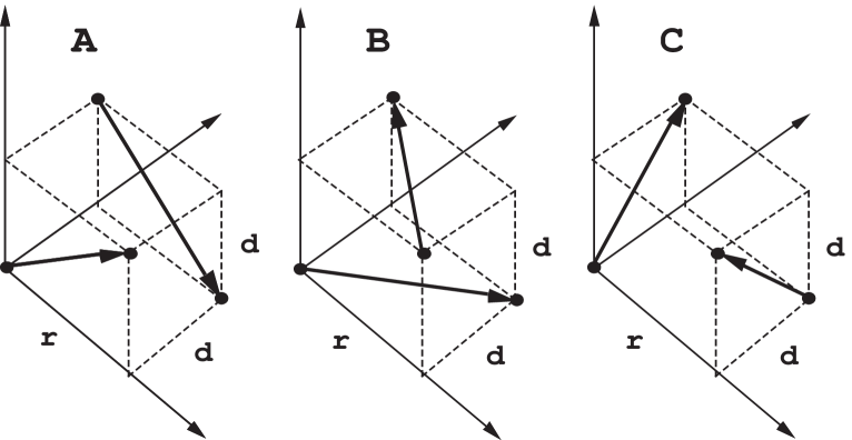
FIG. 1.: The four-quark geometry based on a square of side $d$ parallel to the $yz$-plane and a distance $r$ from that plane. $A,B$ and $C$ are the three possible partitions. The case when $r=d$ is called the tetrahedron.

FIG. 2.: The binding energies – in units of the lattice spacing – of the four-quark states for the geometry of Fig. 1 for $d=3$ and $r=0,1,2,3,4$.
Solid lines show lattice results:
$\diamond$ – the ground-state binding energy $E_{1}$.
$\times$ – the first excited state energy $E_{2}$.
Dashed and dotted lines show model results with $f=1$ from Eq. (27) for $E_{1}$ and $E_{2}$ respectively.

TABLE I.: The binding energies $E_{k}(d=3a,r=4a)$ obtained with method (I) from Eqs. (5)–(8).
$k_{M}$ is the number of energies extracted.
$T$ is the time range analysed.
$n_{M}$ is the number of eigenvalues initially retained.
$n_{t}$ is the actual number of unchanged eigenvalues finally retained using $n_{M}$.
$\chi^{2}$/DoF is the ratio of Chi-squared/Degrees of Freedom with the actual result shown in the parentheses.
Case 8 is a fit with a unit correlation matrix and is equivalent to the usual Least Squares fit.

Case	$k_{M}$	$T$	$n_{M}$	$n_{t}$	$E_{k}$			$\chi^{2}$/DoF
1	2	4–5	12	15	–0.06(3)	0.10(4)		230/10 (23)
2	3	4–5	12	15	–0.03(3)	0.07(4)	0.4(2)	3.9/6 (0.6)
3	3	3–5	10	16	–0.009(6)	0.097(8)	0.37(3)	8.9/15 (0.6)
4	3	2–5	8	17	–0.009(2)	0.105(2)	0.400(7)	12/24 (0.5)
5	3	1–5	8	16	–0.003(2)	0.116(2)	0.424(2)	100/33 (3.0)
6	4	2–5	8	17	–0.010(3)	0.097(7)	0.40(3)	10/20 (0.5)
					23.405(2)
7	4	1–5	8	16	–0.004(195)	0.108(36)	0.424(95)	43/29 (1.5)
					1.8(6.1)
8	3	2–5	–	–	–0.0100(19)	0.1035(25)	0.393(14)	8.8/24 (0.4)
9	3	2–5	0	7	–0.0091(19)	0.1045(23)	0.398(10)	10/24 (0.4)
10	3	2–5	2	11	–0.0090(17)	0.1053(24)	0.399(7)	10/24 (0.4)
11	3	2–5	8	17	–0.0090(17)	0.1054(23)	0.400(7)	12/24 (0.5)
12	3	2–5	15	22	–0.0091(17)	0.1054(22)	0.400(7)	16/24 (0.7)
13	3	2–5	36	36	–0.0087(17)	0.1065(19)	0.400(5)	28/24 (1.2)
14	method (II)				–0.010(2)	0.105(5)	0.39(3)	–

TABLE II.: The binding energies $E_{i}$ of four quarks in the geometry of Fig. 2 for $d=1$ with $r=1,2$ and $d=2,\ldots,5$ with $r=d,d\pm 1$. Here $r=d$ are the tetrahedra.
1) $A+B+C$ (I) is from Eqs. (5)–(9) with $A,B,C$ shown in Fig. 2.
2) $A+B+C$ (II) is from Eq. (2) in a 3*3 basis – see Ref. [7].
3) $A+B$ and $B+C$ are from Eq. (2) using only 2*2 bases
4) $V_{1}$ are the two-quark potentials i) $V_{1}(d,d)$ and ii) $V_{1}(d,r)$
5) The symbol S indicates that the entry in the table is the same as that to its left – within numerical accuracy i.e. rounding errors.
These results are from 2208 measurements contained in 69 blocks of 32 measurements each.

$(d/a,r/a)$	$E_{i}$	$A$+$B$+$C$ (I)	$A$+$B$+$C$ (II)	$A$+$B$	$B$+$C$	$V_{1}$
(1,1)	$E_{1}$	–0.0145(4)	–0.016(2)	S	S	i)	0.4885(1)
	$E_{2}$	”	”	–0.016(2)	–0.016(2)
	$E_{3}$	0.85(2)	0.834(4)
(1,2)	$E_{1}$	–0.0034(4)	–0.003(1)	0.03(1)	S	i)	0.4885(1)
	$E_{2}$	0.262(2)	0.265(2)	0.265(2)	0.262(2)	ii)	0.6023(3)
	$E_{3}$	0.95(9)	0.849(3)
(2,1)	$E_{1}$	–0.0453(9)	–0.043(2)	S	–0.042(2)	i)	0.6689(4)
	$E_{2}$	0.083(2)	0.085(2)	0.086(2)	0.084(2)	ii)	0.6023(3)
	$E_{3}$	0.78(7)	0.67(3)
(2,2)	$E_{1}$	–0.0202(8)	–0.020(1)	S	S	i)	0.6689(4)
	$E_{2}$	”	”	–0.017(2)	–0.017(2)
	$E_{3}$	0.524(6)	0.49(3)
(2,3)	$E_{1}$	–0.010(2)	–0.008(2)	–0.002(4)	–0.008(1)	i)	0.6689(4)
	$E_{2}$	0.147(3)	0.147(2)	0.147(2)	0.150(5)	ii)	0.7421(6)
	$E_{3}$	0.60(3)	0.58(2)
(3,2)	$E_{1}$	–0.040(1)	–0.041(1)	S	–0.33(3)	i)	0.7974(8)
	$E_{2}$	0.050(1)	0.048(2)	0.053(4)	0.050(5)	ii)	0.7421(6)
	$E_{3}$	0.443(6)	0.41(3)
(3,3)	$E_{1}$	–0.026(1)	–0.028(1)	S	S	i)	0.7974(8)
	$E_{2}$	”	”	–0.006(4)	–0.006(4)
	$E_{3}$	0.367(7)	0.366(6)
(3,4)	$E_{1}$	–0.009(1)	–0.010(2)	0.025(9)	–0.008(1)	i)	0.7974(8)
	$E_{2}$	0.106(1)	0.105(5)	0.105(5)	0.12(1)	ii)	0.8589(11)
	$E_{3}$	0.400(6)	0.39(3)
(4,3)	$E_{1}$	–0.036(2)	–0.039(2)	S	–0.016(2)	i)	0.9102(15)
	$E_{2}$	0.033(2)	0.03(1)	0.03(2)	0.04(1)	ii)	0.8589(11)
	$E_{3}$	0.326(6)	0.34(1)
(4,4)	$E_{1}$	–0.028(3)	–0.033(3)	S	S	i)	0.9102(15)
	$E_{2}$	”	”	0.021(2)	0.021(2)
	$E_{3}$	0.270(9)	0.26(1)
(4,5)	$E_{1}$	–0.009(3)	–0.012(2)	0.089(4)	–0.008(5)	i)	0.9102(15)
	$E_{2}$	0.089(3)	0.089(4)	0.089(5)	0.13(1)	ii)	0.967(2)
	$E_{3}$	0.298(7)	0.31(1)
(5,4)	$E_{1}$	–0.025(5)	–0.04(1)	S	0.03(2)	i)	1.017(2)
	$E_{2}$	0.025(5)	0.023(5)	0.05(1)	0.02(3)	ii)	0.967(2)
	$E_{3}$	0.24(1)	0.24(1)
(5,5)	$E_{1}$	–0.017(8)	–0.10(4)	S	S	i)	1.017(2)
	$E_{2}$	”	”	0.044(8)	0.44(8)
	$E_{3}$	0.19(1)	0.19(1)
(5,6)	$E_{1}$	–0.06(3)	–0.013(4)	0.00(6)	–0.011(4)	i)	1.017(2)
	$E_{2}$	0.01(5)	0.0(1)	0.0(1)	0.03(7)	ii)	1.072(4)
	$E_{3}$	0.15(9)	0.14(10)

TABLE III.: The notation is the same as Table II but with $r=1$ and $d=2,3,4,5$
These results are from 3008 measurements contained in 47 blocks of 64 measurements each.
The $E_{i}(d\times d)$ are the corresponding energies for the nearby square of side $d$.

$(d/a,r/a)$		$A$+$B$+$C$ (I)	$A$+$B$+$C$ (II)	$E_{i}(d\times d)$	$V_{1}$
(2,1)	$E_{1}$	–0.0447(6)	–0.043(2)	–0.0588(3)	i)	0.6689(4)
	$E_{2}$	0.085(1)	0.085(1)	0.1414(8)	ii)	0.6021(3)
	$E_{3}$	0.69(3)	0.66(3)
(3,1)	$E_{1}$	–0.052(2)	–0.049(2)	–0.0531(5)	i)	0.7974(8)
	$E_{2}$	0.089(3)	0.09(1)	0.1157(12)	ii)	0.6992(5)
	$E_{3}$	0.53(2)	0.55(5)
(4,1)	$E_{1}$	–0.050(4)	–0.047(1)	–0.0524(10)	i)	0.9102(15)
	$E_{2}$	0.088(6)	0.088(3)	0.097(2)	ii)	0.7841(10)
	$E_{3}$	0.54(5)	0.54(3)
(5,1)	$E_{1}$	–0.052(5)	–0.044(5)	–0.047(3)	i)	1.017(2)
	$E_{2}$	0.073(8)	0.073(1)	0.075(3)	ii)	0.8652(8)
	$E_{3}$	0.51(9)	0.55(4)

TABLE IV.: The energies for a selection of squares and rectangles in the ranges $d=1,\ldots,5$ and $r=1,\ldots,5$.
The $E_{i}$ are from a 2*2 basis using 800(1600) for the rectangles(squares). In contrast to Ref. [7], these results utilize Eqs. (5)–(9) and not Eq. (2).
The other columns use only 64 measurements.
$A+B+C$ denotes the 3*3 basis and $A+B,\ \ B+C$ the corresponding 2*2 bases.
The energies are those at $T=3$ and not from any plateau in $T$.
The notation is that:
$A$ has links along the sides of length $r$.
$B$ has links along the sides of length $d$.
$C$ is the state defined by the diagonals.
$S(L)$ is the state(s) with the lowest unperturbed energy.

$(d/a,r/a)$		$E_{i}(P)$	$A+B+C$	$A+B$	$A+C$	$S(L)$
(1,1)	$E_{1}$	–0.0694(5)	–0.0694(3)	S	S
	$E_{2}$	0.1828(7)	0.1841(11)	0.1842(11)	0.1846(11)	$A,B$
	$E_{3}$	-	0.974(25)	–	–
(1,2)	$E_{1}$	–0.0029(2)	–0.00150(18)	–0.00148(17)	–0.00075(16)
	$E_{2}$	0.504(2)	0.5074(19)	0.5077(20)	0.5089(20)	$B$
	$E_{3}$	-	1.037(19)	–	–
(2,1)	$E_{1}$	–0.0029(2)	–0.00165(38)	–0.00163(38)	–0.00164(38)
	$E_{2}$	0.504(2)	0.5080(28)	0.5083(29)	0.511(3)	$A$
	$E_{3}$	-	1.027(26)	–	–
(2,2)	$E_{1}$	–0.0588(3)	–0.0574(13)	S	–0.0566(14)
	$E_{2}$	0.1414(8)	0.1429(14)	0.1433(13)	0.1496(7)	$A,B$
	$E_{3}$	-	0.766(18)	–	–
(2,3)	$E_{1}$	–0.0052(4)	–0.0038(11)	–0.0038(11)	+0.0019(14)
	$E_{2}$	0.325(1)	0.324(4)	0.324(4)	0.329(4)	$B$
	$E_{3}$	-	0.807(12)	–	–
(3,2)	$E_{1}$	–0.0052(4)	–0.0044(3)	–0.0043(3)	–0.0044(2)
	$E_{2}$	0.325(1)	0.326(3)	0.326(3)	0.342(3)	$A$
	$E_{3}$	-	0.776(17)	–	–
(3,3)	$E_{1}$	–0.0531(5)	–0.0538(16)	S	–0.0493(19)
	$E_{2}$	0.1157(12)	0.1113(27)	0.1112(27)	0.130(4)	$A,B$
	$E_{3}$	-	0.661(19)	–	–
(3,4)	$E_{1}$	–0.0041(6)	–0.0039(17)	–0.0039(17)	+0.018(3)
	$E_{2}$	0.253(1)	0.255(15)	0.255(15)	0.260(14)	$B$
	$E_{3}$	-	0.705(29)	–	–
(4,3)	$E_{1}$	–0.0041(6)	–0.0070(22)	–0.0071(22)	–0.0072(22)
	$E_{2}$	0.253(1)	0.261(7)	0.262(7)	0.290(4)	$A$
	$E_{3}$	-	0.73(5)	–	–
(4,4)	$E_{1}$	–0.0524(10)	–0.0466(56)	S	–0.032(5)
	$E_{2}$	0.097(2)	0.087(12)	0.088(12)	0.124(16)	$A,B$
	$E_{3}$	-	0.59(7)	–	–
(5,5)	$E_{1}$	–0.047(3)	–0.026(10)	S	–0.001(12)
	$E_{2}$	0.075(3)	0.088(10)	0.092(12)	0.136(13)	$A,B$
	$E_{3}$	-	0.87(5)	–