BROWN-HET-984

BU-CCS-950602

May 1995

Monte Carlo Study of the Yukawa Coupled

Two Spin Ising Model

Richard Brower^a, Kostas Orginos^b, Yue Shen^a and Chung-I Tan^b

^aDepartment of Physics, Boston University, Boston, MA 02215
^bDepartment of Physics, Brown University, Providence, RI

1 Introduction

It often happens in quantum field theory that exactly the same physical system can be described by very different actions. For example, the critical behavior of a two dimensional paramagnetic film can be described either by a Bosonic 2d Ising model, or equivalently by a 2d free Fermion field [1]. Another example is the exact equivalence of Sine-Gordan theory and the massive Thirring model. Kinks in the elementary scalar field theory become elementary Fermions while the scalars are composite Fermion anti-Fermion bound states[2].

A similar equivalence exists for the Goldstone modes of chiral symmetry breaking which can be described either in terms of an elementary scalar field theory or as composite scalar modes in a Fermion-antiFermion channel. For example it has been shown that the Higgs-Yukawa model and the generalized Nambu-Jona-Lasinio Model [3] are identical. Note that in the last example, the number of degrees of freedom appears to be very different at the cut-off scale, yet the low energy physics turns out to be exactly the same. All of these are manifestations of the the well known universality property: different microscopic Lagrangians can lead to the same continuum theory (critical behavior) as long as the fixed point structure and the low mass excitations of the two actions are the same.

Here we wish to consider a different but closely related phenomenon where the same excitation is represented twice in a single Lagrangian by two different fields, yet in the scaling limit the theory is universal to either spin system taken separately. Such a redundant description has recently been advocated as an improved lattice formulation of GCD in the so called chirally extended action (XQCD)[4],[5]. Here an elementary scalar field is coupled to the Wilson lattice QCD action. It was conjectured that XQCD is in the same universality class as the Wilson lattice QCD action and its critical property describes the continuum QCD physics. An obvious problem for XQCD is the extra degrees of freedom introduced by the scalar fields on the lattice. Will the extra degrees of freedom decouple in the continuum limit? This question can not be answered easily without nonperturbative calculations.

An important feature of this suggestion is the existence of a global (Higgs) symmetry G in each field theory so that the combined theory has a $G\times G$ symmetry that is broken down to $G$ by a Yukawa coupling. In these more complicated examples, it is not obvious when they remain in the same universality class as the original theory or if numerical methods can give convincing evidence. We were able to prove that an extended Nambu-Jona Lasino model and a two spin coupled O(N) models are equivalent in large N [4, 5]. At large N, the extra degrees of freedom become decoupled in the continuum limit and the low energy spectrum is exactly the same as if no extra degrees of freedom were introduced at the cut-off scale. Our purpose in this article is to begin the use of numerical methods to supplement analytical methods. To this end we consider a simple model of redundant coupled Ising spins to see if Monte Carlo methods can settle the question of universality and expose the mechanism by which it is achieved in the scaling limit.

2 Yukawa Coupled Spin Ising Model

For the our two spin Ising system, we consider the action,

$$S=-\kappa_{1}\sum_{x,\mu}\sigma_{x+\mu}\sigma_{x}-\kappa_{2}\sum_{x,\mu}s_{x+\mu}s_{x}-y\sum_{x}\sigma_{x}s_{x}~{},$$ (1)

where $\sigma_{x}=\pm 1$ and $s_{x}=\pm 1$. The sum over $x=(n_{1},n_{2})$ is performed on a two dimensional lattice, $n_{i}=1,2,\cdots,L$, with nearest neighbor couplings, $\mu=(1,0),\;(0,1)$. A very general class of four spins models could be considered. Our particular choice we call a “Yukawa” coupling borrowing terminology from field theories for spontaneous breaking of continuous symmetry. When the Yukawa coupling y is set to zero, this model (1) reduces to two independent 2d Ising models with a global $Z_{2}\times Z_{2}$ symmetry. But when $y$ is different from zero, only a single $Z_{2}$ symmetry is survives. This is a special example of 4 state spin models, which to our knowledge has no analytic solution. It is no longer self-dual.

At the cut-off scale there are two fields, $\sigma_{x}$ and $s_{x}$, in the coupled Ising model in Eq. (1). However, as we will show in the following sections, only one eigenvalue of the mass matrix remains in the spectrum in the continuum limit. The other mass eigenvalue stays at the cut-off scale. We believe that the light mass corresponds to the massive particle of a 2d Ising model. We will further show that the coupled Ising model follows the scaling laws of a 2d Ising model. Therefore, our model in Eq. (1) is in the same universality class of a 2d Ising model.

Admittedly in this case the universality of our 4 state spin model to the Ising model is not surprising. The Yukawa coupled two spin model is in fact nothing but an Ising model written on 3-d lattice with only two layers in the third axis and three independent couplings: $\kappa_{1}$ and $\kappa_{2}$ in each x-y layer and $y$ along the z axis. Since this model can be viewed as a $d=2+\epsilon$ model with vanishing $\epsilon$ in the thermodynamic limit and since other anisotropic Ising models are known to be in the isotropic Ising universality class, universality with a single Ising spin system appears likely . When we tune to the critical surface and the correlation length $\xi$ becomes much larger than $2$, the system should behave like a single layer 2d Ising model. Still it is important for our larger purposes to see if numerical methods can give convincing evidence and that analysis of the spectrum can illuminate the mechanism for approaching the single spin system in the scaling limit. Finally we should note that since the totally decoupled system ($y=0$) is clearly not a single Ising system, so one expects that by carefully tuning the Yukawa term a new interacting two spin fixed point must also exist which is not universal to a single spin system. This fine tuning limit is what is often required to obtain a true 2 Higgs system in the continuum.

3 Phase Diagram

First we need to determine the phase diagram of the model. For arbitrary $\kappa_{1}$, $\kappa_{2}$ and $y$, Eq. (1) describes a two layered Ising model with different couplings in each layer. In general, we expect that the magnetization in one layer will induce the magnetization in the second layer when the coupling between layers, $y$, is nonzero. Therefore, the size of the symmetric region,as shown in Figure 1, will be reduced. A few limiting cases can be easily derived.

If $y\neq 0,\kappa_{2}=0,\kappa_{1}\neq 0$, the sum over $s_{x}$ can be carried out explicitly

$$Z = \sum_{\{\sigma\}}\sum_{\{s\}}e^{\textstyle\kappa_{1}\sum_{x,\mu}\sigma_{x}\sigma_{x+\mu}+y\sum_{x}\sigma_{x}s_{x}}$$

$$= \sum_{\textstyle\{\sigma\}}\;\;e^{\textstyle\kappa_{1}\sum_{x,\mu}\sigma_{x}\sigma_{x+\mu}}e^{\sum_{x}ln[ch(y\sigma_{x})]}$$

$$= const\times\sum_{\{\sigma\}}e^{\textstyle\kappa_{1}\sum_{x,\mu}\sigma_{x}\sigma_{x+\mu}}~{},$$

Thus the model becomes the standard 2d Ising model and the critical point is known from the exact solution $\kappa_{1,cr}=\kappa_{c}=0.44068...$. It is also easy to show that a spontaneous symmetry breaking in $\sigma$ will induce a magnetization in $s$

$$<s>=tanh(y)<\sigma>~{},$$ (4)

where $<\sigma>$ is given by the 2d Ising model solution. Similar result can be derived for $\kappa_{1}=0,\kappa_{2}\neq 0,y\neq 0$.

In the limit $y\to\infty$, $\sigma_{x}$ would be completely aligned with $s_{x}$, and up to a constant the action can be written as

$$S=-(\kappa_{1}+\kappa_{2})\sum_{x,\mu}\sigma_{x}\sigma_{x+\mu}~{}.$$ (5)

This is again a 2d Ising model with critical point given by a straight line,

$$\kappa_{1}+\kappa_{2}=\kappa_{c}=0.44068...~{},$$ (6)

in the $\kappa_{1}-\kappa_{2}$ phase plane. At finite $y$, the phase boundary lies between the limit of $y=0$ and $y\to\infty$ as shown in Figure 1. It was determined using Monte Carlo simulations which were carried out on a 64-node CM-5 at Boston university. For simplicity, we have used the heat-bath algorithm. The size of lattices we used range from $16^{2}$ to $128^{2}$. The phase boundary was determined by observing the magnetization, defined as:

$$<m_{1}>=<\left|{1\over L^{2}}\sum_{x}\sigma_{x}\right|>,\ \ \ \ <m_{2}>=<\left|{1\over L^{2}}\sum_{x}s_{x}\right|>~{}.$$ (7)

It is non-vanishing on a finite lattice in both phases, but will converge to the physical magnetization in the infinite volume limit. Near the phase transition point, $<m_{1}>,<m_{2}>$ changes rapidly from finite values to almost zero in the symmetric phase. This cross-over behavior becomes sharper with increasing lattice size. The results for $y=0.50$ are shown in Figure 1. The points have been computed while the line is a simple interpolation. ¿From this figure one can get that $y=0.50$, $\kappa_{2}=0.20$ and $\kappa_{1}=0.325(5)$ is a critical point. This point will be used in the study of the propagators.

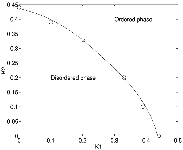
Figure 1: Phase diagram for $y=0.50$. The lattice size is $32^{2}$. The solid line is an interpolation to the points.

For a more precise measurement of the critical point, we used the Binder index [6]

$$U_{1}(L)=1-{<m_{1}^{4}>\over 3<m_{1}^{2}>^{2}}~{},\ \ \ \ U_{2}(L)=1-{<m_{2}^{4}>\over 3<m_{2}^{2}>^{2}}~{}.$$ (8)

For the simplest case $\kappa_{1}=\kappa_{2}=y/2=\beta$, we have $U_{1}=U_{2}\equiv U(L,\kappa)$. When the volume is large, $U(L,\kappa)$ should cross at an unique point $(U^{*},\kappa_{c})$. However, for practical $L$ and $L^{\prime}$, the crossing point depends on the ratio $s=L^{\prime}/L$ due to residual finite size corrections. We obtained the crossing point for a series of values of $s$, and fitted to the form [6]

$${1\over\beta}={a\over ln(s)}+{1\over\beta_{c}}~{},$$ (9)

as shown in Figure 2. We found $\beta_{c}=0.2759(2)$.

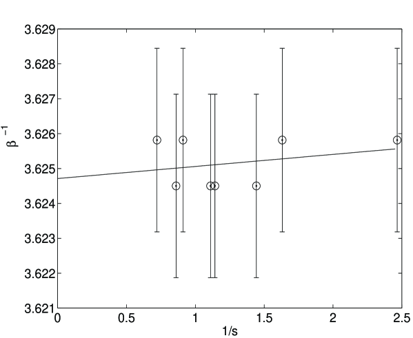
Figure 2: Determination of the critical point using the finite size scaling of the Binder Index. The fitting curve is $1/\beta=a/s+1/\beta_{c}$ ($s=log(L1/L2)$). The computed values of the fitting parameters are: $\beta_{c}=0.2759(2)$ and $a=0.000(2)$.

Another way to locate the critical point is to use the finite size scaling behavior of the susceptibility [7] [9]. We fitted the location of the peak ($\beta_{max}$) of susceptibility to:

$${1\over\beta_{max}}={1\over\beta_{c}}+{c\over L^{1\over\nu}}~{},$$ (10)

with $\nu=1$ (see next section). We found (see Figure 3) $\beta_{c}=0.2766(4)$, which is consistent with the result obtained using the Binder index.

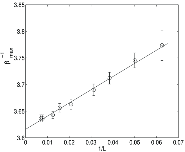
Figure 3: Location ($\beta_{max}$) of the Susceptibility Maximum vs. $L^{-\nu}$. Using Eq.10 ($1/\beta_{max}=1/\beta_{c}+a/L^{-\nu}$ ) we compute the critical point $\beta_{c}=0.2766(4)$. ($\nu$ is assumed to be $\nu=1$)

To be conservative, we take the difference in the above two estimates as an indication of the true error and quote the critical point to be $\beta_{c}=0.2759(7)$.

As an aside, we would like to point out that our model can also be used to test a very interesting method for computing critical points that has be suggested recently [8]. This method is based on the assumption that the critical point of a system in $d$ dimensions is located at the maximum of

$$\rho(\beta)=\lim_{L\rightarrow\infty}\left({(Tr{\cal T})^{2}\over Tr{\cal T}^{2}}\right)^{\textstyle L^{1-d}},$$ (11)

where $\cal T$ and ${\cal T}^{2}$ are the transfer matrices for the $d~{}-~{}1$ dimensional system and two coupled $d~{}-~{}1$ dimensional system respectively. It has been shown that the above method is valid for self-dual models. However, for non self-dual models it remains a conjecture. Unfortunately, we found from our simulations that the critical point of the two layered Ising model is $\beta_{c}=0.2759(7)$ so that it does not appear to agree with the critical point obtained in Ref [8].

4 Critical Indices

To establish the universality class, we need to investigate the finite size scaling (FSS) [9][7] behavior and determine the critical indices.

For $\kappa_{1}=\kappa_{2}=y/2=\beta$, we determine $\nu$ using

$${dU_{L}\over d\beta}=(1-U_{L})\left(<E>-2{<m^{2}E>\over<m^{2}>}+{<m^{4}E>\over<m^{4}>}\right)~{},$$ (12)

where $E$ is the Ising energy per site. At $\beta_{c}$, $dU_{L}/d\beta$ should scale as $L^{1/\nu}$. As shown in Figure 4, if we take $\beta_{c}=0.2759$, we find $\nu=0.99(3)$. This is to be compared with the exact value $\nu=1$ for the 2d Ising model.

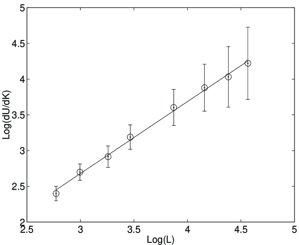
Figure 4: From the finite size scaling of ${dU_{L}\over d\beta}\sim L^{1/\nu}$ one obtains the critical exponent $\nu=0.99(3)$.

Next we measured the magnetization at the critical point $\beta_{c}=0.2759$. Fitting to the scaling form

$$m\sim L^{-\beta/\nu}~{},$$ (13)

as shown in Figure 5, we get $\beta/\nu=0.124(2)$. This should be compared to the exact value of 0.125

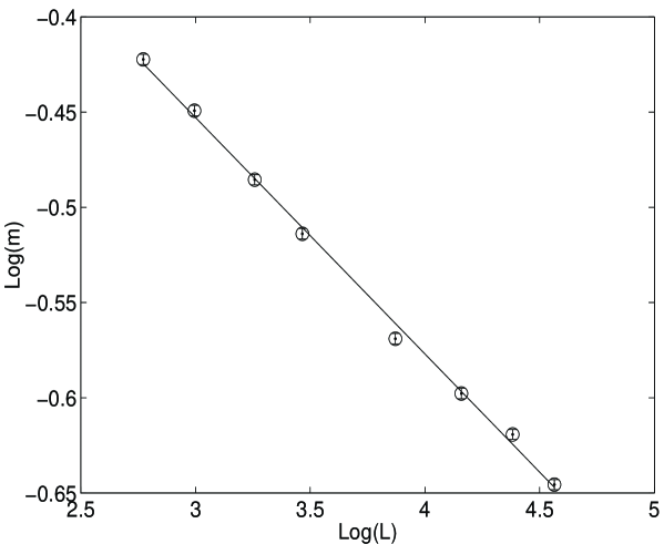
Figure 5: From the finite size scaling of $M\sim L^{\beta/\nu}$ one obtains $\beta/\nu=0.124(2)$.

To get the anomalous dimension, $\eta$, we measured the value of the susceptibility at $\beta_{c}=0.2759$ as a function of $L$ and fitted to the form

$$\chi_{max}\sim L^{2-\eta}~{}.$$ (14)

As shown in Figure 6, we found $\eta=0.27(6)$ in comparison to the exact value of 0.25.

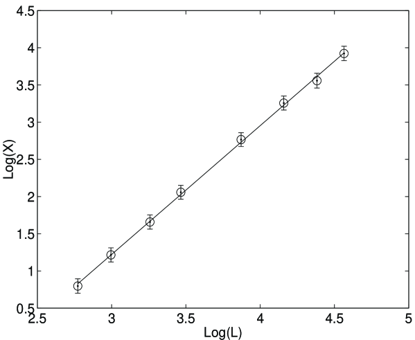
Figure 6: From the finite size scaling of $X\sim L^{2-\eta}$ one obtains the anomalous dimension $\eta=0.27(6)$.

All the results on the critical exponents are summarized in Table 1. The rest of the critical indices can be computed through scaling laws [9] $\alpha=2-\nu d$ , $\gamma/\nu=2-\eta$ , $\delta=(d+2-\eta)/(d-2+\eta)$. Thus we conclude that all the critical indices of our model are the same as those of the 2d Ising model. Consequently these two models are in the same Universality class and they have to the same continuum limit: a 2d free Fermion system [10].

Critical Exp.	2d Ising Model	2d Coupled Ising Model
$\nu$	1	0.99(3)
$\beta\over\nu$	0.125	0.124(2)
$\eta$	0.25	0.27(6)
$\alpha$	0	0.02(6)
$\delta$	15	14(3)
$\gamma\over\nu$	1.75	1.73(6)

Table 1: The critical exponents of the 2d Ising model and the coupled 2d Ising model. They seem to be identical with in the accuracy of our computation.

5 Mass Spectrum

We have established that the coupled Ising model in Eq. (1) and the 2d Ising model obey the same finite size scaling laws and therefore belong to the same universality class. However the mass spectrum still remains a puzzle. Although there are two fields $\sigma_{x}$ and $s_{x}$, we would like to know if there is one or two particles in the low energy spectrum.

Let us introduce the Fourier transformation of the fields as

$$\sigma(p)={1\over L^{d/2}}\sum_{x}\sigma_{x}e^{-ipx}~{},$$ (15)

$$s(p)={1\over L^{d/2}}\sum_{x}s_{x}e^{-ipx}~{}.$$ (16)

The propagators in Fourier space can be written as

$$G(p)=\left(\begin{array}[]{cc}<\sigma(p)\sigma(-p)>&<\sigma(p)s(-p)>\\ <s(p)\sigma(-p)>&<s(p)s(-p)>\\ \end{array}\right)~{}.$$ (17)

Near $p^{2}=0$, the two-point function can be expanded as

$$G^{-1}(p)=A+Bp^{2}+O(p^{4})~{},$$ (18)

where $A$ and $B$ are two-by-two matrices. $B$ leads to a wavefunction renormalization. Thus the matrix $M=B^{-1}A$ is the mass matrix. The eigenvalues of $M$ are the masses of the model (Here for simplicity, we define the masses at the zero momentum instead of the pole of the propagator).

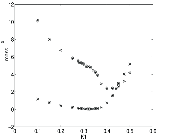
Figure 7: The mass matrix eigenvalues at $\kappa_{2}=0.20$ and $y=0.50$. One goes to zero while the other remains finite at the critical point $\kappa_{1}=0.325$. The mass unit is $1/a$.

Numerically, we have found that it is fairly easy to fit $G^{-1}_{\sigma\sigma}(p)$, $G^{-1}_{ss}(p)$ near $p^{2}=0$ to a linear form, and $G^{-1}_{\sigma s}(p)$ is essentially independent of $p^{2}$. We have obtained matrices $A$ and $B$ in Eq. (18) for $y=0.50$ , $\kappa_{2}=0.20$ and for various values of $\kappa_{1}$ so that we cross the phase boundary. The results for mass eigenvalues are shown in Figure 7. It is very clear that while the small mass eigenvalue goes to zero at the critical point, the heavy mass stays at $O(1)$ in lattice unit. We also fitted the light mass eigenvalue to the scaling form

$$m^{2}\sim(\kappa-\kappa_{c})^{1/\nu}~{},$$ (19)

and found that for $\nu=1$ one gets a very good fit of the data. (see Figure 8.) The deviation form the linear fit close to the critical point is due to FSS effects. This is another indication that the critical exponent $\nu$ is indeed $1$ as for the 2d Ising model.

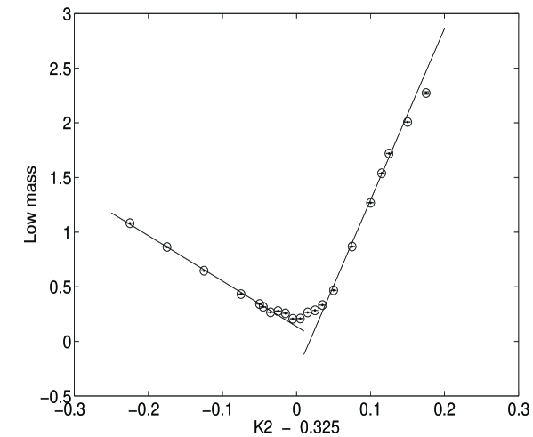
Figure 8: The linear fitting of the low mass around the critical point confirms the fact that $\nu$ is $1$. The mass unit is $1/a$.

From the analysis of the propagator, we can learn two important things: (1) only one particle remains in the physical spectrum even though there appears to be extra degrees of freedom at the cut-off scale; (2) the physical field is a linear combination of bare fields $\sigma_{x}$ and $s_{x}$.

6 Conclusions

In this paper we have studied a 2d spin model composed of two Ising systems interacting through a Yukawa coupling. There were two main objectives of our effort. One was to show that this form of coupling leads to the same universality class as a single 2d Ising model; the other was to show that only a single set of spin waves survives in the continuum limit. Our study of the critical exponents does support universality. All critical exponents agree to the accuracy of our computation. In addition the analysis of the two point correlation function supports the assertion that only one mass that goes to zero at criticality or that the continuum theory has a single mass scale. It is encouraging that this can be observed numerically in a two channel correlations function, when in reality the scalar excitations do not lie in a two dimensional subspace, but must include the multibody states. Nonetheless the freezing out of extra degrees of freedom is observable. Thus we were able to get solid numerical evidence that the continuum theory for the two spin Yukawa model is identical to the continuum limit of a single 2d Ising model.

This result is not surprising from the viewpoint of renormalization group. One can think the integration over one set of spins as a “blocking” transformation which will induce irrelevant operators for the action of the 2d Ising model. As we noted in the introduction this result is almost “obvious”, but we are reassured by numerical “proof” and encourage to extend these numerical method to subtler coupled Higgs systems where our plausibility arguments might not be convincing. Our model does serves as an illustration for the key feature of Chirally Extended QCD [4] [5] which, although involves extra degrees of freedom on the lattice, is expected to lead to the same continuum theory as the standard Wilson Lattice QCD. The numerical success of this demonstration gives us hope that more complex coupled systems can be studied by similar techniques. In the near future, we will attempt to extend these methods to 2d and 4d Yukawa coupled chiral spin models.

References

- [1] For example, see, J. B. Kogut, Rev. Mod. Phys. 51 (1979) 659.
- [2] S. Coleman, Phys. Rev. D 11 (1974) 2911.
- [3] A. Hasenfratz, P. Hasenfratz, K. Jansen, J. Kuti and Y. Shen, Nucl. Phys. B365 (1991) 79.
- [4] R. C. Brower, Y. Shen and C. I. Tan, preprint BUHEP-94-3.
- [5] R. C. Brower, K. Orginos and C. I. Tan, Nucl. Phys. B (Porc. Suppl.) 42(1995) 42.
- [6] K. Binder, Z. Phys. B43 (1981) 119. M. S. S. Challa, D. P. Landau and K. Binder, Phys. Rev. B34 (1986) 1841.
- [7] For a review on finite size scaling, see, M. N. Barber, in Phase Transitions and Critical Phenomena, Ed. C. Domb and J. L. Lebowitz, Vol 8, p145. Academic, New York, 1983.
- [8] Z. Burda and J. Wosiek, Nucl. Phys B (Proc. Suppl.) 34 (1994) 667.
- [9] C. Holm and W. Janke Nucl. Phys. B (Proc. Suppl.) 30 (1993) 846.
- [10] J. B. Zuber, Phys. Rev. D 15 (1977) 2875.