MPI–PhT/95–55
                                                                              BUTP–95/19

On the question of universality in
${\rm RP}^{n-1}$ and ${\rm O}(n)$ Lattice Sigma Models

Ferenc Niedermayer

Institute for Theoretical Physics

University of Bern

Sidlerstrasse 5, CH-3012 Bern, Switzerland

Peter Weisz and Dong-Shin Shin

Max-Planck-Institut für Physik

Föhringer Ring 6, D-80805 München, Germany

July 1995

Abstract

We argue that there is no essential violation of universality in the continuum limit of mixed ${\rm RP}^{n-1}$ and ${\rm O}(n)$ lattice sigma models in 2 dimensions, contrary to opposite claims in the literature.

1 Introduction

In this paper we consider two–dimensional mixed isovector-isotensor ${\rm O}(n)$ sigma models described by a lattice action of the kind

$${\cal A}(S)=\beta_{V}\sum_{x,\mu}\left(1-{\bf S}_{x}{\bf S}_{x+\mu}\right)+{1\over 2}\beta_{T}\sum_{x,\mu}\left(1-({\bf S}_{x}{\bf S}_{x+\mu})^{2}\right),$$ (1)

with ${\bf S}_{x}^{2}=1$. The sums run over the nearest neighbor sites. This provides a possible lattice discretization for the continuum ${\rm O}(n)$ non–linear sigma model,

$${\cal A}^{cont}={1\over 2}\beta\int{\rm d}^{2}x\left(\partial_{\mu}{\bf S}(x)\right)^{2}$$ (2)

with $\beta=\beta_{V}+\beta_{T}$.

According to conventional wisdom, different lattice regularizations (preserving the crucial symmetries) yield the same continuum field theory (“universality”). For the case of the action (1), Caracciolo, Edwards, Pelissetto and Sokal [1, 2], however, question this assumption and in particular state that the pure sigma model ($\beta_{T}=0$) and the pure ${\rm RP}^{n-1}$ model ($\beta_{V}=0$) have different continuum limits for $\beta\to\infty$. Since the notion of universality plays an essential role in the theory of critical phenomena it is worthwhile to consider this question again. In this paper we will explain how the peculiar features observed in the model (1) can be understood in the framework of the conventional picture. We wish to stress, however, that our scenario is (for the most part) based on plausibility arguments, for which rigorous proofs are unfortunately still lacking.

A related problem concerns the mixed fundamental–adjoint action in pure ${\rm SU}(n)$ gauge theory [3] in 4 dimensions. The generally accepted belief is that there is a universal continuum limit for these theories. However, we shall not discuss this model here.

The paper is organized as follows. In section 2 we consider a class of pure ${\rm RP}^{n-1}$ models. We first describe some general properties and then go on to discuss the continuum limit. Section 3 presents an investigation of perturbed ${\rm RP}^{n-1}$ models, paying special attention to their expected continuum limit. In particular, we argue there is no contradiction to the general understanding of universality. Finally in section 4 we outline some calculations supporting our general scenario.

2 The ${\rm RP}^{n-1}$ models

2.1 Some general properties

The standard action of the ${\rm RP}^{n-1}$ model is

$${\cal A}_{T}(S)={1\over 2}\beta\sum_{x,\mu}\left(1-({\bf S}_{x}{\bf S}_{x+\mu})^{2}\right).$$ (3)

It has, compared with the ${\rm O}(n)$ model, an extra local $Z_{2}$ symmetry: it is invariant under the transformation

$${\bf S}_{x}\to g_{x}{\bf S}_{x},\,\,{\rm where}\,\,g_{x}=\pm 1.$$ (4)

As a consequence, only those quantities have non–zero expectation values which are invariant under this local transformation. In particular the isovector correlation function vanishes:

$$\langle{\bf S}_{x}{\bf S}_{y}\rangle=0~{}~{}~{}~{}{\rm for}~{}~{}~{}~{}x\neq y.$$ (5)

The simplest local operator with non–vanishing correlation function is the tensor $T_{x}^{\alpha\beta}={\bf S}_{x}^{\alpha}{\bf S}_{x}^{\beta}-\delta^{\alpha\beta}/n$:

$$\langle T_{x}^{\alpha\beta}T_{y}^{\alpha\beta}\rangle\neq 0.$$ (6)

This behavior seems completely different from that of the ${\rm O}(n)$ sigma model, so that one might expect drastic differences in the physics described by the models. This is indeed true for the theories with finite lattice spacing, but below we shall argue that in the continuum limit this difference becomes insignificant, and can be resolved by consideration of nonlocal variables.

2.2 Defects and phase structure

For convenience, we introduce the notation $u_{xy}\equiv{\bf S}_{x}{\bf S}_{y}$ for the scalar product of two spins. Further, for any path ${\cal P}$ on the lattice define the observable

$$W({\cal P})=\prod_{<x,y>\in{\cal P}}u_{xy}\,,$$ (7)

where $<x,y>$ denotes the link joining two neighboring points $x$ and $y$.

Consider a configuration of the ${\rm RP}^{n-1}$ model. One says that it has a defect associated with a plaquette $p$ (or a site on the dual lattice) if

$$W(\partial p)<0\,,$$ (8)

where $\partial p$ is the boundary of the plaquette. The defects are endpoints of paths on the dual lattice formed by those dual links with $u_{xy}<0$, where $x,y$ are the two sites on the corresponding link. Due to the local gauge invariance, only the position of the defects is physical, while the paths can be moved by a gauge transformation.

Like the vortices in the two-dimensional XY model [4], these defects play an essential role in determining the phase structure of the ${\rm RP}^{n-1}$ model at finite $\beta$ [5]. Some of these aspects are discussed by Kunz and Zumbach [6]. The activation energy of a pair of defects grows logarithmically with their separation $r$. The standard energy–entropy argument [4] then predicts a phase transition at some finite $\beta_{c}$. For $\beta<\beta_{c}$ the defects are deconfined, while for $\beta>\beta_{c}$ they appear in closely bound pairs. This difference is expected to show up in an area or perimeter law (for $\beta<\beta_{c}$ and $\beta>\beta_{c}$ respectively) of the “Wilson loop” expectation value $\langle W({\cal L})\rangle$ for large loops ${\cal L}$ [6].

We see this in a large $n$ limit of the ${\rm RP}^{n-1}$ model [7, 8]. There the phase transition is demonstrated to be first order. Furthermore, one verifies the expected “Wilson loop” signal: in the leading order, $\langle W({\cal L})\rangle=0$ for $\beta<\beta_{c}$, while $\langle W({\cal L})\rangle=\exp\{-\gamma(\beta)|{\cal L}|\}$ for $\beta>\beta_{c}$, with $|{\cal L}|$ the perimeter of ${\cal L}$.

For finite $n$, however, the situation is not at all clear. The discussion of the nature of the critical point at finite $\beta$ has a long history [9, 10, 11, 6, 2]. All MC simulations show that approaching $\beta_{c}$ from below the correlation length starts to grow drastically. However, the various authors disagree concerning the nature of the transition, the variety of opinions based merely on theoretical expectations (and prejudices). We shall return to this question later.

In the following we will discuss the possible continuum limits. We shall argue that at finite $\beta$ the correlation length in the ${\rm RP}^{n-1}$ model always stays finite, and the critical point at $\beta=\infty$ is equivalent to that of the ${\rm O}(n)$ model.

2.3 Equivalence of the ${\rm RP}^{n-1}$ and ${\rm O}(n)$ models in the continuum limit

Consider a more general form of the lattice ${\rm RP}^{n-1}$ action:

$${\cal A}_{T}(S)=\beta\sum_{<x,y>}f\left(u_{xy}\right),$$ (9)

where the function $f(u)$ satisfies the following properties:

$$f(-u)=f(u),~{}~{}f(1)=0,~{}~{}f^{\prime}(1)=-1$$ (10)

and $f(u)$ is monotonically decreasing for $0<u<1$. We assume a weaker form of universality: any of these choices yields the same continuum limit as $\beta\to\infty$. (Actually, even less will be sufficient — one can keep fixed the form of $f(u)$ for $u_{0}<|u|<1$ to be the standard one.)

Let us now introduce a chemical potential $\mu$ of the defects modifying the Boltzmann factor by $\exp(-\mu n_{def})$ where $n_{def}$ is the number of defects. At $\mu>0$ the defects are suppressed and at $\mu=\infty$ no defects are allowed.

Take first the $\mu=\infty$ case. As was done by Patrascioiu and Seiler [12], one can define Ising variables $\epsilon_{x}=\pm 1$ by

$$\epsilon_{x}={\rm sign}\{W({\cal P}_{x_{0}x})\}\,,$$ (11)

starting from a fixed site $x_{0}$ and going along some path ${\cal P}_{x_{0}x}$ connecting $x_{0}$ to $x$. Due to the absence of defects, $\epsilon_{x}$ does not depend on the path chosen. For two nearest neighbor sites one has

$$\epsilon_{x}\epsilon_{x+\mu}={\rm sign}(u_{xx+\mu}).$$ (12)

Introduce now a new ${\rm O}(n)$ vector

$${\bf\sigma}_{x}=\epsilon_{x}{\bf S}_{x}.$$ (13)

This has the property that ${\bf\sigma}_{x}{\bf\sigma}_{x+\mu}=|{\bf S}_{x}{\bf S}_{x+\mu}|>0$ for nearest neighbors. The dynamics of the ${\bf\sigma}_{x}$ field is described by the modified ${\rm O}(n)$ action

$${\cal A}_{V}({\bf\sigma})=\beta\sum_{x,\mu}f_{V}\left({\bf\sigma}_{x}{\bf\sigma}_{x+\mu}\right)$$ (14)

with

$$f_{V}(u)=\cases{f(u)\quad{\rm for}\,\,u\geq 0\,,\cr\vskip 2.0pt\cr\infty\quad\quad{\rm for}\,\,u<0\,.\cr}$$ (15)

We also assume that the continuum limit ($\beta\to\infty$) for this action is the same as for the standard ${\rm O}(n)$ action (universality within the ${\rm O}(n)$ model).

The ${\rm RP}^{n-1}$ model described by (9) at $\mu=\infty$ and the corresponding ${\rm O}(n)$ model given by (14) are equivalent in the continuum limit in the following sense: all gauge invariant quantities (such as the tensor correlation function or a Wilson loop of scalar products) in the ${\rm RP}^{n-1}$ model are exactly the same as in the ${\rm O}(n)$ model, while all non-gauge invariant quantities vanish in the ${\rm RP}^{n-1}$ model. In particular, for the vector correlation function

$$\langle{\bf S}_{x}{\bf S}_{y}\rangle=\langle\epsilon_{x}\epsilon_{y}\rangle\langle{\bf\sigma}_{x}{\bf\sigma}_{y}\rangle=0\,\,{\rm for}\,\,x\neq y$$ (16)

since $\langle\epsilon_{x}\epsilon_{y}\rangle=\delta_{xy}$. The ${\bf S}_{x}$ vector of the ${\rm RP}^{n-1}$ model can be thought of as a product of two independent fields, the “true vector” ${\bf\sigma}_{x}$ and the Ising variable $\epsilon_{x}$; one is described by the corresponding ${\rm O}(n)$ model, while the other by an Ising model at infinite temperature.

We return now to the case of ${\rm RP}^{n-1}$ model at finite $\mu$. With increasing $\mu$ the average defect density is decreased. Defects tend to disorder the system, therefore it is very plausible to assume that the correlation length (in the tensor channel) grows with increasing $\mu$. Since at $\mu=\infty$ the ${\rm RP}^{n-1}$ model is equivalent to the corresponding ${\rm O}(n)$ model at the same $\beta$, one concludes that the correlation length at $\mu=0$ is bounded by that of the ${\rm O}(n)$ model.

Assuming further that, according to the standard scenario, the ${\rm O}(n)$ model has a finite correlation length for finite $\beta$, it follows that the ${\rm RP}^{n-1}$ model cannot have a phase transition (at finite $\beta$) with diverging correlation length.

The latter is in agreement with the large $n$ result [8] mentioned above, which predicts a first order transition. The explanation for the seemingly divergent correlation length observed in MC simulations could be the following. For $\beta<\beta_{c}$ the defects strongly disorder the system and cause a small correlation length. Above $\beta_{c}$, however, the role of the defects decreases rapidly with increasing $\beta$. As the defects become unimportant the correlation length approaches that of the ${\rm O}(n)$ model. The numerical simulation of the ${\rm RP}^{2}$ model [6] gave $\beta_{c}=5.58$ which in the ${\rm O}(3)$ model corresponds to a correlation length $\xi\sim 10^{15}$! A sharp transition or a jump to a huge value is therefore is not unexpected. This transition is, however, associated with the non–universal dynamics of the defects, not with the universal continuum limit of the theory.

To establish the equivalence of the ${\rm RP}^{n-1}$ model (at $\mu=0$) with the ${\rm O}(n)$ model in the continuum limit it suffices to show that the defects do not play any role in the $\beta\to\infty$ limit. The defects (or rather pairs of defects) have finite activation energy which depends on the distance $r$ between the two defects as $const+{1\over 2}\pi\ln r$. The constant contribution coming from the neighborhood of the defects depends strongly on the actual form of the function $f(u)$ in (9), more precisely on the values of $f(u)$ for small $|u|$, say $u^{2}<0.5$. Because the defect pairs have finite activation energy $E_{0}$, they are exponentially suppressed by $\exp(-\beta E_{0})$. The subtlety here is that the correlation volume, $\xi^{2}(\beta)\propto\exp(4\pi\beta)$ (for $n=3$), is also exponentially large, and pairs of defects with limited relative distances will occur in this volume if their $E_{0}$ is small enough. These could be, however, considered as local — i.e. non–topological excitations on the scale of $\xi(\beta)$, and we do not expect that they significantly influence the $\beta\to\infty$ limit. The argument becomes even simpler if one changes the form of the action by pushing up the values of $f(u)$ for $u^{2}<0.5$ to have $E_{0}>4\pi$ for all defects. In this case the defects are practically absent in the whole correlation volume .

As a concrete realization of the modified ${\rm RP}^{n-1}$ model we take

$$f(u)={1\over 2}(1-u^{2})+q\cdot\max(u_{0}^{2}-u^{2},0).$$ (17)

Here $q\geq 0$ and we choose $u_{0}^{2}=0.8$ for definiteness. A simple numerical investigation shows that for $q=10$ the activation energy for neighboring defects is $E_{0}\approx 4\pi$. (Of course, nothing forbids taking $q=\infty$ — it will still define the same continuum theory.)

By similar modifications of the action it might well be possible to bring the correlation length down to reasonable values, so that the phase diagram could be reliably investigated numerically (also in the mixed ${\rm RP}^{n-1}/{\rm O}(n)$ model). This would imply that the huge correlation length around the point where the defects start to condensate for the standard ${\rm RP}^{n-1}$ model is rather “accidental”.

3 The perturbed ${\rm RP}^{n-1}$ model

Consider the perturbed ${\rm RP}^{n-1}$ model

$${\cal A}(S)=\beta_{T}\sum_{x,\mu}f\left({\bf S}_{x}{\bf S}_{x+\mu}\right)+\beta_{V}\sum_{x,\mu}g\left({\bf S}_{x}{\bf S}_{x+\mu}\right)$$ (18)

in the limit $\beta_{T}\to\infty$, $\beta_{V}=\,$fixed. Here $f(u)$ satisfies (10), while the perturbation $g(u)$ can, without loss of generality, be taken to be odd:

$$g(-u)=-g(u).$$ (19)

The action (1) is, of course, (up to an irrelevant constant) a special case. At $\beta_{T}\to\infty$ the scalar product ${\bf S}_{x}{\bf S}_{x+\mu}$ is forced to be around $+1$ or $-1$, i.e. $1-({\bf S}_{x}{\bf S}_{x+\mu})^{2}=O(1/\beta_{T})$.

Let us now assume that $\beta_{T}$ is large enough or the form of $f(u)$ is chosen such that the defects are completely negligible (as in the example of (17) for $q\geq 10$). For configurations with no defects one can introduce the Ising variables $\epsilon_{x}$ in a unique way and define the “true vector” field ${\bf\sigma}_{x}$ as in (13). Separating the sign of $g(u)$ by

$$g(u)=-{\rm sign}(u)g_{0}(|u|)=-{\rm sign}(u)\left[g_{0}(1)+g^{\prime}_{0}(1)(|u|-1)+\ldots\right],$$ (20)

we obtain

$${\cal A}({\bf S})={\cal A}_{V}({\bf\sigma})+{\cal A}_{Ising}(\epsilon)+{\cal A}_{int}(\epsilon,{\bf\sigma}),$$ (21)

where

$${\cal A}_{V}({\bf\sigma})\quad=\beta\sum_{x,\mu}f_{V}({\bf\sigma}_{x}{\bf\sigma}_{x+\mu}),$$ (22)

$${\cal A}_{Ising}(\epsilon)=-J\sum_{x,\mu}\epsilon_{x}\epsilon_{x+\mu},$$ (23)

$${\cal A}_{int}(\epsilon,{\bf\sigma})=\sum_{x,\mu}\epsilon_{x}\epsilon_{x+\mu}\left[-g^{\prime}_{0}(1)(1-{\bf\sigma}_{x}{\bf\sigma}_{x+\mu})+\ldots\right].$$ (24)

Here $\beta=\beta_{T}$, $J=\beta_{V}g_{0}(1)$ and $f_{V}(u)$ is as in (15). Note $1-{\bf\sigma}_{x}{\bf\sigma}_{x+\mu}=O(1/\beta)$ and hence the interaction term ${\cal A}_{int}(\epsilon,{\bf\sigma})$ goes effectively to zero as $\beta\to\infty$.

Consider first the simple case when $g(u)=-{\rm sign}(u)$, i.e. $g_{0}(u)=1$. In this case the two systems decouple exactly while the specific behavior of the vector and tensor correlation functions still persists. Since the correlator $\langle{\bf S}_{x}{\bf S}_{y}\rangle$ factorizes:

$$\langle{\bf S}_{x}{\bf S}_{y}\rangle=\langle\epsilon_{x}\epsilon_{y}\rangle\langle{\bf\sigma}_{x}{\bf\sigma}_{y}\rangle,$$ (25)

for $J<J_{c}$ one has

$$m_{S}=m_{\epsilon}+m_{\sigma}~{}~{}~{}{\rm and}~{}~{}~{}~{}m_{T}=2m_{\sigma},$$ (26)

where the masses are defined through the exponential decay of the corresponding correlators. Although the tensor mass is smaller than twice the vector mass, $m_{T}<2m_{S}$, one can not conclude from this that there is a pole in the tensor channel (in contrast to the pure ${\rm O}(n)$ model), as suggested in ref. [2]. Since both $m_{\sigma}(\beta)$ and $m_{\epsilon}(J)$ go to zero as $\beta$ and $J$ approach their critical values, the ratio

$$r={m_{T}\over m_{S}}={2m_{\sigma}\over m_{\sigma}+m_{\epsilon}}$$ (27)

can be fixed at any value $r\in[0,2]$ by properly approaching the point $(J_{c},\infty)$ in the $(J,\beta)$ plane.

For $J>J_{c}$ the Ising field $\epsilon_{x}$ develops a non–zero expectation value hence in this case $m_{S}=m_{\sigma}$ and $m_{T}/m_{S}=2$. Note that for finite $\beta$ the phase transition around $J=J_{c}$ is observed only in the non–local variable $\epsilon_{x}$ not in the original variable ${\bf S}_{x}$ whose correlation length remains finite at $J=J_{c}$.

Following the argument in refs. [1, 2] one would conclude that around the point $(J,\beta)=(J_{c},\infty)$ one could define seemingly inequivalent theories differing in the ratio $m_{T}/m_{S}$ . Although this is formally true, the corresponding theory is neither really new nor interesting. In particular, all the tensor correlation functions are the same as those in the corresponding pure ${\rm O}(n)$ model.

With the choice $g(u)=-u$, i.e. $g_{0}(u)=|u|$ (as in  [1]) the situation is more complicated since there is an interaction between the two systems. However, as mentioned above, the effective strength of the interaction goes to zero as $\beta\to\infty$, hence it might well happen that in the continuum limit one recovers the previous situation.

Note that the presence or absence of the interaction is not connected with the behavior of $g(u)$ around $u=+1$ (which is responsible for the ${\rm O}(n)$ continuum limit $\beta_{V}\to\infty$) but rather with the difference in behavior around $u=+1$ and $u=-1$. For example, $g(u)={1\over 2}(1-u^{2})+c\theta(-u)$ (not antisymmetrized in this case) where $c>0$ and $\theta$ is the step function, is a perfectly acceptable discretization of the ${\rm O}(n)$ model for $\beta_{V}\to\infty$ and it produces no interaction, ${\cal A}_{int}=0$. On the other hand, $g(u)$ could be chosen to have, say, a local maximum at $u=+1$ instead of a minimum, which would completely destroy the $\beta_{V}\to\infty$ behavior but would still have the same interaction pattern as for the case $g(u)=-u$.

In this sense, the phenomenon around the point $(J_{c},\infty)$ is the consequence of perturbing the ${\rm RP}^{n-1}$ model by a term breaking the local $Z_{2}$ symmetry, rather than its mixing with the ${\rm O}(n)$ model.

4 Some analytic studies of the mixed model

Let us set $\beta_{V}=(1-\omega)n/f$ and $\beta_{T}=\omega n/f$ for the bare couplings in (1). There are various analytic studies which shed some light on the physics of this model. Among these are the ordinary perturbation theory $f\to 0$ and the $1/n$ approximation.

4.1 Bare perturbation theory

One interesting exercise is to compute the spectrum for a finite spatial extent $L$. For the tensor mass $m_{T}$ to second order in bare perturbation theory, one finds

$$m_{T}(L)L=f+f^{2}{1\over n}\Bigl{\{}(n-2)R(L/a)+[1+\omega(n+1)]P(L/a)\Bigr{\}}+O(f^{3})$$ (28)

and to this order the vector mass $m_{V}$ is given by

$$m_{V}(L)={(n-1)\over 2n}m_{T}(L).$$ (29)

In (28) the functions $R,P$ are given by finite sums over lattice momenta. The relation (29) holds before the continuum limit has been taken (there are no lattice artifacts in the ratio to this order). Furthermore, the ratio is independent of $\omega$, which is certainly consistent with notions of universality (the continuum limit is taken here in finite volumes). The ratio (29) has been shown to hold in the ${\rm O}(n)$ model for small volumes, in the continuum limit to third order in the renormalized coupling by Floratos and Petcher [13]. Indeed there, to this order, the mass of the tensor of rank $k$ is proportional to the eigenvalue of the square Casimir operator:

$$m_{k}=Mk(n+k-2)$$ (30)

with $M$ independent of $k$. In finite volumes the spectrum is discrete and there is a finite gap between $m_{T}$ and $2m_{V}$; this gap is expected to close as $L\to\infty$ where a cut develops starting at $2m_{V}$. We have numerically computed the mass of the tensor as well as that of the “true vector” in the ${\rm RP}^{n-1}$ model, as defined in sect. 2, in small volumes; the results agreed well with the above formulae.

One can also use (28) to determine the ratio of $\Lambda$-parameters. For this, it suffices to know the continuum limit ($a/L\to 0$) behavior of $R,P$:

$$R(L/a)\sim{1\over 2\pi}\Bigl{\{}\ln(L/a)-\ln(\pi/\sqrt{2})+\gamma_{E}\Bigr{\}},$$ (31)

$$P(L/a)\sim{1\over 4}$$ (32)

with $\gamma_{E}$ Euler’s constant. Denoting $\Lambda(\omega)$ the lattice $\Lambda$-parameter for a model with given $\omega$,

$${\Lambda(\omega)\over\Lambda(0)}=\exp\Bigl{\{}-{\omega\pi(n+1)\over 2(n-2)}\Bigr{\}}$$ (33)

follows, in agreement with the result in ref. [14].

Comparing the two theories in infinite volume, Caracciolo and Pelissetto [15] also found that the ${\rm RP}^{n-1}$ and the ${\rm O}(n)$ models have (apart from the redefinition of the coupling) the same perturbative expansion.

4.2 $1/n$ Expansion

The $1/n$ expansion for the mixed model was to our knowledge first investigated by Magnoli and Ravanini [7]. We disagree, however, with some of their final conclusions. To discuss this, we first introduce a few formulae. After introducing auxiliary fields $A_{\mu}(x),t(x)$ to make the integral quadratic in the spin-fields and then performing the Gaussian integral, the partition function in the absence of external fields, takes the form

$$Z=const\cdot\int\prod_{x,\mu}{\rm d}A_{\mu}(x)\prod_{x}{\rm d}t(x)\exp\Bigl{\{}-{n\over 2}S_{{\rm eff}}\Bigr{\}},$$ (34)

with the effective action

$$S_{{\rm eff}}=-{1\over f}\sum_{x}[s+it(x)]+{\rm tr}\ln{\cal M},$$ (35)

where ${\cal M}$ is the operator

$${\cal M}=s+it+\sum_{\mu}\left\{-\partial_{\mu}^{*}\partial_{\mu}+\omega[A_{\mu}\partial_{\mu}^{*}\partial_{\mu}-(\partial_{\mu}^{*}A_{\mu})(1-\partial_{\mu}^{*})+A_{\mu}^{2}]\right\}.$$ (36)

Here $\partial_{\mu}(\partial_{\mu}^{*})$ denote the lattice forward (backward) derivatives. One first seeks a stationary point of $S_{{\rm eff}}$ at constant field configurations $A_{\mu}(x)=1-b$, $t(x)=const$. Demanding a saddle point at $t=0$ gives a relation for the constant $s$ in (35) as a function of $b$. With $s$ fixed in this way, one seeks minima of $S_{{\rm eff}}$ as a function of $b$.

For $\omega=1$ (the pure ${\rm RP}^{n-1}$ model), the extremal points are shown in fig. 1. In this case there is a symmetry $b\to-b$ . Further $b=0$ is an extremal point for all $f$. For $f<1$, the points $b=0$ are maxima and the non-zero values are minima. For $f=1^{+}$, $b=0$ becomes a local (but not absolute) minimum and two new local maxima develop. At $f=f_{c}(1)\approx 1.046$ the three minima become degenerate, and for $f>f_{c}(1)$ the minimum at $b=0$ is the absolute minimum. One finds (in the leading order of the $1/n$ expansion) that at this point the tensor correlation length does not go to infinity: there is a jump in the order parameter and the phase transition is thus first order.

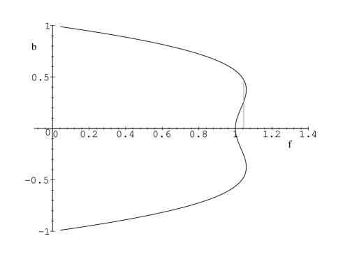
Figure 1: The order parameter $b$ in the $1/n$ expansion as a function of the coupling $f$ for $\omega=1$. There is a jump at $f_{c}(1)=1.046$ from a finite value to $b=0$ shown by the dotted line.

For $\omega<1$, the $b\to-b$ symmetry is broken and the local minimum with $b>0$ is the lowest. For $\omega$ only slightly less than 1, the situation is as in fig. 2. Here again, at some $f=f_{c}(\omega)$ the parameter $b$ undergoes a finite jump. There is, however, a critical value of $\omega=\omega_{c}\approx 0.985$ below which the “S-structure” in fig. 2 dissolves and there is only one extremal point for $b>0$ for all values of $f$. In the $\omega-f$ plane there is thus a first order transition line which starts at $(1,f_{c}(1))$, extends only a little way in the plane and ends at a critical point ${\rm C}=(\omega_{c},f_{c}(\omega_{c})\approx 1.075)$. At C the vector and tensor correlation lengths remain finite. The transition at C is, however, second order since the specific heat diverges. The cause of this in the leading order of the $1/n$ expansion can be traced back to a development of a singularity in the inverse propagator of the auxiliary fluctuating $t$-field at zero momentum at the critical point. The singularity in the $t-$ propagator seems to remain for higher orders as well. An infinite correlation length in the energy fluctuations does not contradict a finite correlation length in the vector and tensor channels; in particular, there is no conflict with correlation inequalities. These inequalities state that by increasing a ferromagnetic coupling the system becomes more ordered and the correlation between any spins increases. Although this assumption looks physically quite obvious, it has not been proven rigorously. The increase of the correlation function, however, implies the growing of a correlation length with increasing ferromagnetic coupling, only when the corresponding quantity has a vanishing expectation value.

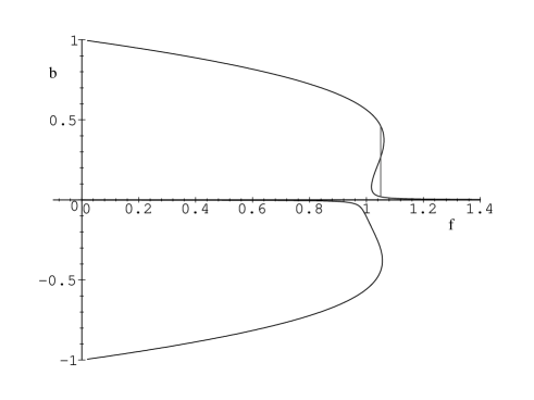
Figure 2: The order parameter $b$ as a function of $f$ for $\omega=0.999$. It still has a finite jump indicated by dotted line. At $\omega\geq\omega_{c}=0.985$ the S–shape dissolves thus the phase transition disappears.

Thus, a diverging vector (or tensor) correlation length at the endpoint C would contradict a finite correlation length for large (but finite) $\beta_{V}$ (asymptotic freedom) — on the other hand, a diverging specific heat at C is not excluded by these considerations. The above scenario disagrees with that of Magnoli and Ravanini  [7] who argue (based on correlation inequalities) that the second order phase transition at the point C is only an artifact of the $1/n$ approximation.

Caracciolo, Pelissetto and Sokal [16] also discuss the $\beta_{T}/N$, $\beta_{V}$ fixed, $N\to\infty$ limit. They obtain a result which is equivalent to eq. (26) above (although their interpretation is different from ours).

In conclusion, it is plausible that the phase diagram, also for finite $n$, is the “standard” one shown in fig. 3. There is a first order transition line starting at the point A of the $\beta_{T}$ axis. It ends at the point C where the specific heat becomes infinite, but the vector and tensor correlation lengths remain finite. In this figure we also indicate the Ising critical point B discussed in Section 3. The dotted line starting at point B is the critical line of the underlying Ising variable $\epsilon$. This criticality, however, does not show up in the correlation functions of the original variable ${\bf S}$.

Figure 3: The phase diagram for the mixed ${\rm RP}^{n-1}$ – ${\rm O}(n)$ model.

Acknowledgements. We thank Peter Hasenfratz and Erhard Seiler for useful discussions and Alan Sokal for a correspondence.

References

- [1] S. Caracciolo, R. G. Edwards, A. Pelissetto and A. D. Sokal, Nucl. Phys. B (Proc. Suppl.) 30 (1993) 815
- [2] S. Caracciolo, R. G. Edwards, A. Pelissetto and A. D. Sokal, Phys. Rev. Lett. 72 (1994) 179
-
[3]
J. Greensite and B. Lautrup, Phys. Rev. Lett. 47 (1981) 9;
I. G. Halliday and A. Schwimmer, Phys. Lett. 101B (1981) 327;
G. Bhanot, Phys. Lett. 108B (1982) 337;
G. Bhanot and R. Dashen, Phys. Lett. B113 (1982) 299,
for a recent work: T. Blum, C. DeTar, U. Heller, L. Kärkkäinen, K. Rummukainen and D. Toussaint, hep–lat/9412038, and references therein. - [4] J. Kosterlitz and D. Thouless, J. Phys. C6 (1973) 1181
- [5] U. Wolff, Phys. Rev. Lett. 62 (1989) 361; Nucl. Phys. B322 (1989) 759
- [6] H. Kunz and G. Zumbach, Phys. Rev. B46 (1992) 662
- [7] N. Magnoli and F. Ravanini, Z. Phys. C34 (1987) 43
- [8] H. Kunz and G. Zumbach, J. Phys. A22 (1989) L1043
- [9] S. Solomon, Phys. Lett. B100 (1981) 492
- [10] M. Fukugita, M. Kobayashi, M. Okawa, Y. Oyanagi and A. Ukawa, Phys. Lett. B109 (1982) 209
- [11] D. K. Sinclair, Nucl. Phys. B205[FS5] (1982) 173
- [12] A. Patrascioiu, E. Seiler, The Difference between the Abelian and Non–Abelian Models, Facts and Fancy, AZPH–TH/91–58 and MPI–Ph 91–88
- [13] E. Floratos and D. Petcher, Nucl. Phys. B252 (1985) 689
- [14] P. Hasenfratz and F. Niedermayer, Nucl. Phys. B414 (1994) 785
- [15] S. Caracciolo and A. Pelissetto, Nucl. Phys. B420 (1994) 141
- [16] S. Caracciolo, A. Pelissetto and A. D. Sokal, Nucl. Phys. B (Proc. Suppl.) 34 (1994) 683