BUTP–95/14
                                                                              COLO-HEP-361

The classically perfect fixed point action for SU(3) gauge theory

Thomas DeGrand, Anna Hasenfratz

Department of Physics

University of Colorado, Boulder CO 80309-390

Peter Hasenfratz, Ferenc Niedermayer

Institute for Theoretical Physics

University of Bern

Sidlerstrasse 5, CH-3012 Bern, Switzerland

March 2024

Abstract

In this paper (the first of a series) we describe the construction of fixed point actions for lattice $SU(3)$ pure gauge theory. Fixed point actions have scale invariant instanton solutions and the spectrum of their quadratic part is exact (they are classical perfect actions). We argue that the fixed point action is even 1–loop quantum perfect, i.e. in its physical predictions there are no $g^{2}a^{n}$ cut–off effects for any $n$. We discuss the construction of fixed point operators and present examples. The lowest order $q{\bar{q}}$ potential $V(\vec{r})$ obtained from the fixed point Polyakov loop correlator is free of any cut–off effects which go to zero as an inverse power of the distance $r$.

1 Introduction and summary

Using a discrete space–time lattice as an ultraviolet regulator for a quantum field theory also opens the way to many non–perturbative methods. At the same time however the lattice introduces various artifacts like rotational symmetry breaking. Cut–off independent continuum quantities are obtained in the limit of zero lattice spacing. Depending on the relevance of the lattice artifacts this limit can be reached on relatively coarse lattices or one might need lattices where the lattice spacing in physical units is extremely small. The main problem for numerical lattice calculations is the control of the finite lattice spacing effects.

The relevance of the lattice artifacts on the numerical results can strongly depend on the specific regularization or lattice action. Most numerical calculations to date of QCD use the Wilson plaquette action. This action is the simplest one which can be used but it has some undesirable properties. For example, asymptotic scaling sets in slowly and non–smoothly. Even more important is that the continuum limit is reached at lattice spacing less then 0.1 fm and, consequently, nowadays typical pure gauge or quenched calculations are done on spatial volumes $32^{3}$ or larger [1].

Two of us [2] suggested a radical solution, to use a perfect lattice action which is completely free of lattice artifacts. That such a perfect action exists follows from Wilson’s renormalization group theory [3]. The fixed point (FP) of a renormalization group (RG) transformation and the renormalized trajectory (RT) along which the action runs under repeated RG transformations form a perfect quantum action. The FP action itself reproduces all the important properties of the continuum classical action (it is a classical perfect action). Although at finite coupling values the FP action is not “quantum perfect” it is expected to be a very good first approximation. This program was successfully carried out for the 2–dimensional non–linear $\sigma$ model. An action parametrized by about 20 parameters was found that showed no finite lattice spacing effects even at correlation length $\xi\sim 3$ lattice spacings. The computational overhead to simulate this action (about a factor of three relative to the nearest neighbor action) is negligible compared to the gain obtained by the great reduction of lattice artifacts.

Figure 1: The quantity $rV(r)$ constructed from the correlators of the FP Polyakov loops and using the FP action. Note that $1/4\pi=.0796$.

Figure 2: The quantity $rV(r)$ constructed for the Symanzik action.

Figure 3: The quantity $rV(r)$ constructed for the Wilson action.

In this and a follow up paper [5] we report on a similar project for the 4–dimensional pure gauge SU(3) theory. We construct FP actions and FP operators and investigate their properties. In this first paper the basic equations are presented and the properties of the FP action and operators are investigated on fields with small fluctuations. The methods used are mostly analytic. In the second paper we turn to the problem of using the FP action in numerical simulations on coarse lattices. A simple parametrization is derived and the scaling properties of the action are studied by measuring torelon masses and the potential.

In the present paper we consider two different type of RG transformations. Both transformations contain free parameters which are used to make the FP action as short ranged as possible. For any practical application this is a basic requirement. The FP action is defined by a classical saddle point equation. It follows from this equation that the FP action has exact stable instantons. The value of the action for the instantons is $8\pi^{2}$ independently of the size of the instanton (scale invariance). The FP equation can be solved analytically on fields with small fluctuations by expanding in powers of the vector potentials. The quadratic part of the FP action describes massless gluons with an exact relativistic spectrum: $E=|\vec{p}|$, $p_{i}\in(-\infty,\infty)$. This is to be contrasted with that of the Wilson action where this dispersion relation is valid only for $|\vec{q}|\ll 1$ and, in addition, the spectrum is restricted to the Brillouin zone $|q_{i}|\leq\pi$. For small $|\vec{q}|$ the Symanzik tree level improved action [6], [7] performs better, but then, in the middle of the Brillouin zone it breaks down completely producing complex energies.

An exciting question is how the FP action performs in 1–loop perturbation theory. We present a formal RG argument that the physical predictions are free of cut–off effects O($a^{n}$) and O($g^{2}a^{n}$) for any $n$ provided the size of the system is larger then the range of the action. Is therefore the classical perfect action automatically 1–loop quantum perfect? Our RG arguments are formal, not rigorous. The statement is supported further by a detailed 1–loop calculation in the non–linear $\sigma$ model [8] where the cut–off effects of the mass gap are studied in a finite box of size $L$. The power like decaying cut–off effects $(a/L)^{n}$ were found several orders of magnitude smaller (and consistent with zero within the errors of the calculation) than those in the standard or in the tree level improved Symanzik model.

We need not only perfect actions but perfect Polyakov, or Wilson loops, currents, etc. as well. As a first step we discuss here how to construct FP operators. We derive the explicit form of the FP Polyakov loop on fields with small fluctuations and obtain the corresponding tree level $q\bar{q}$ potential $V(\vec{r})$. We show that $V(\vec{r})$ is free of any cut–off effects which decay as a power $r^{-k}$ for large $r$. This property is to be contrasted with that of the standard and Symanzik action. In the latter case only the leading O($a^{2}$) distortion is canceled. The situation is illustrated in Figs. 1, 2 and 3.

Kerres, Mack, and Palma[9] have recently described the construction of a perfect action for scalar electrodynamics in four dimensions and at finite temperature. Some of the basic ideas of [9] overlap with those introduced in [2] and in the present work.

The outline of the paper is as follows. In Section 2 the two different RG transformations we considered are defined. In Section 3 the FP equation is derived and the statement about classical solutions of the FP action is discussed briefly. In Sections 4 and 5 the FP action is constructed at the quadratic level and the spectrum is studied. In Section 6 the main steps leading to the cubic terms of the action are presented. Section 7 deals with the question of whether the FP action is 1–loop quantum perfect. The problem of FP operators is discussed in Section 8.

2 The RG transformation

Consider an SU(N) gauge theory defined on a hypercubic lattice. The partition function is

$$Z=\int DUe^{-\beta S(U)},$$ (1)

where $\beta S(U)$ is some lattice representation of the continuum action. It is a function of the products of link variables $U_{\mu}(n)=e^{iA_{\mu}(n)}\in$SU(N) along arbitrary closed loops. The normalization is fixed such that on smooth configurations the action takes the standard continuum form

$$\beta S(U)\rightarrow{1\over{2g^{2}}}\int d^{4}xTr\left(F_{\mu\nu}F_{\mu\nu}\right),$$ (2)

where

$$\beta={2N\over g^{2}}.$$ (3)

Let us denote the couplings of $\beta S(U)$ by $\beta$, $c_{2},c_{3},\ldots$. The action can be represented by a point in this infinite dimensional coupling constant space as shown in fig. 4.

Figure 4: Schematic flow diagram for asymptotically free gauge theories.

Under repeated real space renormalization group transformations the action moves in this multidimensional parameter space. We shall consider RG transformations with a scale factor of 2. The blocked link variable $V_{\mu}(n_{B})\in$SU(N), which lives on the coarse lattice with lattice unit $a^{\prime}=2a$, is coupled to a local average of the original link variables. The new action is defined as

$${\rm e}^{-\beta^{\prime}S^{\prime}(V)}=\int DU\exp\left\{-\beta\left(S(U)+T(U,V)\right)\right\},$$ (4)

where the blocking kernel $T(U,V)$ is taken in the form

$$T(U,V)=\sum_{n_{B},\mu}\left\{-{\kappa\over N}{\rm ReTr}\left(V_{\mu}(n_{B})Q^{\dagger}_{\mu}(n_{B})\right)+{\cal N}\left(Q_{\mu}(n_{B})\right)\right\}.$$ (5)

The $N\times N$ complex matrix $Q_{\mu}(n_{B})$ is an average of the fine link variables in the neighbourhood of the coarse link $l_{B}=(n_{B},\mu)$. Its explicit form will be specified later. The last term in Eq. (5) assures that the partition function remains invariant under the RG transformation,

$${\rm e}^{\beta{\cal N}(Q)}=\int dW\exp\left\{\beta{\kappa\over N}{\rm ReTr}(WQ^{\dagger})\right\},~{}~{}~{}W\in{\rm SU(N)}\,.$$ (6)

The parameter $\kappa$ is free and will be used for optimization as in [2]. We require the averaging procedure to be gauge invariant

$$T\left(U^{g},V^{g}\right)=T(U,V),$$ (7)

where $U^{g}$ and $V^{g}$ are gauge transformed configurations on the fine and coarse lattice, respectively. This property, together with the gauge symmetry of the action $S(U)$, assures that $S^{\prime}(V)$ is also gauge invariant.

In this paper we consider two different block transformations which will be referred to as type I and type II, respectively. The first transformation we used is a modified version of the Swendsen transformation [10] shown in fig. 5 where $c$, the relative weight of the staples vs. the central link, is a tunable parameter:

Figure 5: The renormalization group transformation of type I.

$$Q_{\mu}(n_{B})=(1-6c)U_{\mu}(n)U_{\mu}(n+\mu)+~{}~{}~{}~{}~{}~{}~{}~{}~{}$$

$$c\sum_{\nu\neq\mu}\left[U_{\nu}(n)U_{\mu}(n+\nu)U_{\mu}(n+\mu+\nu)U^{\dagger}_{\nu}(n+2\mu)+\right.$$ (8)

$$\left.U_{\nu}^{\dagger}(n-\nu)U_{\mu}(n-\nu)U_{\mu}(n+\mu-\nu)U_{\nu}(n+2\mu-\nu)\right].$$

The second transformation uses smearing to create fuzzy links. The matrix $Q_{\mu}(n_{B})$ is the product of the two fuzzy link variables obtained after two smearing steps. The construction is shown in fig. 6.

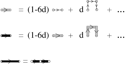
Figure 6: The renormalization group transformation of type II.

Here $c$ and $d$ are tunable parameters. With $c=1/7$ the transformation Eq. (8) is identical to the one used in the $\beta$ function calculations earlier [10].

It is expected that these RG transformations have a fixed point (FP) on the $\beta=\infty$ critical surface. The FP has one marginally relevant and infinitely many irrelevant directions. The trajectory which leaves the FP along the marginal direction is the renormalized trajectory (RT).

As it was argued in [2] the FP and the RT describe perfect actions. There are no lattice artifacts along the RT. For reasons discussed in the Introduction and later, we shall refer to the FP action $\beta S^{FP}(U)$ as the classical perfect action. This is the action we shall consider in this work. Although this action does not lie on the RT at finite $\beta$ values, it has amazingly nice properties at large $\beta$ and shows no, or tiny, cut–off effects even on very coarse configurations.

3 The fixed point equation

On the critical surface $\beta\to\infty$ Eq. (4) reduces to a saddle point problem giving

$$S^{FP}(V)=\min_{\{U\}}\left(S^{FP}(U)+T(U,V)\right),$$ (9)

where $S^{FP}$ is the FP action. For a given coarse configuration $\{V\}$ there are infinitely many minimizing $\{U\}$ configurations which differ by gauge transformations leaving the averages $Q_{\mu}(n_{B})$ invariant. The value of the FP action $S^{FP}(V)$ is not influenced by this freedom, however.

Using Eqs. (5,6) the saddle point equation can be written as

$$S^{FP}(V)=\min_{\{U\}}\left\{S^{FP}(U)-{\kappa\over N}\sum_{n_{B},\mu}\left[{\rm ReTr}\left(V_{\mu}(n_{B})Q_{\mu}^{\dagger}(n_{B})\right)-f\left(Q_{\mu}(n_{B})\right)\right]\right\},$$ (10)

where

$$f(Q)=\max_{W}\left\{{\rm ReTr}(WQ^{\dagger})\right\},~{}~{}~{}~{}W\in{\rm SU}(N).$$ (11)

This equation has a very similar structure to the one in the $d=2$ non–linear $\sigma$–model [2] and its implications for the classical solutions of $S^{FP}$ are the same: if the configuration $\{V\}$ satisfies the FP classical equations and is a local minimum of $S^{FP}(V)$ then the configuration $\{U(V)\}$ on the finer lattice minimizing the r.h.s.. of Eq. (10) satisfies the FP equations as well. In addition, the value of the action remains unchanged, $S^{FP}(V)=S^{FP}(U(V))$.

Since the proof goes along the same lines as in the $d=2$ $\sigma$–model [2], we can be brief here. If $\{V\}$ is a solution of the classical equations of motion $\delta S^{FP}/\delta V=0$, then Eq. (10) implies that on the minimizing configuration $\{U(V)\}$ the expression in square brackets in Eq. (10) takes its maximum value, i.e. zero. Then it follows that

$$\left.{\delta S^{FP}(U)\over\delta U}\right|_{U=U(V)}=0,$$ (12)

and $S^{FP}(V)=S^{FP}(U(V))$.

According to this result the FP action has exact scale invariant instanton solutions with action $=8\pi^{2}$ as in the continuum theory. This property allows one to define a correct topological charge on the lattice [11]. In this paper, however, we will not follow this problem further.

4 The FP action at the quadratic level

The FP equation Eq. (10) is valid for any configuration $\{V\}$, be it smooth or rough. It is a highly non–trivial equation. On $\{V\}$ configurations with small fluctuations, however Eq. (10) can be expanded in powers of the vector potentials and studied analytically.

On the quadratic level we can write.

$$2NS(U)=\sum_{n,r}\rho_{\mu\nu}(r){\rm Tr}\left(A_{\mu}(n+r)A_{\nu}(n)\right)+{\rm O}\left(A^{3}\right)$$ (13)

$${\phantom{2NS(U)}}={1\over V}\sum_{k}\tilde{\rho}_{\mu\nu}(k){\rm Tr}\left(\tilde{A}_{\mu}(-k)\tilde{A}_{\nu}(k)\right)+{\rm O}\left(\tilde{A}^{3}\right),$$

where $\rho_{\mu\nu}(r)$ (in momentum space $\tilde{\rho}_{\mu\nu}(k)$) are the quadratic couplings to be determined. Gauge symmetry and the normalization condition Eq. (2) give the constraints

$$\widehat{k}_{\mu}^{*}\rho_{\mu\nu}(k)=0,$$ (14)

$$\rho_{\mu\nu}(k)\to k^{2}\delta_{\mu\nu}-k_{\mu}k_{\nu}~{}~{}~{}{\rm for~{}}k\to 0,$$

where we introduced the notation $\widehat{k}_{\mu}={\rm e}^{ik_{\mu}}-1$. For both RG transformations (fig. 5 and fig. 6) $Q_{\mu}(n_{B})$ is a sum over products of $U$ matrices along paths connecting the points $n$ and $n+2\widehat{\mu}$. It is easy to show that

$${\rm ReTr}\left(V_{\mu}(n_{B})Q_{\mu}^{\dagger}(n_{B})\right)-f(Q_{\mu}(n_{B}))=-{1\over 2}{\rm Tr}\left(\Gamma_{\mu}(n_{B})-B_{\mu}(n_{B})\right)^{2}+{\rm O}\left({\rm cubic}\right),$$ (15)

where

$$\Gamma_{\mu}(n_{B})=\sum_{r,\nu}\omega_{\mu\nu}(2n_{B}-r)A_{\nu}(r)\,.$$ (16)

In Eq. (16) the tensor $\omega_{\mu\nu}$ is fixed by the form of the RG transformation kernel in fig. 5 and fig. 6:

$$\omega_{\mu\nu}(k)=\left(1+{\rm e}^{ik_{\mu}}\right)\left[\delta_{\mu\nu}\left(1-c(\widehat{k}\widehat{k}^{*})\right)+c\widehat{k}_{\mu}\widehat{k}_{\nu}^{*}\right],~{}~{}~{}{\rm type~{}I},$$ (17)

$$\omega_{\mu\nu}(k)=\left(1+{\rm e}^{ik_{\mu}}\right)\left[\delta_{\mu\nu}\left(1-d(\widehat{k}\widehat{k}^{*})\right)^{2}+d\left(2-d(\widehat{k}\widehat{k}^{*})\right)\widehat{k}_{\mu}\widehat{k}_{\nu}^{*}\right],~{}~{}{\rm type~{}II}.$$ (18)

At the quadratic level the recursion relation has the form

$${1\over V_{B}}\sum_{k_{B}}\rho^{\prime}_{\mu\nu}(k_{B}){\rm Tr}\left(B_{\mu}(-k_{B})B_{\nu}(k_{B})\right)=$$

$$\min_{\{A\}}\left\{{1\over V}\sum_{k}\rho_{\mu\nu}(k){\rm Tr}\left(A_{\mu}(-k)A_{\nu}(k)\right)\right.+$$ (19)

$$\left.\kappa{1\over V_{B}}\sum_{k_{B}}{\rm Tr}\left[\left(\Gamma_{\mu}(-k_{B})-B_{\mu}(-k_{B})\right)\left(\Gamma_{\mu}(k_{B})-B_{\mu}(k_{B})\right)\right]\right\}\,,$$

where $V_{B}={1\over 16}V$ is the volume of the blocked lattice. To proceed further we have to introduce a temporary gauge fixing to get rid of the remaining gauge freedom at the sites of the fine lattice not representing a site on the coarse lattice. One obtains then from Eq. (19) a recursion relation for the inverse of $\rho$:

$$D^{\prime}_{\mu\nu}(q_{B})={1\over 16}\sum_{l=0}^{1}\left[\omega({q_{B}\over 2}+\pi l)D({q_{B}\over 2}+\pi l)\omega^{\dagger}({q_{B}\over 2}+\pi l)\right]_{\mu\nu}+{1\over\kappa}\delta_{\mu\nu}\,,$$ (20)

where $l=(l_{0},l_{1},l_{2},l_{3})$ is an integer vector, the summation goes over $l_{\mu}=0,1$ and

$$D_{\mu\nu}(q_{B})=\left(\rho^{-1}(q_{B})\right)_{\mu\nu}\,.$$ (21)

A way to find the FP solution of Eq. (20) is to start from a $D^{(0)}_{\mu\nu}(q)$ with some gauge fixing parameter $\alpha$

$$D^{(0)}_{\mu\nu}(q)={1\over(\widehat{q}\widehat{q}^{*})}\delta_{\mu\nu}+\alpha{\widehat{q}_{\mu}\widehat{q}^{*}_{\nu}\over(\widehat{q}\widehat{q}^{*})^{2}}\,,$$ (22)

and iterate Eq. (20) to the FP solution $D^{FP}_{\mu\nu}$. The inverse of $D^{FP}_{\mu\nu}$ has a smooth $\alpha\to\infty$ limit which corresponds to removing the gauge fixing. The resulting $\rho^{FP}_{\mu\nu}(k)$ is transverse and satisfies Eq. (14).

The program sketched above is not completely trivial. The main steps and some intermediate results are collected in Appendix A.

The fixed point $\rho^{FP}_{\mu\nu}$ depends on the parameters of the RG transformation $(\kappa,c)$, or $(\kappa,d)$ for the kernels of type I and type II, respectively. Although none of the theoretical properties of the FP action depend on these parameters, the range of $\rho^{FP}_{\mu\nu}(r)$ (the range of the interaction) changes significantly as these parameters are varied. It is vital in applications that the interaction is short ranged. Using this requirement we found that the following parameter values are close to optimal:

$$\kappa=12.0,~{}~{}~{} c=0.12,~{}~{}~{}{\rm type~{}I}\,,$$ (23)

$$\kappa=10.5,~{}~{}~{} d=0.077,~{}~{}~{}{\rm type~{}II}\,.$$

Using these values the significantly non–zero couplings lie in the unit hypercube and $\rho^{FP}_{\mu\nu}(r)$ goes rapidly to zero with the distance. The decrease seems to be as fast as $\approx\exp(-3r)$. In Table 1 and 2 we collected some of the elements of $\rho^{FP}_{\mu\nu}(r)$ for the RG transformation of type I and II, respectively. Using these tables, plus the cyclic permutation of the coordinates and the reflection properties of $\rho_{\mu\nu}(r)$ (Appendix B), further elements can be obtained.

$r$	$\rho_{00}(r)$	$r$	$\rho_{10}(r)$
0 0 0 1	-0.6718	0 0 0 0	-0.8007
0 0 0 2	0.02420	0 0 0 1	-0.03100
0 0 0 3	-0.00422	0 0 0 2	-0.00170
1 0 0 0	-0.05951	0 1 0 0	0.01129
0 0 1 1	-0.04281	0 1 0 1	-0.00208
1 0 0 1	0.01614	1 0 1 1	0.00880
0 1 1 1	-0.02724	2 1 0 0	-0.00387

Table 1: Some of the elements of $\rho_{00}(r)$ and $\rho_{10}(r)$ for the RG transformation of type I.

$r$	$\rho_{00}(r)$	$r$	$\rho_{10}(r)$
0 0 0 1	-0.5872	0 0 0 0	-0.7777
0 0 0 2	0.00769	0 0 0 1	-0.04813
0 0 0 3	-0.00035	0 0 0 2	-0.00081
1 0 0 0	0.00467	0 1 0 0	-0.00102
0 0 1 1	-0.07964	0 1 0 1	-0.00063
1 0 0 1	-0.00298	1 0 1 1	0.00804
0 1 1 1	-0.02490	2 1 0 0	-0.00571

Table 2: Some of the elements of $\rho_{00}(r)$ and $\rho_{10}(r)$ for the RG transformation of type II.

5 The spectrum of the quadratic FP action

Although the quadratic FP action Eq. (13) lives on the lattice, it describes transverse massless gluons with an exact relativistic spectrum $E(\vec{k})=|\vec{k}|$, $k_{i}\in(-\infty,\infty)$. This follows from the fact that the FP action represents in fact an infinitely fine lattice, i.e. the continuum. A similar property has been demonstrated earlier for the $d=2$ non–linear $\sigma$–model [2] where this statement follows trivially from an explicit closed representation of the FP propagator. This property is to be contrasted with that of the standard or Symanzik improved actions where the spectrum is distorted by O($a^{2}$), or O($a^{4}$) cut–off effects, respectively. A distorted spectrum implies distorted thermodynamics. Large cut–off effects are seen in the free energy at high temperatures both in perturbation theory and in numerical simulations [12].

The spectrum is determined by the singularities of the propagator $D_{\mu\nu}(q)$. Consider this propagator after $n$ RG steps as given by Eq. (A7) in Appendix A. The $\sim\delta_{\mu\nu}$ part of $D^{(0)}_{\mu\nu}(q)$ gives for large $n$ the term

$$\left[\Omega^{(n)}\left({q+2\pi l\over 2^{n}}\right)\Omega^{(n)\dagger}\left({q+2\pi l\over 2^{n}}\right)\right]_{\mu\nu}{1\over(q+2\pi l)^{2}}\,.$$ (24)

The tensor $\Omega^{(n)}$ is a smearing function which builds up the blocked link after $n$ RG steps out of the original link variables. This is a local function in configuration space whose Fourier transform is smooth, $\Omega^{(n)}_{\mu\nu}(q=0)=\delta_{\mu\nu}$. Eq. (24) has a pole at $k_{0}=\pm i|\vec{k}|$, where $k=q+2\pi l$. For any given $\vec{q}$, $q_{i}\in(0,2\pi)$ the summation over $l$ gives a tower of poles in $D_{\mu\nu}(q)$ which reproduce the full relativistic spectrum of the continuum theory.

The terms proportional to $1/\kappa$ in Eq. (A7) are constructed out of $\Omega_{\mu\nu}$ and do not change this conclusion. Similarly, the part of $D_{\mu\nu}$ proportional to the gauge fixing parameter $\alpha$ is removed at the end and does not influence the form of $\rho^{FP}(q)$ (cf. Appendix A).

In Fig. 7 we compare the spectrum of the quadratic parts of the Wilson, Symanzik improved and FP actions. Our parameterization of the Symanzik actions follows the notation of Weisz [7]. For the Wilson and Symanzik actions the momentum in Fig. 7 is restricted to lie along one of the lattice axes. The energy-momentum relation for the action labelled S1 becomes complex at large $k$; the dotted line shows its real part.

Figure 7: The spectrum of the quadratic part for the Wilson action (W), the Symanzik improved action for two different choices of the coefficients: S1: $c_{1}=-1/12$, $c_{2}+c_{3}=0$, S2: $c_{1}=0$, $c_{2}+c_{3}=1/12$, and the FP action.

6 The connecting tensor $Z_{\mu\nu}(n)$ and the FP action at the cubic level

In an SU(N) non Abelian theory gauge symmetry implies the presence of terms in the action which are cubic in the vector potentials. Gauge symmetry alone, however, does not fix the cubic part of the action. There are combinations of Wilson loops whose contribution to the quadratic part is zero while to the cubic part is not. The cubic part of the FP action is, however, uniquely given by the FP equation Eq. (10).

One expands Eq. (10) up to terms cubic in the coarse ($B_{\mu}$) and fine ($A_{\mu}$) vector potentials. The action is written in the form

$$2N\cdot S(U)={1\over 2}\sum_{n,r}\rho_{\mu\nu}(r)A^{a}_{\mu}(n+r)A^{a}_{\nu}(n)+$$ (25)

$${1\over 12}f^{abc}\sum_{n,r_{1},r_{2}}c_{\mu\nu\rho}(r_{1},r_{2})A^{a}_{\mu}(n+r_{1})A^{b}_{\nu}(n+r_{2})A^{c}_{\rho}(n)+{\rm O}\left(A^{4}\right),$$

where in terms of the SU(N) generators,

$$\left[T^{a},T^{b}\right]=if^{abc}T^{c},~{}~{}~{}{\rm Tr}T^{a}T^{b}={1\over 2}\delta_{ab}\,.$$ (26)

The terms proportional to $\kappa$ in Eq. (10) are expanded to cubic order as well. The quadratic and cubic coupling constant tensors $\rho_{\mu\nu}(r)$ and $c_{\mu\nu\rho}(r_{1},r_{2})$ are determined then by the FP condition Eq. (10).

After introducing a gauge fixing term in the action and solving the quadratic problem one obtains the minimizing fine vector potentials as a function of the coarse fields (Appendix A). In configuration space this relation can be written in the form

$$A^{a}_{\mu}(n)=\sum_{n^{\prime}_{B}}Z_{\mu\rho}(n-2n^{\prime}_{B})B^{a}_{\rho}(n^{\prime}_{B}).$$ (27)

Since the minimizing configuration is fixed only up to gauge transformations (cf. Section 2), the very definition of the relation in Eq. (27) requires gauge fixing. We used the type of gauge fixing given in Eq. (22) and defined the connecting tensor $Z_{\mu\nu}$ in the $\alpha\to\infty$ limit. Using eqs. (A5),(A6) one obtains

$$Z_{\mu\rho}(n-2n^{\prime}_{B})=\lim_{{\alpha\to\infty\atop n\to\infty}}{1\over V_{B}}\sum_{k_{B}}{1\over 16}\sum_{l=0}^{1}{\rm e}^{i({1\over 2}k_{B}+\pi l)(n-2n^{\prime}_{B})}\times$$ (28)

$$\left[D^{(n)}({k_{B}\over 2}+\pi l)\omega^{\dagger}({k_{B}\over 2}+\pi l)\left(D^{(n+1)}(k_{B})\right)^{-1}\right]_{\mu\rho}$$

Note that sites on the fine lattice can be labeled as $n=2n_{B}+m$, $m_{\mu}=0,1$. In Fourier space one obtains

$$Z_{\mu\rho}(q)=\left[D^{(n)}(q)\omega^{\dagger}(q)\left(D^{(n+1)}(2q)\right)^{-1}\right]_{\mu\rho}\,.$$

The tensor $Z_{\mu\nu}$ is an important quantity which enters not only the cubic calculation, but also the construction of the fixed point operators, like the FP Polyakov loop (cf. section 8). The connecting function decays rapidly with distance; the minimizing configuration is determined locally by the coarse vector potential $B_{\mu}$. In Table 3 a few leading elements of $Z_{00}$ and $Z_{10}$ are collected for the two different block transformations. A permutation of the coordinates and the (somewhat unusual) reflection properties of $Z_{\mu\nu}$ (Appendix B) help one to find its value for further related $\mu,\nu$ and $n$ values.

$n$	$Z_{00}^{I}$	$Z_{00}^{II}$	$n$	$Z_{10}^{I}$	$Z_{10}^{II}$
0 0 0 0	0.4031	0.4442	0 0 0 0	0.0878	0.0751
0 1 0 0	0.1756	0.1413	0 1 0 0	-0.0408	-0.0475
0 0 1 1	0.0610	0.0623	2 1 0 1	0.0226	0.0153
-1 1 0 0	0.0514	0.0526	3 1 0 0	0.0217	0.0148
0 1 1 1	0.0339	0.0345

Table 3: Some of the elements of the tensor $Z_{\mu\nu}$ which gives the minimizing configuration in terms of the coarse vector potential for the block transformation type I and type II.

The minimizing vector potential is given by Eq. (27) only in the quadratic approximation. Nevertheless, this expression can also be used when we need the minimum in Eq. (10) up to cubic order. The error made is only quartic. This way all the cubic terms in Eq. (10) will be expressed in terms of the coarse fields $B^{a}_{\mu}$ and one obtains the following recursion relation for the cubic coefficients

$$c^{\prime}_{\mu\nu\rho}(r_{1},r_{2})=\kappa H_{\mu\nu\rho}(r_{1},r_{2})+$$ (29)

$$\sum_{n,n^{\prime},n^{\prime\prime}}c_{\mu^{\prime}\nu^{\prime}\rho^{\prime}}(n^{\prime}-n,n^{\prime\prime}-n)Z_{\mu^{\prime}\mu}(n^{\prime}-r_{1})Z_{\nu^{\prime}\nu}(n^{\prime\prime}-r_{2})Z_{\rho^{\prime}\rho}(n)$$

where $H_{\mu\nu\rho}$ comes from expanding Eq. (15) up to cubic order. The form of $H_{\mu\nu\rho}$ depends on the block transformation. We discuss here neither the explicit form of this tensor nor the details of solving Eq. (29) for the FP cubic couplings. In Table 4 we give some of the largest elements of $c_{\mu\nu\rho}(r_{1},r_{2})$ for the block transformation of type I (for type II we have not yet studied the cubic problem). Other related elements can be obtained by using the symmetry properties of the cubic coupling tensor.

We shall return to the cubic couplings in paper II when we discuss the general problem of the parametrization of the FP action in terms of loops.

$r_{1}$	$r_{2}$	$c_{000}(r_{1},r_{2})$
-2  0  0  0	-1  0  0  0	-0.019
-1 -1  0  0	-1  0  0  0	-0.012
-1 -2  0  0	-1 -1  0  0	-0.005
-2 -1  0  0	-1 -1  0  0	0.002
$r_{1}$	$r_{2}$	$c_{100}(r_{1},r_{2})$
0 -1  0  0	0 -1  0  0	-0.598
0 -1 -1  0	0  0 -1  0	0.027
0 -1  0  0	-1 -1  0  0	-0.027
0 -2  0  0	0 -2  0  0	0.025
$r_{1}$	$r_{2}$	$c_{210}(r_{1},r_{2})$
0 -1 -1  0	0 -1  0  0	-0.062
0 -1 -1 -1	0 -1  0 -1	-0.007
-1  0 -1  0	0 -1 -1  0	-0.004
0 -1 -1  0	0 -1  0 -1	-0.004

Table 4: Some of the largest cubic couplings for the type I RG transformation.

7 Cut–off independence of physical predictions of the FP action in 1–loop perturbation theory

As discussed in Section 4, in leading order (tree level) perturbation theory the FP action gives cut–off independent physical predictions. Formal RG considerations suggest that the renormalized trajectory coincides with the FP action even at 1–loop level. That would imply that the predictions using the FP action are free of lattice artifacts even in 1–loop perturbation theory. Said differently: the predictions of the classical perfect action (FP action) contain no O$\left(a^{n}\right)$ nor O$\left(g^{2}a^{n}\ln a,g^{2}a^{n}\right)$ corrections for any $n\geq 1.$

This is a strong statement which, unfortunately, we are not able to support by a rigorous proof. We shall present the formal RG arguments for an infinite system which show that the only effect of the perturbative $g^{2}$ corrections is to make the marginal operator $S^{FP}(U)$ weakly relevant, i.e. the coupling $\beta=2N/g^{2}$ begins to move, but the form of the action on the renormalized trajectory remains unchanged in this order:

$$\beta S^{FP}(U)\longrightarrow\beta^{\prime}S^{FP}(V)\,,$$ (30)

under a RG transformation, to 1–loop level. Here $\beta^{\prime}=\beta-\Delta\beta$, where $\Delta\beta$ is fixed by the first universal coefficient of the $\beta$–function. (For a scale 2 block transformation $\Delta\beta=0.579$ in SU(3).) An equation analogous to Eq. (30) occurred in ref. [13] where Wilson referred to formal RG arguments which were not, however, presented there.

Stronger arguments come from an explicit perturbative calculation with the FP action of the non–linear $\sigma$–model in $d=2$ [8]. In ref. [8] the mass gap $m(L)$ was calculated in a finite periodic box of size $L$. The prediction of the standard action is contaminated by power like cut–off effects $(a^{2}/L^{2})^{n},n=1,2,...$. These type of cut–off effects are eliminated when the FP action is used. More precisely, in the actual calculation they are reduced to the level of the numerical precision. For example, in the range of $L\sim 5~{}-~{}10$ the cut–off effect is reduced by 5 orders of magnitude relative to that of the standard action. On the other hand, there exists a small non-power like cut-off effect, which is seen at $L=2$, and goes to zero so rapidly that for $L>3$ it disappears in the numerical errors. This behaviour can be associated with the small, but finite, range of the FP action.

Let us present now the formal RG arguments. Consider a theory which has one marginal operator $R_{1}(U)$ and many irrelevant operators $R_{n}(U)$, $n=2,\dots$. The action is

$$S=R_{1}(U)+c_{2}R_{2}(U)+\dots$$ (31)

and the Boltzmann factor is $e^{-\beta S(U)}$, $\beta=2N/g^{2}$ for SU(N) gauge theories, while $R_{1}(U)$ is the FP action $S^{FP}(U)$ in our earlier notations. Under an RG transformation

$$S \longrightarrow S^{\prime}=R_{1}(V)+c_{2}^{\prime}R_{2}(V)+\dots$$

$$\beta \longrightarrow \beta^{\prime}.$$ (32)

If the theory is asymptotically free the critical surface is at $g=0$. A linearized scale $s$ transformation at the fixed point is described by

$$g \rightarrow g$$ (33)

$$c_{j} \rightarrow \lambda_{j}c_{j}$$ (34)

where $\lambda_{j}=s^{k_{j}}<1$ since the $R_{j}$’s are irrelevant. As the fixed point is at $g=0$, the exponents $k_{j}$ are given by dimensional analysis.

Now we consider general RG flows near the FP. For simplicity we introduce the notation $c_{1}=g^{2}$.

$$c_{1}^{\prime} = c_{1}+\alpha_{ij}^{(1)}c_{i}c_{j}+O(c^{3})$$ (35)

$$c_{k}^{\prime} = \lambda_{k}c_{k}+\alpha_{ij}^{(k)}c_{i}c_{j}+O(c^{3}).$$ (36)

If we start with the action

$$S^{FP}=R_{1},$$ (37)

$c_{1}$ small, $c_{2}=c_{3}=...=0$, i. e. the classical fixed point action, then after one RG step

$$c_{1}^{\prime} = c_{1}+\alpha_{11}^{(1)}c_{1}^{2}+O(c^{3})$$ (38)

$$c_{k}^{\prime} = \alpha_{11}^{(k)}c_{1}^{2}+O(c^{3}),$$ (39)

or

$${1\over g^{2}}S^{FP}\rightarrow{1\over{g^{2}+\alpha_{11}^{(1)}g^{4}}}(S^{FP}+\alpha_{11}^{(2)}g^{4}R_{2}+\alpha_{11}^{(3)}g^{4}R_{3}+\dots)$$ (40)

Noticing that the prefactor can be written

$${1\over{g^{2}+\alpha_{11}^{(1)}g^{4}}}={1\over{g^{2}}}-\alpha_{11}^{(1)}+O(g^{2})$$ (41)

we see that to leading order in $g^{2}$ the effect of the RG transformation is only to shift the coupling

$$\beta S^{FP}\rightarrow\left(\beta-\alpha_{11}^{(1)}\right)\left(S^{FP}+{{\alpha_{11}^{(2)}}\over{\beta^{2}}}R_{2}+\dots\right)\,,$$ (42)

and that the action itself is changed only in order $g^{4}$. The shift in $\beta$, $\alpha^{(1)}_{11}$, is equal to $\Delta\beta$ introduced earlier.

8 Fixed point operators

The action on the renormalized trajectory is perfect — it has only physical excitations. In a Green’s function only physical states come in as intermediate states independent of the operator used. In spite of that Green’s functions (of fields, currents, etc.) show cut–off effects in general. Consider, for example a free scalar field. As Eq. (21) of ref. [2] shows the perfect action on the lattice is described by a lattice field which is the integral of the continuum field over a hypercube. Therefore, the two-point function of the lattice field in the perfect action is equal to the two-point function of the continuum field averaged over the hypercubes around the the two lattice points in question. This averaging brings in a trivial rotation symmetry breaking. The two-point function of the field in the perfect action is not rotationally invariant, although only physical states propagate.

A more interesting example is the static quark creation operator represented conventionally by a Polyakov loop (or by one of the lines of an elongated Wilson loop) The two-point function gives the quark-antiquark potential. The potential measured with the Wilson action at distances $a$ , $\sqrt{2}a$ ,$\sqrt{3}a$, $2a,\dots$ is non-smooth even at large beta values — it reflects the hypercubic lattice structure rather than physics. This is unfortunate since in numerical simulations these points lie in the physically interesting region. In addition, these are the points with the smallest statistical errors. One expects that simple Polyakov loops constructed in terms of the fields of the perfect action behave better, since the cut–off effects due to the distorted spectrum are eliminated. However, in order to get rid of the remaining cut–off effects we have to modify the operator itself.

The first step in this direction is to construct FP operators along the lines by which the FP action was constructed. In Section 8.1 we use the example of the Polyakov loop to illustrate how to obtain the corresponding classical FP equation. In Section 8.2 we turn to the simple example of a scalar field theory in $d=2$ and construct the FP field on the lattice. We show that the two–point function of the FP field is free of any cut–off effects of order $(a/r)^{n}$. On the other hand, the FP field two–point function differs from the exact continuum propagator $-(2\pi)^{-1}\ln r+{\rm const}$ by terms which decrease exponentially with $r$. In Section 8.3 we solve the FP equation for the Polyakov loop in quadratic approximation in the vector potentials, calculate the corresponding $q\bar{q}$ potential (which is $-(4\pi r)^{-1}$ in the continuum limit) and compare it with that of the standard and Symanzik improved actions.

8.1 The FP Polyakov loop

Consider the correlator $\left.\langle L(\vec{n})L^{\dagger}(\vec{m})\rangle\right|_{S^{FP}},$ where $L(\vec{n})$ is a Polyakov loop running in the temporal direction at the spatial point $\vec{n}=(n_{1},n_{2},n_{3})$ (with trace). Perform a RG transformation as in Eq. (4)

$$\int DU{\rm e}^{-\beta\left(S^{FP}(U)+T(U,V)\right)}L(U;\vec{n})L^{\dagger}(U;\vec{m})\,.$$ (43)

The configuration $\{V\}$ on the coarse lattice is arbitrary; it can be smooth or rough. In the $\beta\to\infty$ limit (with $\{V\}$ fixed) Eq. (43) is a saddle point problem. One obtains

$${\rm e}^{-\beta S^{FP}(V)}L^{\prime}(V;\vec{n}_{B})L^{\prime\dagger}(V;\vec{m}_{B})\,,$$ (44)

where

$$L^{\prime}(V;\vec{n}_{B})\equiv L\left(U(V);\vec{n}=2\vec{n}_{B}\right)\,.$$ (45)

Here $U=U(V)$ is the minimizing configuration of Eq. (9) and we assume that all the coordinates of the two points $\vec{n}$ and $\vec{m}$ are even, $\vec{n}=2\vec{n}_{B}$, $\vec{m}=2\vec{m}_{B}$. The FP Polyakov loop operator is defined as

$$\lambda L^{FP}\left(V;\vec{n}_{B}={1\over 2}\vec{n}\right)=L^{FP}\left(U(V);\vec{n}\right)\,,$$ (46)

for arbitrary configurations $\{V\}$. The eigenvalue $\lambda$ is expected to be 1 for the FP Polyakov loop. Indeed, the formal limit of the Polyakov loop is $\int d^{4}x{\rm~{}current}\times{\rm vector~{}potential}$ for a heavy particle, and this is a standard, dimensionless part of the action. This expectation is confirmed solving the FP equation Eq. (46) at the quadratic level (Section 8.3).

8.2 The fixed point field in a free scalar theory

We shall construct the FP field operator in a $d=2$ massless scalar field theory and investigate its properties. It is easy to handle this problem analytically and to demonstrate the essential features of the FP operator. Let us denote the scalar fields before and after the RG transformation by $\pi_{n}$ and $\chi_{n_{B}}$, respectively. The RG transformation is defined as

$$\exp\left\{-{1\over 2}\sum_{n_{B},r_{B}}\rho^{\prime}(r_{B})\chi_{n_{B}}\chi_{n_{B}+r_{B}}\right\}=$$ (47)

$$C\int D\pi\exp\left\{-{1\over 2}\sum_{n,r}\rho(r)\pi_{n}\pi_{n+r}-2\kappa\sum_{n_{B}}\left(\chi_{n_{B}}-{1\over 4}\sum_{n\in n_{B}}\pi_{n}\right)^{2}\right\}\,,$$

where $\kappa$ is a free parameter. The corresponding FP action has been constructed by Wilson and Bell [14] a long time ago. This free field problem is also relevant for the FP action of the non–linear $\sigma$–model [2]. We shall follow the notations of ref. [2]. The FP solution of Eq. (47) in Fourier space has the form

$${1\over\rho^{FP}(q)}=\sum_{l=-\infty}^{\infty}{1\over(q+2\pi l)^{2}}\prod_{i=0}^{1}{\sin^{2}({q\over 2}+\pi l)_{i}\over({q\over 2}+\pi l)_{i}^{2}}+{1\over 3\kappa}\,,$$ (48)

where the summation is over the integer vector $l=(l_{0},l_{1})$ and $q_{i}\in(0,2\pi)$. A Gaussian integral is equivalent to a minimization problem. The FP equation for Eq. (47) can also be written as

$${1\over 2}\sum_{n_{B},r_{B}}\rho^{FP}(r_{B})\chi_{n_{B}}\chi_{n_{B}+r_{B}}\ =$$ (49)

$$\min_{\{\pi\}}\left\{{1\over 2}\sum_{n,r}\rho^{FP}(r)\pi_{n}\pi_{n+r}+2\kappa\sum_{n_{B}}\left(\chi_{n_{B}}-{1\over 4}\sum_{n\in n_{B}}\pi_{n}\right)^{2}\right\}\,.$$

Let us denote the minimizing configuration by $\bar{\pi}_{n}(\chi)$. One can repeat the minimization procedure by going to even finer lattices, i.e. making a multigrid minimization, in principle to arbitrary depth. Then the minimizing field on the finest lattice at some point $x_{B}$ (measured in units of the coarse lattice) is given by a function $\Phi(\chi,x_{B})$ of the coarse field. Clearly, it gives the solution to the fixed point problem:

$$\lambda\Phi^{FP}\left(\chi;x_{B}\right)=\Phi^{FP}(\bar{\pi}(\chi);2x_{B}+{1\over 2})\,,$$ (50)

where $\lambda=1$ as expected for a dimensionless scalar field in $d=2$. The FP field operator $\Phi^{FP}(\pi;x)$ is a linear combination of the fields $\pi_{n^{\prime}}$. The procedure of finding the FP field is simplified by the observation that $k$ RG steps are equivalent to a single blocking step with a scale factor of $L=2^{k}$ with somewhat modified parameters [14]:

$$\exp\left\{-{1\over 2}\sum_{n_{B},r_{B}}\rho^{FP}(r_{B})\chi_{n_{B}}\chi_{n_{B}+r_{B}}\right\}=$$ (51)

$$C\int D\pi\exp\left\{-{1\over 2}\sum_{n,r}\rho^{FP}(r)\pi_{n}\pi_{n+r}-{a_{k}\over 2}\sum_{n_{B}}\left(\chi_{n_{B}}-b_{k}\sum_{n\in n_{B}}\pi_{n}\right)^{2}\right\}\,,$$

where the summation $n\in n_{B}$ goes over the $L^{2}=4^{k}$ fine points of the block labeled by $n_{B}$ and

$$a_{k}={3\kappa\over 1-1/L^{2}},~{}~{}~{}~{}b_{k}={1\over L^{2}},~{}~{}~{}L=2^{k}\,.$$ (52)

The minimizing configuration $\bar{\pi}_{n}(\chi)$ of the quadratic form in the exponent of Eq. (51) gives then the FP operator in the $k\to\infty$ limit

$$\Phi^{FP}(\chi,n_{B})=\lim_{k\to\infty}\bar{\pi}_{n}(\chi)\,.$$ (53)

Here we take $n_{i}=L(n_{Bi}+{1\over 2})$. In Fourier space we have [14]

$$\bar{\pi}(q)={1\over L^{2}}u^{*}_{L}(q){\rho^{FP}(Lq)\over\rho^{FP}(q)}\chi(Lq)$$ (54)

where

$$u_{L}(q)=\prod_{j=0}^{1}{1-{\rm e}^{iq_{j}L}\over 1-{\rm e}^{iq_{j}}}\,.$$ (55)

Taking the $k\to\infty$ limit one obtains

$$\Phi^{FP}(n_{B})=\sum_{n^{\prime}_{B}}C(n_{B}-n^{\prime}_{B})\chi_{n^{\prime}_{B}}\,,$$ (56)

or in Fourier space

$$\Phi^{FP}(q_{B})=C(q_{B})\chi(q_{B})\,,$$ (57)

where

$$C(q_{B})=\rho^{FP}(q_{B})\sum_{l=-\infty}^{\infty}{1\over(q_{B}+2\pi l)^{2}}\prod_{i=0}^{1}{\sin\left({q_{B}\over 2}+\pi l\right)_{i}\over\left({q_{B}\over 2}+\pi l\right)_{i}}\,.$$ (58)

Let us demonstrate now that the propagator of the FP field $\Phi^{FP}$ is free of those cut–off effects which go to zero as an inverse power of the distance. We show first that the propagator of the $\chi$ field itself has such cut–off effects in spite of the fact that the spectrum is exact. Using Eq. (48) and introducing $k=q+2\pi l$, we get

$$\langle\chi_{n}\chi_{0}\rangle=\int_{-\infty}^{\infty}{d^{2}k\over(2\pi)^{2}}{{\rm e}^{ikn}\over k^{2}}\prod_{j}{\sin^{2}{k_{j}\over 2}\over(k_{j}/2)^{2}},~{}~{}~{}n\neq 0\,.$$ (59)

Consider $|n|\gg 1$ (i.e. low momenta) and expand in $k$:

$$\langle\chi_{n}\chi_{0}\rangle=\int_{-\infty}^{\infty}{d^{2}k\over(2\pi)^{2}}{{\rm e}^{ikn}\over k^{2}}\left[1-{1\over 12}k^{2}+{1\over 360}(k^{2})^{2}-{1\over 1440}(k_{0}^{4}+k_{1}^{4})+\ldots\right]$$ (60)

The $(k^{2})^{s}$, $s\geq 1$ terms in the bracket do not give long range contributions. On the other hand, the rotationally non–invariant term $k_{0}^{4}+k_{1}^{4}$ (since it does not cancel the $1/k^{2}$ singularity) leads to cut–off dependent long range corrections

$$-{1\over 240\pi}{1\over(n^{2})^{2}}+{1\over 30\pi}{n_{0}^{2}n_{1}^{2}\over(n^{2})^{4}}\,.$$ (61)

Consider the propagator of the FP field in Eq. (57)

$$D^{FP}(q)={\left|C(q)\right|^{2}\over\rho^{FP}(q)}\,.$$ (62)

For small $q$ we have

$${1\over\rho^{FP}(q)}\sim{1\over q^{2}}\prod_{i=0}^{1}{\sin^{2}{q_{i}\over 2}\over(q_{i}/2)^{2}}+{\rm reg.~{}terms}\,,$$ (63)

$$\left|C(q)\right|^{2}\sim\left(\rho^{FP}(q)\right)^{2}\left[{1\over q^{2}}\prod_{i=0}^{1}{\sin{q_{i}\over 2}\over(q_{i}/2)}+{\rm reg.~{}terms}\right]^{2}\,,$$

which shows that

$$D^{FP}(q)\sim{1\over q^{2}}\left(1+q^{2}R(q)\right)\,,$$ (64)

where $R(q)$ is regular at $q=0$. In $D^{FP}(q)$ the singular $1/q^{2}\cdot\sum_{i}(q_{i})^{k}$, $k>1$ terms cancel, therefore no cut–off dependent corrections enter which vanish like an inverse power of $n$.

The FP propagator has exponentially decaying cut–off dependent corrections, however. The following considerations not only illustrate this statement but give a general argument why the power corrections are canceled.

Collect the terms quadratic in $\pi$ in Eq. (51) and introduce the notation

$$\sum_{n,n^{\prime}}Q(n,n^{\prime})\pi_{n}\pi_{n^{\prime}}=\sum_{n,r}\rho^{FP}(r)\pi_{n}\pi_{n+r}+a_{k}b_{k}^{2}\sum_{n_{B}}\left(\sum_{n\in n_{B}}\pi_{n}\right)^{2}\,.$$ (65)

The exponent in Eq. (51) then has the form

$$-{1\over 2}\left[\sum_{n,n^{\prime}}Q(n,n^{\prime})\left(\pi_{n}-\bar{\pi}_{n}(\chi)\right)\left(\pi_{n^{\prime}}-\bar{\pi}_{n^{\prime}}(\chi)\right)+\sum_{n_{B},r_{B}}\rho^{FP}(r_{B})\chi_{n_{B}}\chi_{n_{B}+r_{B}}\right]\,.$$ (66)

Let $n=2^{k}(n_{B}+{1\over 2})$ and $n^{\prime}=2^{k}(n_{B}^{\prime}+{1\over 2})$. For given $n_{B}$, $n_{B}^{\prime}$ and $k\to\infty$

$$\Delta^{\rm cont}(n-n^{\prime})={1\over Z}\int D\pi\pi_{n}\pi_{n^{\prime}}\exp\left\{-{1\over 2}\sum_{m,r}\rho^{FP}(r)\pi_{m}\pi_{m+r}\right\}$$ (67)

is the continuum propagator $-(2\pi)^{-1}\ln|n|+{\rm const}$. Insert $1$ in the path integral in Eq. (67) using

$$1\sim\int D\chi\exp\left\{-{1\over 2}a_{k}\sum_{m_{B}}\left(\chi_{m_{B}}-b_{k}\sum_{m\in m_{B}}\pi_{m}\right)^{2}\right\}\,.$$ (68)

Using Eq. (66) and introducing the new integration variables

$$\psi_{n}=\pi_{n}-\bar{\pi}_{n}(\chi)\,,$$ (69)

we get

$$\Delta^{\rm cont}(n-n^{\prime})=\left.\langle\Phi^{FP}(\chi,n_{B})\Phi^{FP}(\chi,{n_{B}^{\prime}})\rangle\right|_{\rho^{FP}}+\left.\langle\psi_{n}\psi_{n^{\prime}}\rangle\right|_{Q}\,.$$ (70)

Note that $\Delta^{\rm cont}(n-n^{\prime})=\Delta^{\rm cont}(n_{B}-n_{B}^{\prime})+{\rm const}$. The difference between the continuum and FP propagators is the inverse of $Q$ defined in Eq. (65). The tensor $Q(n,n^{\prime})$ connects fields over a distance $\sim La_{\rm fine}=a_{\rm coarse}$ so it is expected to produce correlations at least over such distances. On the other hand, comparing eqs. (65) and (51), $\left.\langle\psi_{n}\psi_{n^{\prime}}\rangle\right|_{Q}$ can be interpreted as propagation in the presence of the external fields $\chi_{m_{B}}$ which are put now to zero at every coarse lattice point ${m_{B}}$. This forces the block averages $\sum_{m\in m_{B}}\pi_{m}$ to fluctuate around zero. Such an external field problem is expected to produce short ranged, exponentially decaying correlations.

8.3 The FP Polyakov loop at the quadratic level and the $q\bar{q}$ potential

We solve now the FP equation for the Polyakov loop Eq. (46) by iteration in quadratic approximation in the vector potentials. At the quadratic level we have

$$L(U,n;k)=N-{1\over 4}\sum_{n^{\prime},n^{\prime\prime}}W_{\mu\nu}(\vec{n}^{\prime}-\vec{n},\vec{n}^{\prime\prime}-\vec{n},n_{0}^{\prime}-n_{0}^{\prime\prime};k)A_{\mu}^{a}(n^{\prime})A_{\nu}^{a}(n^{\prime\prime})\,,$$ (71)

where $k$ keeps track on the number of iterations performed, $n=(n_{0},\vec{n})$ , etc. and a summation over the Lorentz and colour indices is understood. In Eq. (71) time translation invariance is used. $W$ is the unknown function to be determined. Using the relation Eq. (27) between the coarse vector potential $B$ and the minimizing $A$ one obtains the following recursion relation for $W$:

$$W_{\rho\sigma}(\vec{n}_{B}^{\prime},\vec{n}_{B}^{\prime\prime},n_{B0}^{\prime}-n_{B0}^{\prime\prime};k+1)=$$ (72)

$$\sum_{n^{\prime},n^{\prime\prime}}W_{\mu\nu}(\vec{n}^{\prime},\vec{n}^{\prime\prime},n_{0}^{\prime}-n_{0}^{\prime\prime};k)Z_{\mu\rho}(n^{\prime}-2n_{B}^{\prime})Z_{\nu\sigma}(n^{\prime\prime}-2n_{B}^{\prime\prime})\,.$$

The starting value (corresponding to a Polyakov loop at $\vec{n}=0$) is

$$W_{\mu\nu}(\vec{n}^{\prime},\vec{n}^{\prime\prime},n_{0}^{\prime}-n_{0}^{\prime\prime};0)=\left\{\begin{array}[]{ll}1&\mbox{if $\mu=\nu=0$, $\vec{n}^{\prime}=\vec{n}^{\prime\prime}=0$}\\ 0&\mbox{otherwise.}\end{array}\right.$$ (73)

Due to the fact that $W(.,k=0)$ is independent of $n_{0}^{\prime}-n_{0}^{\prime\prime}$, $W(.,k)$ is time independent, too. In addition, $W(.,k=0)$ is factorized in $\vec{n}^{\prime}$ and $\vec{n}^{\prime\prime}$, from which the same follows for arbitrary $k$. This is a great simplification. Using the reflection properties of $Z$ (Appendix B) one obtains

$$\widehat{Z}_{0i}(\vec{n})=0,~{}~{}~{}i=1,2,3\,,$$ (74)

where

$$\widehat{Z}_{\mu\nu}(\vec{n})=\sum_{n_{0}}Z_{\mu\nu}(\vec{n},n_{0})\,.$$ (75)

Eq. (74) implies that only the $\mu=\nu=0$ component of $W$ is non–zero for any $k$. One finds:

$$L^{FP}(U,0)=N-{1\over 4}\left(\sum_{\vec{n}}w(\vec{n})\sum_{n_{0}}A_{0}^{a}(n_{0},\vec{n})\right)^{2}$$ (76)

plus terms higher order in $A$, where $w(\vec{n})$ is the $\lambda=1$ eigenvector of the following eigenvalue equation:

$$\sum_{\vec{n}}\widehat{Z}_{00}(\vec{n}-2\vec{n}_{B})w(\vec{n})=\lambda w(\vec{n}_{B})\,.$$ (77)

One can solve the eigenvalue equation by iteration starting with $w(\vec{n})=\delta_{\vec{n}0}$. The iteration will automatically project out the eigenvector with the largest eigenvalue $\lambda=1$. Given $Z$, this is a trivial problem. The error in $w(\vec{n})$ is dominated by the error in the connecting function $Z$. For the case of type I RG transformation the result is shown in Table 5. The other elements are smaller than $10^{-5}$. The eigenvector $w(\vec{n})$ in case of type II RG transformation looks rather similar [15]. It follows from Eq. (77) and Eq. (B2) in Appendix B that $w(\vec{n})$ is reflection symmetric under $n_{i}\to-n_{i}$, $i=1,2,3$. The eigenvalue $\lambda$ is unity in the quadratic approximation, as expected.

$\vec{n}$	$w(\vec{n})$	$\vec{n}$	$w(\vec{n})$
0 0 0	$0.8951$	0 1 2	$0.1312\times 10^{-3}$
0 1 1	$0.5626\times 10^{-2}$	0 2 2	$0.3763\times 10^{-4}$
1 1 1	$0.1729\times 10^{-2}$	0 1 3	$0.2709\times 10^{-4}$
0 0 1	$0.1552\times 10^{-2}$	1 2 2	$0.1806\times 10^{-4}$
0 0 2	$0.9364\times 10^{-3}$	1 1 3	$0.1124\times 10^{-4}$
1 1 2	$0.1425\times 10^{-3}$	0 2 3	$0.3954\times 10^{-5}$

Table 5: The weights $w(\vec{n})$ for the FP Polyakov loop.

Let us consider now the correlation function of two FP Polyakov loops

$$\langle L^{FP}(U;\vec{n})L^{FP}(U;0)\rangle$$ (78)

expanding $L^{FP}$ up to quadratic order in the vector potentials. The connected part is proportional to the square of the lowest order quark–antiquark potential [16]. Using Eq. (76) we get

$$V(\vec{r})=\int_{0}^{2\pi}{d^{3}q\over(2\pi)^{3}}{\rm e}^{i\vec{q}\vec{r}}w(\vec{q})w(-\vec{q})D_{00}(q_{0}=0,\vec{q})\,,$$ (79)

where $D$ is the propagator of the FP quadratic action (Section 4 and Appendix A) and

$$w(\vec{q})=\sum_{\vec{n}}{\rm e}^{-i\vec{q}\vec{n}}w(\vec{n})$$ (80)

is the Fourier transform of the FP Polyakov loop. In the continuum limit we should get $V(\vec{r})=-(4\pi r)^{-1}$.

We demonstrate now that $V(\vec{n})$ in Eq. (79) has no cut–off effects which for large $|\vec{n}|$ decrease as an inverse power of $|\vec{n}|$. Said differently, the potential derived from the FP Polyakov loop is a solution of the (on–mass–shell) Symanzik program through all orders in $a^{2}$. The argument follows the same lines as in a free scalar theory, eqs. (62-64). Separate first the singular part of $D_{00}(q_{0}=0,\vec{q})$ at small $\vec{q}$. As Eq. (A7) in Appendix A shows, the singular contribution to $D^{(n)}$ after $n$ iterations comes from the $l=0$ term

$$D_{00}^{(n)}(q_{0}=0,\vec{q})=\left|\Omega_{00}^{(n)}\left(2^{-n}\vec{q}\right)\right|^{2}{1\over\vec{q}{}^{2}}+{\rm regular~{}terms},$$ (81)

where we used Eq. (22) and the fact that only the $00$ component of $\Omega$ survives at $q_{0}=0$ as eqs. (17,18), and (A8) show. The presence of the non–rotationally invariant residue in Eq. (81) is responsible for the remaining cut–off effects decaying as a power of $|\vec{n}|$ if we use simple Polyakov loops ($w(\vec{q})=1$). This dangerous residue is cancelled by $w(\vec{q})w(-\vec{q})$ in the FP loop correlators, however.

Using Eq. (77) we get the recursion relation for the eigenvector with $\lambda=1$ (the argument $q_{0}=0$ is not indicated explicitly in the following equations):

$$w^{(n+1)}(\vec{q})={1\over 8}\sum_{l_{i}=0}^{1}Z_{00}^{(n)}\left({\vec{q}+2\pi\vec{l}\over 2}\right)w^{(n)}\left({\vec{q}+2\pi\vec{l}\over 2}\right)\,,$$ (82)

where $Z_{00}$ is obtained from Eq. (28)

$$Z_{00}^{(n)}\left({\vec{q}+2\pi\vec{l}\over 2}\right)=D_{00}^{(n)}\left({\vec{q}+2\pi\vec{l}\over 2}\right)\omega_{00}^{*}\left({\vec{q}+2\pi\vec{l}\over 2}\right)\left[D_{00}^{(n+1)}(\vec{q})\right]^{-1}\,.$$ (83)

Iterating Eq. (82) leads to

$$w^{(n+1)}(\vec{q})={1\over 4^{n}}\left[D_{00}^{(n+1)}(\vec{q})\right]^{-1}\sum_{l_{i}=0}^{2^{n}-1}\Omega_{00}^{(n)*}\left({\vec{q}+2\pi\vec{l}\over 2^{n}}\right)D_{00}^{(0)}\left({\vec{q}+2\pi\vec{l}\over 2^{n}}\right)\,.$$ (84)

For large $n$ eqs. (84),(81) and (22) give

$$w^{(n+1)}(\vec{q})=\vec{q}{}^{2}\left({1\over\left|\Omega_{00}^{(n+1)}\left(2^{-n}\vec{q}\right)\right|^{2}}+\vec{q}{}^{2}R(q)\right)\sum_{\vec{l}=0}^{2^{n}-1}\Omega_{00}^{(n)*}\left({\vec{q}+2\pi\vec{l}\over 2^{n}}\right){1\over(\vec{q}+2\pi\vec{l})^{2}}\,.$$ (85)

Here and below we denote by $R(q)$ a generic term regular at $q=0$. Only the $\vec{l}=0$ term gives relevant contribution

$$w^{(n+1)}(\vec{q})=\left({1\over\left|\Omega_{00}^{(n+1)}\left(2^{-n}\vec{q}\right)\right|^{2}}+\vec{q}{}^{2}R(q)\right)\left(\Omega^{(n)*}\left({\vec{q}\over 2^{n}}\right)+\vec{q}{}^{2}R(q)\right)\,.$$ (86)

Combining eqs. (79), (81) and (86) we get

$$V(\vec{r})=\int_{0}^{2\pi}{d^{3}q\over(2\pi)^{3}}{\rm e}^{i\vec{q}\vec{r}}{1\over\vec{q}{}^{2}}\left(1+\vec{q}{}^{2}R(q)\right)\,,$$ (87)

which we wanted to show.

The considerations above say nothing about the exponentially decaying cut–off effects. For a graphical illustration in Figs. 1, 2 and 3 we plot the perturbative potential $rV(r)$ versus $r$ for the FP, Symanzik and Wilson actions.

9 Outlook

The most relevant task for future progress is to construct the FP action for full QCD including fermions. The free fermion case and the anomaly problem in the Schwinger model have been considered in this context [17]. The QCD FP action is quadratic in the fermion fields, which is an important simplification and should make this problem feasible.

10 Acknowledgements

U. Wiese participated in the early stages of this project. We are indebted to M. Blatter, R. Burkhalter, P. Kunszt and P. Weisz for valuable discussions. We would like to thank T. Barker, M. Horanyi and the Colorado high energy experimental group for allowing us to use their work stations. This work was supported by the U.S. Department of Energy and by the National Science Foundation and by the Swiss National Science Foundation.

Appendix A Appendix

In this Appendix we discuss the steps of solving Eq. (19) for the FP $\rho^{FP}_{\mu\nu}$.

In the first term on the r.h.s. of Eq. (19) we write

$$k={1\over 2}k_{B}+\pi l,~{}~{}~{}~{}{1\over V}\sum_{k}={1\over V_{B}}\sum_{k_{B}}{1\over 16}\sum_{l}\,,$$

where $l_{\mu}=0,1$. Taking the derivative of the r.h.s. with respect to $A_{\nu}(-q)$ for $q={q_{B}\over 2}+\pi l$ one obtains

$$A_{\nu}\left({q_{B}\over 2}+\pi l\right)+\kappa\left[D\left({q_{B}\over 2}+\pi l\right)\omega^{\dagger}\left({q_{B}\over 2}+\pi l\right)\right]_{\nu\mu}\left(\Gamma_{\mu}(q_{B})-B_{\mu}(q_{B})\right)=0.$$

It is assumed that some gauge fixing term is introduced and so $\rho$ has an inverse which is denoted here by $D$. First one solves Eq. (A2) for $\Gamma_{\mu}$. After multiplying with $\omega_{\gamma\nu}\left({q_{B}\over 2}+\pi l\right)$ and summing over $\nu$ and $l$ we get

$$\Gamma_{\gamma}(q_{B})=\left[{\cal M}(q_{B})+{1\over\kappa}\right]_{\gamma\mu}^{-1}{\cal M}_{\mu\rho}(q_{B})B_{\rho}(q_{B})\,,$$

where

$${\cal M}_{\mu\nu}(q_{B})={1\over 16}\sum_{l}\left[\omega\left({q_{B}\over 2}+\pi l\right)D\left({q_{B}\over 2}+\pi l\right)\omega^{\dagger}\left({q_{B}\over 2}+\pi l\right)\right]_{\mu\nu}\,.$$

After substituting Eq. (A3) into Eq. (A2), the minimizing $A_{\mu}$ is obtained as a function of the coarse field $B_{\nu}$

$$A_{\mu}\left({q_{B}\over 2}+\pi l\right)=\left[D\left({q_{B}\over 2}+\pi l\right)\omega^{\dagger}\left({q_{B}\over 2}+\pi l\right)\right]_{\mu\rho}\left({1\over\kappa}+{\cal M}(q_{B})\right)_{\rho\nu}^{-1}B_{\nu}(q_{B})\,.$$

We can write now Eq. (A5) into Eq. (19) and find after some algebra

$$D^{\prime}_{\mu\nu}(q_{B})={\cal M}_{\mu\nu}(q_{B})+{1\over\kappa}\delta_{\mu\nu}$$

which is the result quoted in Eq. (20).

In iterating Eq. (20) let us start with some $D_{\mu\nu}^{(0)}$. We might take the form given in Eq. (22). After $n$ RG steps we get

$$D_{\mu\nu}^{(n)}(q)={1\over 4^{n}}\sum_{l=0}^{2^{n}-1}\left[\Omega\left({q+2\pi l\over 2^{n}}\right)D^{(0)}\left({q+2\pi l\over 2^{n}}\right)\Omega^{\dagger}\left({q+2\pi l\over 2^{n}}\right)\right]_{\mu\nu}+{1\over\kappa}\sum_{j=0}^{n-1}Q_{\mu\nu}^{(j)}\,,$$

where

$$\Omega_{\mu\nu}^{(j)}(2^{-j}k)={1\over 2^{j}}\left(\omega(2^{-1}k)\omega(2^{-2}k)\ldots\omega(2^{-j}k)\right)_{\mu\nu}$$

$$\Omega_{\mu\nu}^{(1)}(2^{-1}k)={1\over 2}\omega_{\mu\nu}(2^{-1}k)\,,$$

and

$$Q_{\mu\nu}^{(j)}(q)={1\over 4^{j}}\sum_{l=0}^{2^{j}-1}\left[\Omega^{(j)}(2^{-j}(q+2\pi l))\Omega^{(j)\dagger}(2^{-j}(q+2\pi l))\right]_{\mu\nu}$$

$$Q_{\mu\nu}^{(0)}(q)=\delta_{\mu\nu}\,.$$

One can prove eqs. (A7–A9) by induction. We introduced the following shorthand notations above

$$\sum_{l=0}^{2^{n}-1}=\sum_{l_{0}=0}^{2^{n}-1}\ldots\sum_{l_{3}=0}^{2^{n}-1}\,.$$

The tensor $\Omega_{\mu\nu}^{(j)}(k)$ in Eq. (A8) can be written in a form which is well suited for a numerical procedure. For both types of RG transformations $\omega_{\mu\nu}(k)$ in eqs. (17,18) can be written as

$$\omega_{\mu\nu}(k)={\widehat{2k_{\mu}}\over\widehat{k}_{\mu}}a^{(1)}(k)\delta_{\mu\nu}+{\widehat{2k_{\mu}}\over\widehat{k}_{\nu}}b_{\nu}^{(1)}(k)\,.$$

One obtains then

$$\Omega_{\mu\nu}^{(j)}(2^{-j}k)=2^{-j}{\widehat{k}_{\mu}\over\widehat{2^{-j}k}_{\mu}}a^{(j)}(2^{-j}k)+2^{-j}{\widehat{k}_{\mu}\over\widehat{2^{-j}k}_{\nu}}b^{(j)}_{\nu}(2^{-j}k)\,,$$

where $a^{(j)}$ and $b_{\nu}^{(j)}$ satisfy the simple recursive relation

$$a^{(j)}(2^{-j}k)=a^{(1)}(2^{-1}k)a^{(j-1)}(2^{-j}k)\,,$$

$$b_{\nu}^{(j)}(2^{-j}k)=b_{\nu}^{(1)}(2^{-1}k)a^{(j-1)}(2^{-j}k)+b_{\nu}^{(j-1)}(2^{-j}k)\,.$$

The equations above allow a sufficiently precise numerical determination of the fixed point propagator $D_{\mu\nu}^{FP}(q)$.

Let us now discuss briefly the steps of removing the gauge fixing. The brute force method is to take the $\alpha\to\infty$ limit of $\rho_{\mu\nu}^{FP}=\left(D^{FP}\right)_{\mu\nu}^{-1}$ numerically. More elegant is to observe that the longitudinal part of the propagator remains longitudinal after RG transformations:

$$D_{\mu\nu}^{(0)}=D^{(0)}(q)\delta_{\mu\nu}+\alpha\widehat{q}_{\mu}\widehat{q}_{\nu}^{*}f^{(0)}(q)\longrightarrow D_{\mu\nu}^{(n)}=G_{\mu\nu}^{(n)}(q)+\alpha\widehat{q}_{\mu}\widehat{q}_{\nu}^{*}f_{\nu}^{(n)}(q)\,.$$

where $G_{\mu\nu}^{(n)}(q)$ is the part evolved from $D^{(0)}(q)\delta_{\mu\nu}$. Eq. (A14) can be shown easily by using the gauge symmetry relation satisfied by the tensor $\Omega^{(j)}$

$$\Omega^{(j)}_{\mu\rho}(k)\widehat{k}_{\rho}=2^{-j}\widehat{2^{j}k}_{\mu}\,.$$

Using Eq. (A14) one obtains for large $\alpha$

$$\left(D^{(n)}(q)\right)_{\mu\nu}^{-1}=\rho_{\mu\nu}^{(n)}(q)+{1\over\alpha}t_{\mu\nu}(q)+{\rm O}\left({1\over\alpha^{2}}\right)\,,$$

where $\rho_{\mu\nu}^{(n)}(q)$ is the gauge invariant part of the quadratic blocked action we are looking for. Introducing the projector

$$T_{\mu\nu}(q)=\delta_{\mu\nu}-{\widehat{q}_{\mu}\widehat{q}_{\nu}^{*}\over(\widehat{q}\widehat{q}^{*})}$$

it is easy to show that

$$\rho_{\mu\nu}(q)=\left(T(q)G(q;\eta)^{-1}T(q)\right)_{\mu\nu}\,,$$

where

$$G(q;\eta)_{\mu\nu}=\left(T(q)G(q)T(q)\right)_{\mu\nu}+\eta{\widehat{q}_{\mu}\widehat{q}_{\nu}^{*}\over(\widehat{q}\widehat{q}^{*})}\,.$$

Here $\eta$ is an arbitrary non–zero parameter and $\rho$ in Eq. (A18) is independent of $\eta$.

Appendix B Appendix

Using the definitions Eq. (13) and Eq. (27) for $\rho_{\mu\nu}(r)$ and $Z_{\mu\nu}(r)$, respectively, it is easy to derive the following transformation properties under reflection of the coordinates.

Consider the index combinations $\mu\nu=00$ and $10$. The other cases can be obtained by permuting the coordinates. We get ($r=(r_{0},r_{1},r_{2},r_{3})$)

$$\rho_{00}(r_{0},r_{1},r_{2},r_{3})=\rho_{00}(\pm r_{0},\pm r_{1},\pm r_{2},\pm r_{3})\,,$$

$$\rho_{10}(r_{0},r_{1},r_{2},r_{3})=-\rho_{10}(-r_{0}+1,r_{1},\pm r_{2},\pm r_{3})\,,$$

$$\rho_{10}(r_{0},r_{1},r_{2},r_{3})=-\rho_{10}(r_{0},-r_{1}-1,\pm r_{2},\pm r_{3})\,,$$

$$Z_{00}(r_{0},r_{1},r_{2},r_{3})=Z_{00}(r_{0},\pm r_{1},\pm r_{2},\pm r_{3})\,,$$

$$Z_{00}(r_{0},r_{1},r_{2},r_{3})=Z_{00}(-r_{0}+1,\pm r_{1},\pm r_{2},\pm r_{3})\,,$$

$$Z_{10}(r_{0},r_{1},r_{2},r_{3})=-Z_{10}(-r_{0}+2,r_{1},\pm r_{2},\pm r_{3})\,,$$

$$Z_{10}(r_{0},r_{1},r_{2},r_{3})=-Z_{10}(r_{0},-r_{1}-1,\pm r_{2},\pm r_{3})\,.$$

References

• [1] Cf. the summary talks of D. Weingarten, Lattice ’93, Nucl. Phys. B (Proc. Suppl.) 34 (1994) 453 and C. Michael, Lattice ’94, Nucl. Phys. B (Proc. Suppl.) 42 (1995) 147.
• [2] P. Hasenfratz and F. Niedermayer, Nucl. Phys. B414 (1994) 785; P. Hasenfratz, Nucl. Phys. B (Proc. Suppl) 34 (1994) 3; F. Niedermayer, ibid., 513.
• [3] K. Wilson and J. Kogut, Phys. Rep. C12 (1974) 75;
K. Wilson, Rev. Mod. Phys. 47 (1975) 773, ibid., 55 (1983) 583.
• [4] W. Bietenholz, E. Focht and U.-J. Wiese, Nucl. Phys. B (Proc. Suppl.) 42 (1995) 790.
• [5] T. DeGrand, A. Hasenfratz, P. Hasenfratz, F. Niedermayer, preprint COLO-HEP-362, BUTP–95/15 (1995). This paper is referred to as II in the text. A progress report on some of our early results appeared in T. DeGrand, A. Hasenfratz, P. Hasenfratz, F. Niedermayer and U.-J. Wiese, Nucl. Phys. B (Proc. Suppl.) 42 (1995) 67.
• [6] K. Symanzik, in “Recent Developments in Gauge Theories,” eds. G. ’t Hooft, et. al. (Plenum, New York, 1980) 313; in “Mathematical Problems in Theoretical Physics,” eds. R. Schrader et. al. (Springer, New York, 1982); Nucl. Phys. B226 (1983) 187, 205.
• [7] P. Weisz , Nucl. Phys. B212 (1983) 1. M. Lüscher and P. Weisz, Nucl. Phys. B240[FS12] (1984) 349; G. Parisi, Nucl. Phys. B254 (1985) 58; M. Lüscher and P. Weisz, Comm. Math. Phys. 97 (1985) 59.
• [8] A. Farchioni, P. Hasenfratz, F. Niedermayer and A. Papa, preprint BUTP-95/16, IFUP-TH 33/95 (1995).
• [9] U. Kerres, G. Mack, and G. Palma, preprint DESY 94-226 (1995).
• [10] R. H. Swendsen, Phys. Rev. Lett. 52 (1984) 2321; A. Hasenfratz, P. Hasenfratz, U. Heller, and F.  Karsch, Phys. Lett. 140B (1984), 76; K. C. Bowler, et. al., Nucl. Phys. B257[FS14] (1985), 155 and Phys. Lett. 179B (1986) 375; QCD-TARO collaboration (K. Akemi, et. al.), Phys. Rev. Letters 71 (1993), 3063.
• [11] M. Blatter, R. Burkhalter, P. Hasenfratz and F. Niedermayer, Nucl. Phys. B (Proc. Suppl.) 42 (1995) 799.
• [12] C. DeTar, Nucl. Phys. B (Proc. Suppl.) 42 (1995) 73.
• [13] K. Wilson, in Recent developments of gauge theories, ed. G.’t Hooft et al. (Plenum, New York, 1980).
• [14] T. L. Bell and K. Wilson, Phys. Rev. B10 (1974) 3935.
• [15] M. Blatter, work in progress.
• [16] Cf. B. Petersson and T. Reisz, Nucl. Phys. B353 (1991) 757.
• [17] U.-J. Wiese, Phys. Lett. B315 (1993) 417; W. Bietenholz and U.-J. Wiese, MIT preprint, CTP 2423 (1995).