Abstract

We calculate the $\bar{s}s$ condensate in the D - and B - mesons using the unquenched hopping parameter expansion at infinite coupling for the Wilson lattice action. We discuss the phenomenological relevance of our result.

1 Introduction

Sea quark effects have over the last few year become increasingly more important in explaining a variety of experimental results. Examples are the proton spin as measured by the EMC [1], violations of the Gottfried sum rule obtained by the NMC [2] and confirmed by the NA51 Collaboration [3] as well as abundant $\phi$-meson production in $\bar{p}p$ annihilation [4] at LEAR. The experimental indications for sea quark effects are supported by recent lattice QCD calculations [5, 6] of the pion-nucleon sigma term where it was found that the sea contribution is twice the valence one yielding a value for the sigma term in agreement with the result from chiral perturbation theory [7]. It is therefore reasonable to expect that sea quark contributions are important in a number of other observables. In particular they may have implications for hadronic decays of the D- and B- mesons. In ref. [8] it was pointed out that a significant amount of $\bar{s}s$ in the D- and B- mesons would enhance decays of these mesons to strange final states, thus providing an explanation for the large branching ratios [9] for $D^{0}\rightarrow\phi K^{0}$ and $D^{+}\rightarrow\phi K^{+}$. Similar implications would follow for the decays $B\rightarrow\phi+X$.

In this work we estimate the $\bar{s}s$ content of these mesons using the unquenched hopping parameter expansion of the Wilson lattice action at infinite coupling. Infinite coupling corresponds to quark propagation in a background gluon field. Because of this simplification it is feasible to perform a convergent hopping parameter expansion analysis of some expectation values. In the quenched approximation one can define propagators in the random walk representation and then sum to infinite order in the hopping parameter [10, 12]. In spite of the fact that the analysis is done at infinite gauge coupling one still obtains the meson masses to a few percent accuracy [11]. In the unquenched case one can no longer define propagators as random walks and one has to truncate the expansion to some order and estimate the systematic errors due to the truncation [13]. In our work we truncate the unquenched expansion at the 8th order. This still leads to meson masses within 10% of their experimental values.

The quantity of interest here is the ratio

$$\frac{<M|\bar{u}u|M>}{<M|\bar{s}s|M>}$$ (1)

where $M$ stands for a D- or a B- meson. It is shown in the next section that in the unquenched hopping parameter expansion this ratio can be obtained by differentiating the mesonic mass. We find that the $\bar{s}s$ contribution is suppressed as compared to the valence contribution by at least an order of magnitude. We proceed to explain how we reach this result.

2 Calculation of mesonic expectation values

Our starting point is the Wilson lattice action of QCD [14]: We consider an SU(3) color matrix U(b) in the fundamental representation defined on each oriented lattice bond b. Our convention is that

$$U(-b)=U^{\dagger}(b).$$ (2)

An oriented path $\omega$ on the lattice is a set of bonds

$$\omega=b_{1}\cup b_{2}\cup\dots\cup b_{n}$$ (3)

such that the end-point of $b_{i}$ is the starting point of $b_{i+1}$ for $1\leq i\leq n-1$. We can associate an SU(3) color matrix with $\omega$ by defining the path ordered product

$$U(\omega)=U(b_{1})U(b_{2})\dots U(b_{n})\quad.$$ (4)

The spin matrices are defined in terms of $\gamma$-matrices by

$$\Gamma(b)=\left\{\begin{array}[]{cc}\Gamma^{\mu}=1+\gamma^{\mu}&\mbox{if b in $+\mu$ direction}\\ \bar{\Gamma}^{\mu}=1-\gamma^{\mu}&\mbox{if b in $-\mu$ direction}\end{array}\right.$$ (5)

where the $\gamma$-matrices are hermitian 4x4 matrices, satisfying $\{\gamma^{\mu},\gamma^{\nu}\}=2\delta^{\mu\nu}$.
The Wilson action is then defined on a lattice $\Lambda$ by

$$S=-\beta\sum_{p\subset\Lambda^{*}}TrU(\partial p)-\sum_{f=flavors}\left\{k_{f}\sum_{b=\langle xy\rangle}\bar{\psi}_{f}(x)\Gamma(b)U(b)\psi_{f}(y)-\sum_{x\in\Lambda}\bar{\psi}_{f}(x)\psi_{f}(x)\right\}$$ (6)

where $p$ represents a plaquette and the $k_{f}$ are the hopping parameters associated with the different quark flavors. $\Lambda^{*}$ denotes the set of all bonds defined on $\Lambda$. The quark fields are represented by the anti-commuting variables $\psi_{f}(x)$ and $\bar{\psi}_{f}(x)$ which transform under the $3$ and $\bar{3}$ representation of color.

The mesonic expectation value of interest here is then obtained by evaluating

$$\langle M^{f_{1}f_{2}}(x)|\bar{\psi}_{f_{3}}\psi_{f_{3}}|M^{f_{1}f_{2}}(y)\rangle=$$

$$=\frac{1}{Z}\int[d\bar{\psi}][d\psi][dU]M^{f_{1}f_{2}}(x)^{\dagger}M^{f_{1}f_{2}}(y)\left(\sum_{z\in\Lambda}\bar{\psi}_{f_{3}}(z)\psi_{f_{3}}(z)\right)e^{-S(U,\bar{\psi},\psi)}$$ (7)

where $Z$ is the partition function and $M^{f_{1}f_{2}}(x)=\bar{\psi}_{f_{1}}(x)M\psi_{f_{2}}(x)$ represents a meson operator built up of an anti-quark of flavour $f_{1}$ and a quark of flavour $f_{2}$ ($M$ is some matrix in spin and color space). The three point functions that must be evaluated in order to obtain the desired ratio are shown in Fig. 1. They evolve a valence contribution when $f_{3}$ is equal to $f_{1}$ or $f_{2}$ and a sea quark contribution.

Figure 1: (a) Valence contribution and (b) sea quark contribution to the ratio given in (1).

To avoid the calculation of three point functions one introduces a parameter $\lambda_{f}$ in the action

$$S_{\lambda}=-\beta\sum_{p\subset\Lambda^{*}}TrU(\partial p)-\sum_{f=flavors}\left\{k_{f}\sum_{b=\langle xy\rangle}\bar{\psi}_{f}(x)\Gamma(b)U(b)\psi_{f}(y)-\lambda_{f}\sum_{x\in\Lambda}\bar{\psi}_{f}(x)\psi_{f}(x)\right\}\quad.$$ (8)

Since the meson propagator is given by

$$\langle M^{f_{1}f_{2}}(x)^{\dagger}M^{f_{1}f_{2}}(y)\rangle_{\lambda}=\frac{1}{Z_{\lambda}}\int[d\bar{\psi}][d\psi][dU]M^{f_{1}f_{2}}(x)^{\dagger}M^{f_{1}f_{2}}(y)e^{-S_{\lambda}(U,\bar{\psi},\psi)}$$ (9)

the derivative of the meson propagator

$$\left.\langle M|\bar{\psi}_{f_{3}}\psi_{f_{3}}|M\rangle_{\rm conn.}=-\frac{\partial}{\partial\lambda_{f_{3}}}\langle M^{f_{1}f_{2}}(x)^{\dagger}M^{f_{1}f_{2}}(y)\rangle_{\lambda}\right|_{\lambda_{f}=1\forall f}$$ (10)

leads to the desired expectation value of the connected diagrams in (7) after setting this parameter to unity to recover the original action.

The ratio between two different mesonic expectation values can be expressed as the ratio of the derivative with respect to the $\lambda$’s of the meson mass, assuming that for large space-time separation a meson propagator behaves proportionally to $e^{-m_{M}|x-y|}$.

$$\left.\frac{\langle M|\bar{\psi}_{f}\psi_{f}|M\rangle_{\rm conn.}}{\langle M|\bar{\psi}_{f^{\prime}}\psi_{f^{\prime}}|M\rangle_{\rm conn.}}=\frac{\partial m_{M}(\lambda)/\partial\lambda_{f}}{\partial m_{M}(\lambda)/\partial\lambda_{f^{\prime}}}\right|_{\lambda_{f}=1\forall f}$$ (11)

3 Hopping parameter expansion for the meson propagator

Mesonic masses are obtained by studying the long distance behaviour of the propagators given in (9) . In this work the propagators are evaluated using the the hopping parameter expansion at the infinite coupling limit. This is done by breaking the action $S$ into two parts, the unperturbed part $S_{0}$ and the perturbation $S_{I}$:

$$S_{0} = \sum_{f}\lambda_{f}\left\{\sum_{x\in\Lambda}\bar{\psi}_{f}(x)\psi_{f}(x)\right\}$$

$$S_{I} = -\sum_{f}\left\{k_{f}\sum_{b=\langle xy\rangle}\bar{\psi}_{f}(x)\Gamma(b)U(b)\psi_{f}(x)\right\}.$$ (12)

The plaquette term is not present because we take the infinite coupling limit i.e. $\beta=0$. Expanding the exponential in eq. (9) in term of the perturbation and integrating out the gauge degrees of freedom $U$ we obtain an expression for the the meson propagator

$$\langle M^{f_{1}f_{2}}(x)^{\dagger}M^{f_{1}f_{2}}(y)\rangle_{\lambda}=\sum_{\omega^{+}:x\mapsto y;\omega^{-}:y\mapsto x;\gamma\subset\Lambda^{*}}C_{M}~{}A(\omega^{+}\cup\omega^{-},\gamma)\tilde{k}_{f_{1}}^{|\omega^{+}|}\tilde{k}_{f_{2}}^{|\omega^{-}|}\sum_{f_{sea}}\tilde{k}_{f_{sea}}^{|\gamma|}$$ (13)

where

$$A(\omega^{+}\cup\omega^{-},\gamma)=Tr\left(M^{\dagger}\Gamma(\omega^{+})M\Gamma(\omega^{-})\right){}~{}Tr\left(\Gamma(\gamma)\right){}~{}(-1)^{L_{\gamma}}{}~{}\Omega(\omega,\gamma)$$ (14)

In (13) we have rescaled the hopping parameters $k_{f}$ to $\tilde{k}_{f}=k_{f}/\lambda_{f}$. The term $C_{M}$ is an overall constant amplitude which does not affect the meson mass, $\omega^{+}$ is a path on the lattice connecting $x$ with $y$, $\omega^{-}$ is a path connecting $y$ with $x$, $\omega=\omega^{+}\cup\omega^{-}$ is the combination of them, $\gamma$ is a closed path representing the sea-quarks loop contributions and $L_{\gamma}$ is the number of closed loops formed by the path $\gamma$. The mapping $\Omega(\omega,\gamma)$ denotes the group integral over the Haar measure of $SU(3)$ associated with the graph defined by $\omega$ and $\gamma$. Finally, $\Gamma(\omega)$ and $U(\omega)$ represent the ordered products of $\Gamma(b)$ and $U(b)$ on the bonds $b\in\omega$, respectively. We do not give a proof of (13,14) since it is standard [15, 16].

In order to compute the meson masses we consider the static propagator

$$G^{M}(t)=\sum_{\vec{x}}\langle M((0,\vec{0}))^{\dagger}M((t,\vec{x}))\rangle$$ (15)

(we omit the flavour indices for simplicity). The lowest order diagram representing a static propagator is a double fermion path $\omega_{0}$ in the time direction (Fig.2a). The full propagator is given by a sequence of exited states connected by lowest order states shown schematically in Fig.2b where each bubble can be viewed as a process contributing to the excitation. These excitations renormalize the mass of the static propagator. The unrenormalized meson mass is given by the lowest order diagram of the static propagator, namely

$$G_{0}^{M}(t)=C_{M}\times\exp(-m_{0}t)=C_{M}\times(4\tilde{k}_{f_{1}}\tilde{k}_{f_{2}})^{t}.$$ (16)

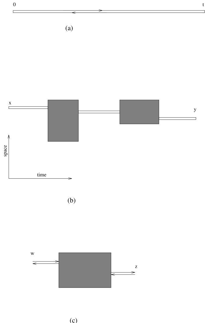
Figure 2: (a) A static unrenormalized meson propagator; (b) An excitation of the static unrenormalized meson propagator; (c) A close up of an intermediate excitation.

This tells us that the unrenormalized mass is $m_{0}=-log(4\tilde{k}_{f_{1}}\tilde{k}_{f_{2}})$. Let us now consider the effect on the mass produced by intermediate exited states. Fig. 2c shows an excitation, with the static propagator entering at the initial point $w$ and departing at the final point $z$. For fixed $w$ and $z$, we sum over all intermediate exited states to obtain the total weight for this event. We denote this weight by $D^{M}(w,z)$. The full propagator takes the form

$$\langle M(x)^{\dagger}M(y)\rangle = \sum_{n=0}^{\infty}\sum_{w_{i},z_{i}(i=1\dots n)}G_{0}^{{M}}(x,w_{1})D^{M}(w_{1},z_{1})G_{0}^{{M}}(z_{1},w_{2})D^{M}(w_{2},z_{2})\times$$ (17)

$$\times\dots\times D^{M}(w_{n},z_{n})G_{0}^{{M}}(z_{n},y)$$

where the points $w_{i}$ and $z_{i}$ are required to be time ordered and $n$ represents the number of excitations. This last equation is represented pictorially in Fig. 2b.

Following [15] one can factorize all static unrenormalized terms $G_{0}$ in eq (17) and compute the excitations $D(w_{i},z_{i})$ separately. We define

$$\tilde{D}^{M}(t)=(G_{0}^{M}(t))^{-1}\left.\sum_{x,y}D^{M}(x,y)\right|_{y_{0}-x_{0}=t}$$ (18)

where we normalize the excitation relative to the static unrenormalized propagator over the time interval $t$. From this definition and eq. (13) we obtain

$$G^{{M}}(t) = e^{-m_{0}t}\sum_{s_{i},t_{i}(i=1\dots n)}\tilde{D}^{M}(t_{1}-s_{1})\dots\tilde{D}^{M}(t_{n}-s_{n})=$$ (19)

$$\simeq e^{-m_{0}t}\,e^{p_{{M}}t}$$

where $t_{i}$ and $s_{i}$ are the corresponding time coordinates of $z_{i}$ and $w_{i}$. The exponential representation of (19) is up to an irrelevant boundary term exact and yields the renormalized mass $m_{{M}}$

$$m_{{M}}=m_{0}-p_{{M}}.$$ (20)

The mass correction $p_{M}$ can be written in the form

$$p_{{M}}=\sum_{z=(t^{\prime}\geq 0,\vec{z})}(G_{0}^{M}(t^{\prime}))^{-1}D^{M}(0,z)=\sum_{z=(t^{\prime}\geq 0,\vec{z})}(4k^{2})^{-t^{\prime}}D^{M}(0,z)\quad.$$ (21)

The last equation follows from (19) if we expand the exponential function containing $p_{M}$. The excitation term $D^{M}(w,z)$ is defined starting from eq. (13) in the following way:

$$D^{M}(w,z)=\frac{1}{A_{0}C_{M}}\sum_{\omega:w\mapsto z\mapsto w;\gamma\in S(\omega)}\,\,A(\omega,\gamma)\tilde{k}_{f_{1}}^{|\omega^{+}|}\tilde{k}_{f_{2}}^{|\omega^{-}|}\sum_{f_{sea}}\tilde{k}_{f_{sea}}^{|\gamma|}$$ (22)

where the sum is over all closed paths $\omega=\omega^{+}\cup\omega^{-}$ from $w$ to $z$ and $S(\omega)\subset\Lambda^{*}$ is the set of all loops $\gamma$ for with $\Omega(\omega,\gamma)\neq 0$. $A^{f_{1}f_{2}}(\omega,\gamma)$ denotes the amplitude of the intermediate excitations. $A_{0}=4$ is a constant which has to be explicitly evaluated from (13).

To evaluate the correction to the unrenormalized mass $m_{0}$ due to the excitations from eq. (21) we have to identify all closed paths $\omega$ from the point $0$ to the point $z=(t,\vec{z})$ and to sum over all points $\vec{z}$. At $\beta=0$ we do not have plaquettes in the expansion because the plaquette expectation value vanishes, therefore a diagram consists of a closed line $\omega=\omega^{+}\cup\omega^{-}$ composed by a set of connected bonds coming from the valence-quark contribution and a second path $\gamma$ coming from the sea-quark contribution. The group integral of a diagram is non-vanishing only if, for all $b\in\omega\cup\gamma$, there exists a second link $b^{\prime}\in\omega\cup\gamma$ such that $b=-b^{\prime}$ ($b$ is equal $b^{\prime}$ in opposite direction). A method to easily evaluate the group integral is discussed in [16].

4 Results and Conclusions

We now evaluate the mass of the pseudoscalar and the vector mesons with $f_{1}$ and $f_{2}$ quarks flavours up to order eight in the expansion, including valence and sea quarks. The sea quark contribution arises from quarks with the same flavour as the valence quarks, incorporated in the notation $k_{f_{1}},k_{f_{2}}$, as well as with flavours different from the valence quarks denoted by $k_{sea}$. All terms in the expression of the form $\left({{\it\tilde{k}_{f_{1}}}}^{n}+{{\it\tilde{k}_{f_{2}}}}^{n}+{{\it\tilde{k}_{sea}}}^{n}\right)$ with $n=4$ or $n=6$ correspond to sea quark contributions to the meson mass. Collecting all terms we obtain for the pseudoscalar meson mass

$$m_{PS}(\{\tilde{k}_{f_{1}}\tilde{k}_{f_{2}}\};\tilde{k}_{sea})=$$

$$-\ln(4\,{\it\tilde{k}_{f_{1}}}\,{\it\tilde{k}_{f_{2}}})-3\,{\it\tilde{k}_{f_{1}}}\,{\it\tilde{k}_{f_{2}}}-36\,{{\it\tilde{k}_{f_{1}}}}^{2}{{\it\tilde{k}_{f_{2}}}}^{2}-432\,{{\it\tilde{k}_{f_{1}}}}^{3}{{\it\tilde{k}_{f_{2}}}}^{3}$$

$$-3\,{{\it\tilde{k}_{f_{2}}}}^{2}\left({{\it\tilde{k}_{f_{1}}}}^{4}+{{\it\tilde{k}_{f_{2}}}}^{4}+{{\it\tilde{k}_{sea}}}^{4}\right)$$

$$-19\,{{\it\tilde{k}_{f_{1}}}}^{2}\left({{\it\tilde{k}_{f_{1}}}}^{4}+{{\it\tilde{k}_{f_{2}}}}^{4}+{{\it\tilde{k}_{sea}}}^{4}\right)-{\it\tilde{k}_{f_{1}}}\,{\it\tilde{k}_{f_{2}}}\,\left({{\it\tilde{k}_{f_{1}}}}^{4}+{{\it\tilde{k}_{f_{2}}}}^{4}+{{\it\tilde{k}_{sea}}}^{4}\right)$$

$$-5328\,{{\it\tilde{k}_{f_{1}}}}^{4}{{\it\tilde{k}_{f_{2}}}}^{4}-8\,{{\it\tilde{k}_{f_{1}}}}^{2}\left({{\it\tilde{k}_{f_{1}}}}^{6}+{{\it\tilde{k}_{f_{2}}}}^{6}+{{\it\tilde{k}_{sea}}}^{6}\right)-8\,{{\it\tilde{k}_{f_{2}}}}^{2}\left({{\it\tilde{k}_{f_{1}}}}^{6}+{{\it\tilde{k}_{f_{2}}}}^{6}+{{\it\tilde{k}_{sea}}}^{6}\right)$$

$$-16\,{\it\tilde{k}_{f_{1}}}\,{\it\tilde{k}_{f_{2}}}\,\left({{\it\tilde{k}_{f_{1}}}}^{6}+{{\it\tilde{k}_{f_{2}}}}^{6}+{{\it\tilde{k}_{sea}}}^{6}\right)-32\,{\it\tilde{k}_{f_{1}}}\,{{\it\tilde{k}_{f_{2}}}}^{3}\left({{\it\tilde{k}_{f_{1}}}}^{4}+{{\it\tilde{k}_{f_{2}}}}^{4}+{{\it\tilde{k}_{sea}}}^{4}\right)$$

$$-32\,{{\it\tilde{k}_{f_{1}}}}^{3}{\it\tilde{k}_{f_{2}}}\,\left({{\it\tilde{k}_{f_{1}}}}^{4}+{{\it\tilde{k}_{f_{2}}}}^{4}+{{\it\tilde{k}_{sea}}}^{4}\right)-48\,{{\it\tilde{k}_{f_{1}}}}^{2}{{\it\tilde{k}_{f_{2}}}}^{2}\left({{\it\tilde{k}_{f_{1}}}}^{4}+{{\it\tilde{k}_{f_{2}}}}^{4}+{{\it\tilde{k}_{sea}}}^{4}\right)$$

$$+8\,{{\it\tilde{k}_{f_{2}}}}^{4}\left({{\it\tilde{k}_{f_{1}}}}^{4}+{{\it\tilde{k}_{f_{2}}}}^{4}+{{\it\tilde{k}_{sea}}}^{4}\right)+8\,{{\it\tilde{k}_{f_{1}}}}^{4}\left({{\it\tilde{k}_{f_{1}}}}^{4}+{{\it\tilde{k}_{f_{2}}}}^{4}+{{\it\tilde{k}_{sea}}}^{4}\right)$$

and for the vector meson mass

$$m_{VK}(\{\tilde{k}_{f_{1}}\tilde{k}_{f_{2}}\};\tilde{k}_{sea})=$$

$$-\ln(4\,{\it\tilde{k}_{f_{1}}}\,{\it\tilde{k}_{f_{2}}})-2\,{\it\tilde{k}_{f_{1}}}\,{\it\tilde{k}_{f_{2}}}-16\,{{\it\tilde{k}_{f_{1}}}}^{2}{{\it\tilde{k}_{f_{2}}}}^{2}-128\,{{\it\tilde{k}_{f_{1}}}}^{3}{{\it\tilde{k}_{f_{2}}}}^{3}$$

$$-3\,{{\it\tilde{k}_{f_{2}}}}^{2}\left({{\it\tilde{k}_{f_{1}}}}^{4}+{{\it\tilde{k}_{f_{2}}}}^{4}+{{\it\tilde{k}_{sea}}}^{4}\right)$$

$$-19\,{{\it\tilde{k}_{f_{1}}}}^{2}\left({{\it\tilde{k}_{f_{1}}}}^{4}+{{\it\tilde{k}_{f_{2}}}}^{4}+{{\it\tilde{k}_{sea}}}^{4}\right)-{\it\tilde{k}_{f_{1}}}\,{\it\tilde{k}_{f_{2}}}\,\left({{\it\tilde{k}_{f_{1}}}}^{4}+{{\it\tilde{k}_{f_{2}}}}^{4}+{{\it\tilde{k}_{sea}}}^{4}\right)$$

$$-1088\,{{\it\tilde{k}_{f_{1}}}}^{4}{{\it\tilde{k}_{f_{2}}}}^{4}-8\,{{\it\tilde{k}_{f_{1}}}}^{2}\left({{\it\tilde{k}_{f_{1}}}}^{6}+{{\it\tilde{k}_{f_{2}}}}^{6}+{{\it\tilde{k}_{sea}}}^{6}\right)-8\,{{\it\tilde{k}_{f_{2}}}}^{2}\left({{\it\tilde{k}_{f_{1}}}}^{6}+{{\it\tilde{k}_{f_{2}}}}^{6}+{{\it\tilde{k}_{sea}}}^{6}\right)$$

$$-16\,{\it\tilde{k}_{f_{1}}}\,{\it\tilde{k}_{f_{2}}}\,\left({{\it\tilde{k}_{f_{1}}}}^{6}+{{\it\tilde{k}_{f_{2}}}}^{6}+{{\it\tilde{k}_{sea}}}^{6}\right)-24\,{\it\tilde{k}_{f_{1}}}\,{{\it\tilde{k}_{f_{2}}}}^{3}\left({{\it\tilde{k}_{f_{1}}}}^{4}+{{\it\tilde{k}_{f_{2}}}}^{4}+{{\it\tilde{k}_{sea}}}^{4}\right)$$

$$-24\,{{\it\tilde{k}_{f_{1}}}}^{3}{\it\tilde{k}_{f_{2}}}\,\left({{\it\tilde{k}_{f_{1}}}}^{4}+{{\it\tilde{k}_{f_{2}}}}^{4}+{{\it\tilde{k}_{sea}}}^{4}\right)-32\,{{\it\tilde{k}_{f_{1}}}}^{2}{{\it\tilde{k}_{f_{2}}}}^{2}\left({{\it\tilde{k}_{f_{1}}}}^{4}+{{\it\tilde{k}_{f_{2}}}}^{4}+{{\it\tilde{k}_{sea}}}^{4}\right)$$

$$+8\,{{\it\tilde{k}_{f_{2}}}}^{4}\left({{\it\tilde{k}_{f_{1}}}}^{4}+{{\it\tilde{k}_{f_{2}}}}^{4}+{{\it\tilde{k}_{sea}}}^{4}\right)+8\,{{\it\tilde{k}_{f_{1}}}}^{4}\left({{\it\tilde{k}_{f_{1}}}}^{4}+{{\it\tilde{k}_{f_{2}}}}^{4}+{{\it\tilde{k}_{sea}}}^{4}\right)$$

To fix the quark masses we use the experimental values of meson masses expressed in units of the $\rho$ mass. For the u- , d- and s- quark masses we use the experimental pion and kaon masses (we consider the u- and the d- quarks to have the same mass). For this evaluation we neglect all sea quarks of flavour different from u, d and s. We thus obtain two equations

$$\frac{m_{PS}(\{k_{u}=k_{d}\};k_{sea}=k_{s})}{m_{VK}(\{k_{u}=k_{d}\};k_{sea}=k_{s})}=\frac{m_{\pi}}{m_{\rho}}\simeq 0.18$$ (25)

$$\frac{m_{PS}(\{k_{u},k_{s}\};k_{sea}=0)}{m_{VK}(\{k_{u}=k_{d}\};k_{sea}=k_{s})}=\frac{m_{K}}{m_{\rho}}\simeq 0.64$$ (26)

from which we can extract the values of $k_{u}$ and $k_{s}$ . The resulting values are $k_{u}=k_{d}=0.28(3)$ and $k_{s}=0.25(2)$. The error given here is an estimate of the systematic error from the truncation of the expansion. It was obtained by comparing the truncated results to the known bounds in the meson masses [12]

$$m_{PS}\leq-\log(4k^{2})-\frac{3k^{2}}{1-12k^{2}}\hskip 28.45274ptm_{VK}\leq-\log(4k^{2})-\frac{2k^{2}}{1-8k^{2}}\hskip 28.45274pt$$ (27)

where $k={\rm max}(k_{f_{1}},k_{f_{2}},k_{sea})$.

Using these parameters one can check the expansion by predicting the $K^{*}$ mass obtained from the vector meson mass formula

$$\frac{m_{VK}(\{k_{u}=0.28,k_{s}=0.25\};k_{sea}=0)}{m_{VK}(\{k_{u}=k_{d}=0.28\};k_{sea}=k_{s})}=1.25(12)$$ (28)

which compares favourably with the experimental value of $m_{K^{*}}/m_{\rho}\simeq 1.16$. Knowing the u- and s- quark masses one can estimate the ratio of the $\bar{s}s$ to $\bar{u}u$ condensates in the vaccum. To order eight it is easy to compute and we find $<\bar{s}s>/<\bar{u}u>=\left(k_{s}/k_{u}\right)^{8}$. Because this depends on the eighth power of the $k-$ values it is very sensitive on the errors of $k_{u}$ and $k_{s}$.

In an analogous way one fixes the c-quark mass using the experimental value of the $D$- meson mass. The accuracy of the expansion can then be checked by comparing the predicted mass of the $D^{*}$ with the experimental value. In this case we find $k_{c}=0.14(1)$ leading to a $D^{*}$ meson mass ratio $m_{D^{*}}/m_{\rho}$ of 2.5(1) to be compared with the experimental value of 2.62.

Having fixed the quark masses we obtain for the ratio

$$\left.\frac{\langle D|\bar{u}u|D\rangle}{\langle D|\bar{s}s|D\rangle}=\frac{\partial m_{PS}(\tilde{k}_{u};k_{c}=0.14;k_{sea}=k_{s})/\partial\lambda_{u}}{\partial m_{PS}(k_{u}=0.28;k_{c}=0.14;\tilde{k}_{s})/\partial\lambda_{s}}\right|_{\tilde{k}_{u}=0.28;\tilde{k}_{s}=0.25}\simeq 50(10)$$ (29)

The error given for the ratio is estimated by taking into account only the errors in the values of the $k$’s which include part of the systematic error due to the truncation. The latter can not be estimated in the same way as the error in the $k$’s because no upper bounds exist for the derivative of the meson mass.

The same analysis can also be done in the case of the B- meson where one uses the experimental value of the $B$- meson mass to fix $k_{b}$. We find $k_{b}=0.011(2)$ leading to a $B^{*}$ meson mass ratio $m_{B^{*}}/m_{\rho}$ of 6.8(4) within the experimental value of 7.06 and for the ratio

$$\frac{\langle B|\bar{u}u|B\rangle}{\langle B|\bar{s}s|B\rangle}\simeq 45(5)\quad.$$ (30)

We note that, for the allowed parameter range $(k_{u},k_{f},k_{s})\in[0,0.28]^{3}$ where $k_{f}$ is the hopping parameter corresponding to the c- or the b- quark the ratios (29,30) remain bounded from below by

$$\frac{\langle M|\bar{u}u|M\rangle}{\langle M|\bar{s}s|M\rangle}>40~{}~{}~{}~{}\forall(k_{u},k_{f},k_{s})\in[0,0.28]^{3}\quad.$$ (31)

From the above values of the ratios we conclude that the non-valence contribution in the D- and B- mesons is suppressed compared to the valence contribution by at least an order of magnitude. This would comply with the OZI rule meaning that the OZI rule can not be evaded in the limit of infinite coupling. Therefore the enhancement observed in D- meson decays to strange final states seems not to be explained by a rich $\bar{s}s$ content in the D-meson. Whether finite $\beta$ effects can change the above ratio by an order of magnitude can only be checked by doing a finite $\beta$ lattice simulation.

Acknowledgements: We thank M. Karliner for the initial motivation for this work and interesting comments as well as F. Jegerlehner for a careful reading of the manuscript.

References

[1] European Muon Collaboration, J. Ashman et al, Phys. Lett
B 206 (1988) 364; Nucl. Phys. B 328 (1990) 1
[2] New Muon Collaboration, P. Amaudruz al, Phys. Rev. Lett
66 (1991) 2712; M. Arneodo et al, Phys. Rev D 50 (1994) R1
[3] NA51 Collaboration, A. Baldit et al, Phys. Lett B 332 (1994) 244
[4] J. Ellis, M. Karliner, D. E. Kharzeev and M. G. Sapozhnikov,
CERN preprint CERN-TH.7326/94 hep-ph/9412334
[5] M. Fukugita, Y. Kuramashi, M. Okawa and A. Ukawa, Phys. Rev.
D 51 (1995) 5319
[6] S. Dong and H. Liu, Nucl. Phys B (Proc. Supl.) 42 (1995)
322
[7] J. Gasser, H. Leutwyler and M. E. Sainio, Phys Lett. B 253
(1991) 252
[8] J. Ellis, Y. Frishman, A. Hanny and M. Karliner, Nucl. Phys. B
382 (1992) 189
[9] E769 Collaboration, G. A. Alves et al, Phys. Rev.
Lett. 72 (1994) 812, Erratum-ibid. 72 (1994) 1946;
WA82 Collaboration, M.
Adamovich et al, Phys. Lett. B 305 (1993) 402;
Tagged Photon Spectrometer Collaboration, J. C. Anjos
et al Phys. Rev. Lett. 69 (1992) 2892;
M. Bauer, B. Stech and M. Wirbel, Z. Phys. C33 (1987) 561
[10] N.Kawamoto, Nucl. Phys. B190 (1981) 617
[11]N.Kawamoto and K.Shigemoto, Nucl. Phys. B237 (1984) 128
[12] A.Galli, PSI-PR-94-33
[13] J.Hoek and J.Smit, Nucl. Phys. B263 (1986) 129
[14] K.Wilson, Phys. Rev. D10 (1974) 2445
[15] J. Fröhlich and C. King, Nucl. Phys. B 290 (1980) 504