SWAT/75

A Cluster Algorithm for the $Z_{2}$ Kalb-Ramond Model.

P. K. Coyle and I. G. Halliday

Department of Physics

University of Wales, Swansea

Singleton Park

Swansea, SA2 8PP, U.K.

1 Introduction

The standard local algorithms [1] for updating monte-carlo simulations become very inefficient when applied to systems near a phase transition. As the critical point is approached correlation lengths diverge signifying large scale structures on the lattice. These structures make simulations much more difficult. In order to significantly change the relevant objects, lattice variables with large separations have to be changed coherently.

As the linear size (and therefore correlation lengths at criticality) is increased the algorithm has to be applied more times to achieve a statistically independent configuration. Thus as the lattice size is increased not only will each update take longer but many more updates will be needed.

Cluster algorithms try to address this problem by identifying the structures relevant to the dynamics of the phase transition and using them as the dynamical variables. In this way it is possible to construct an algorithm which acts directly on the relevant objects while still producing configurations with the correct statistical weight.

Cluster methods were first introduced for the Ising model [2, 3] and have since been extended to other spin models, in some cases reducing the critical exponent to near zero. Attempts to apply the same principles to gauge theories have been successful for some models such as the $Z_{2}$ gauge theory in three dimensions [4] and some vertex models [5]. However simulations of other gauge groups, like SU(3), near criticality remain plagued by Critical slowing down.

The $Z_{2}$ plaquette theory [6, 7], being the centre of SU(2) is thought to be responsible for the phase transition seen in its adjoint representation, and therefore closely related to the second order point in the fundamental-adjoint phase diagram [8, 9].

In [4] Ben-Av et.al. showed that the dynamics governing the phase transition in a three dimensional $Z_{2}$ gauge theory is governed by gauge independent vortex loops and developed an algorithm to stochastically update these loops and thus dramatically reduce critical slowing down. Here we will show that these techniques can be extended to the 4 dimensional $Z_{2}$ plaquette theory where the dynamics are very similar.

2 The Model

The dynamical variables $P_{x,\mu\nu}$ are defined on the plaquettes of a 4 dimensional hyper-cubic lattice and can take on values $\pm 1$. The action is defined on 3 dimensional hypercubes $C$ and is given by:

$${\rm S}={\sum_{C}{\rm S_{c}(\delta C)}}$$ (1)

where

$${\rm S_{c}(\delta C)}={-\prod_{\delta C}P_{x,\mu\nu}}$$ (2)

and $\delta C$ are the plaquettes on the surface of the cube $C$.

Each 3-cube has a value of $\pm 1$ and corresponds to a link on the dual lattice. Configurations can be uniquely defined, up to a gauge transformation by the links on the dual lattice. The bianchi identity for this model constrains the dual lattice configuration to be a system of frustrated (-1) dual link loops embedded in a sea of satisfied (+1) dual links. These dual loops are the world lines of monopoles [6].

This conserved monopole current $M_{z}^{\sigma}$ is given by

$$M_{z}^{\sigma}=\epsilon^{\sigma\rho\mu\nu}\Delta_{\rho}P_{x,\mu\nu}$$ (3)

with

$$\Delta_{\sigma}M_{z}^{\sigma}=0$$ (4)

Here $M_{z}^{\sigma}$ lies on links of the dual lattice and z labels the dual site corresponding to the hypercube at x. Integrating $P_{x,\mu\nu}$ around a 3-cube gives

$$M_{z}^{\sigma}=\oint P_{x,\mu\nu}\partial C$$ (5)

Summing this over all 3-cubes (or dual links) gives the monopole world line density which is equivalent to the Gibbs free energy.

This model is dual to the 4 dimensional Ising model which has been extensively studied [10] and gives the most accurate value for the $Z_{2}$ phase transition at $\beta=0.953$.

3 The Algorithm

The algorithm used is a single cluster [3] update performed on the dual lattice (ie on the 3-cubes) and is therefore gauge invariant. It follows the same structure as the 3 dimensional case [4].

The algorithm works by modifying the path taken by the monopole world lines using the Boltzmann factor to weight any changes to the configuration. A random starting point is chosen to build a tree of possible paths. This tree is called the graph of deletions. Fig.1 gives an example of how such a tree would be constructed (the example has been restricted to 2 dimensions for clarity).

         

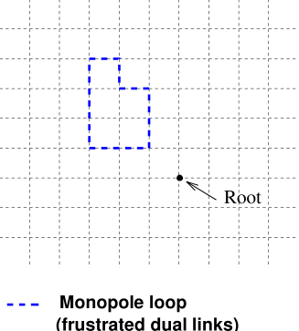
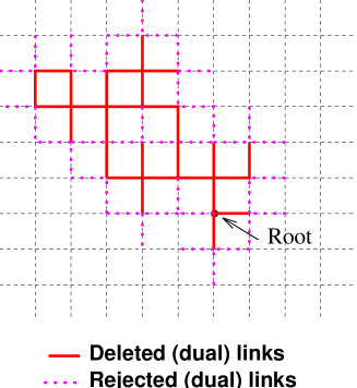
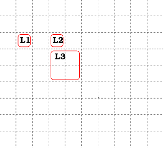
Figure 1: a) The initial monopole configuration and a randomly picked root. b) A graph of deletions built from the root. c) The three loops which can be updated independently.

Starting with the previous configuration pick a random point to be the root (Fig.1a). Visit each direction and add the neighbouring node with probability

$$P_{d}=e^{\beta(S_{c}-1)}$$ (6)

Thus if an existing loop is encountered it is automatically added to the graph of deletions. Non-frustrated dual links are added with a probability dependent on the coupling $\beta$. (Fig.1b) shows a possible graph of deletions. All dual links not in the graph of deletions are frozen.

The bianchi identity can be used to uniquely update the external legs of the tree as valid configurations can only contain closed loops (Fig.1c). The only degrees of freedom left for changing the deleted links is a random choice of turning each loop on or off. That is choosing the links in each loop to be frustrated (on) or satisfied (off). Fig.2 shows 4 of the new configurations which are possible by updating the graph of deletions. The remaining 4 possibilities have L1 turned off. Each outcome is weighted equally.

Figure 2: 4 of the 8 configurations possible from this graph of deletions. The other 4 have L1 turned off.

Using the language of Kandel and Domany [11] the dual links forming the cluster are said to be deleted and form a graph of deletions. All other dual links are frozen. In this language the graph of deletions is updated by randomly choosing a new monopole configuration which does not change any of the frozen dual links.

It is easy to see how the algorithm can modify or even destroy an existing monopole loop while also being able to create new loops of arbitrary size.

The algorithm can easily be implemented on a computer as follows.

1. Pick a random dual site (Hypercube) to be the root of the graph of deletions.

2. Visit each dual link (3-cube) connected to this site and add it to the graph of deletions with probability $P_{d}=e^{\beta(S_{c}-1)}$. These links are said to be deleted.

3. Keep repeating the above step for each of the newly added dual sites until all of the dual links connected to the graph of deletions have been visited making sure that each dual link is only ever visited once.

4. Identify all the loops within the graph of deletions and choose one dual link for each loop to be a free link. This leaves a spanning tree.

5. Randomly assign a value to each of the free links.

6. All remaining links in the spanning tree are constrained so the bianchi identity can be used to update each link in the tree and create a valid configuration.

The algorithm is obviously ergodic as there is a finite probability of deleting all of the dual links and choosing a completely random configuration from the set of all valid configurations. Detailed balance also follows along the usual lines.

4 Measurements and error analysis

To measure how effective the algorithm is at producing independent configurations we calculated the normalised autocorrelation function (7) for the Monopole density $M$.

$$A_{M}(t)={{<M_{s}M_{s+t}>-<M>^{2}}\over{<M_{s}^{2}>-<M>^{2}}}$$ (7)

Integrating (7) gives the integrated autocorrelation time $\tau_{int}$ (8) .

$$\tau_{int,M}={1\over 2}\sum_{t=-\infty}^{+\infty}A_{M}(t)$$ (8)

$\tau_{int}$ measures how many more updates are needed due to the configurations not being independent. For a sample mean:

$$\bar{M}={1\over n}\sum_{t=1}^{n}M_{t}$$ (9)

the variance in $\bar{M}$ is

$$Var(\bar{M})={1\over n}2\tau_{int}{(<M_{s}^{2}>-<M>^{2})}$$ (10)

for $n>>\tau$. This is $2\tau_{int}$ times larger than expected for independent configurations.

The Autocorrelation function decays exponentially at least for large $s$. Fitting the tail of (7) to an exponential gives $\tau_{exp}$ the exponential autocorrelation time. $\tau_{int}$ is defined so as to make $\tau_{int}\approx\tau_{exp}$ for large $\tau$. The autocorrelation time diverges as a power of the correlation length so at the critical point $\tau$ varies with the lattice size L as:

$$\tau\approx L^{z}$$ (11)

The critical exponent $z$ quantifies the extent to which critical slowing down is affecting the simulation. Local algorithms tend to have $z\approx 2$ for models with a phase transition.

5 Results

Simulations were performed on Dec 3400AXP Workstations. For comparison a standard Metropolis algorithm was also studied. The monopole density (3) was calculated after each update. A number of simulations were performed for $\beta$ values around the critical point in order to find the largest autocorrelation time for the lattice size. Both exponential ($\tau_{exp}$) and integrated ($\tau_{int}$) autocorrelation time were measured for the Monopole density. Both were found to be in agreement although for the cluster algorithm $\tau_{exp}$ proved easier to calculate as the autocorrelation functions fitted a exponential very closely before the tail became too noisy. Errors in the autocorrelation function were calculated using blocking. We noticed auto-correlation functions for metropolis were not pure exponentials. To fit this to an exponential decay it was necessary to find a window in the autocorrelation function after an initial power law dependence but before noise takes over. Metropolis gave a critical exponent of $z_{c}>2$ as expected for a local algorithm.

As our algorithm only updates one cluster at a time the effect of each application can vary from updating no links to updating the entire lattice. In order to make a useful comparison of the CPU requirements for each algorithm the sweeps of the cluster algorithm were scaled by a factor $C$ representing the average cluster size. This factor was calculated as follows. Each application of the algorithm is said to be one hit. This hit touches $C$ dual links of the lattice. $S$ of these links form the spanning tree. $F$ are free links. $R$ links are looked at but rejected. The graph of deletions therefore contains $S+F$ links. Fig.1 shows the CPU load is roughly proportional to the cluster size $C$ which we have defined as $C=S+F+R$.

Figure 3: A comparison of Cluster sizes and CPU requirements for a $5^{4}$ lattice

One sweep of the lattice is defined as $N/C$ hits where $N$ is the total number of links on the lattice. Thus a sweep takes approximately the same time for all $\beta$ and each dual link is touched on average once per sweep. Each Cluster sweep took approximately the same time as a metropolis sweep. The extra complexity is compensated for by working on the smaller dual lattice where it is easier to calculate the action. Our code for metropolis updated approximately $0.42\times 10^{6}$ plaquettes/s a second while the cluster algorithm updates approximately $0.3\times 10^{6}$ dual links/s.

Runs consisted of $1\times 10^{6}$ — $2\times 10^{6}$ clusters which gives approximately $6\times 10^{4}$ — $6\times 10^{5}$ sweeps. Fig 5 shows the results for the autocorrelation time $\tau_{int}$ against lattice size. The solid lines are our best fits of $z_{c}=0.32\pm 0.06$ for the cluster algorithm and $z_{c}=2.58\pm 0.1$ for metropolis.

Figure 4: Monte-carlo simulations of $Z_{2}$ Kalb-Ramond model in 4D using Metropolis and Cluster algorithms. Autocorrelation time vs Lattice size.

6 Conclusions

The Cluster algorithm presented above becomes more efficient than Metropolis for lattice sizes as small as $4^{4}$ and is approximately 1000 times more efficient for a $15^{4}$ lattice. Comparing our algorithm to Wolff’s for the 4D Ising model gives further support to the idea of universality classes. You can see from Table 1 that dynamical critical exponents for the $Z_{2}$ models and their corresponding dual Ising models are the same within errorbars.

The embedding of Ising spins has been used successfully to extended the realm of cluster algorithms to other spin systems although not all embeddings work [12]. It is hoped that embedding this $Z_{2}$ algorithm in a full $SU(2)$ theory will give some insight into the structure of the $SU(2)$ fundamental-adjoint phase diagram [8, 9, 13, 14, 15] and the bulk transition of pure SU(2).

Model	Swendsen–Wang	Single Cluster
$Z_{2}$ 4D	—	$0.32\pm 0.06$
Ising 4D	$0.83\pm 0.01$	$0.29\pm 0.07$
$Z_{2}$ 3D	$0.73\pm 0.06$	—
Ising 3D	$0.75\pm 0.01$	$0.39\pm 0.01$

Table 1: Dynamical Critical Exponents for $Z_{2}$ models and the Ising models to which they are dual.

References

- [1] N.Metropolis A.W.Rosenbluth M.N.Rosenbluth A.H.Teller and E.Teller. J.Chem.Phys., 21:1087, 1953.
- [2] R.H.Swendsen and J.S.Wang. Phys.Rev.Lett., 58:89, 1987.
- [3] U.Wolff. Phys.Rev.Lett., 62:361, 1981.
- [4] R.Ben-Av D.Kandel E.Katznelson P.G.Lawers and S.Solomon. J.Stat.Phys., 58:125, 1990.
- [5] H.G.Evertz and M.Marcu. Lattice’92, page 277, 1992.
- [6] M.Kalb and P.Ramond. Phys.Rev., D9:2273, 1974.
- [7] F.J.Wegner. ,J.Math.Phys., 12:2259, 1971.
- [8] I.G.Halliday and A.Schwimmer. Phys.Lett., 101B:327, 1981.
- [9] I.G.Halliday and A.Schwimmer. Phys.Lett., 102B:337, 1981.
- [10] I.Montvay and P.Weisz. Nucl.Phys., B290:327, 1987.
- [11] D.Kandel and E.Domany. Phys.Rev., B43:8539, 1991.
- [12] S.Caracciolo R.G.Edwards A.Pelissetto A.D.Socal. Nucl.Phys., B403:475, 1993.
- [13] I.G.Halliday L.Caneschi and A.Schwimmer. Phys.Lett., 117B:427, 1982.
- [14] M.Mathur R.Gavai and M.Grady 1994. hep-lat/9410004, 1994.
- [15] M.Mathur and R.Gavai. Nucl.Phys., B423:123, 1994.