UTHEP-304

UTCCP-P-1

May 1995

QCD Phase Transition with Strange Quark
in Wilson Formalism for Fermions

Y. Iwasaki,^a,b K. Kanaya,^a,b S. Kaya,^a S. Sakai,^c and T. Yoshié^a,b

^a Institute of Physics, University of Tsukuba, Ibaraki 305, Japan
^b Center for Computational Physics, University of Tsukuba,
Ibaraki 305, Japan
^c Faculty of Education, Yamagata University, Yamagata 990, Japan

The nature of QCD phase transition is studied with massless up and down quarks and a light strange quark, using the Wilson formalism for quarks on a lattice with the temporal direction extension $N_{t}=4$. We find that the phase transition is first order in the cases of both about 150 MeV and 400 MeV for the strange quark mass. These results together with those for three degenerate quarks suggest that QCD phase transition in nature is first order.

One of major goals of numerical studies of lattice QCD is to determine the nature of the phase transition from the high temperature quark-gluon-plasma phase to the low temperature hadron phase, which is supposed to occur at the early stage of the Universe and possibly at heavy ion collisions. It is, in particular, crucial to know the order of the transition to understand the evolution of the Universe. Because the critical temperature is of the same order of magnitude as the strange quark mass, we have to take into account the effect of the strange quark as well as those of almost massless up and down quarks. In this article we study the nature of QCD phase transition with these three quarks in the Wilson formalism of fermions on the lattice. The investigation using Wilson quarks is highly important, because the Wilson formalism of fermions on the lattice is the only known formalism which possesses a local action for any number of flavors with arbitrary quark masses. Preliminary reports are given in [1].

The results of numerical simulations with Wilson quarks [2] as well as with staggered quarks [3] imply that the chiral phase transition is second order for two massless quarks, while it is first order for three. This is also consistent with theoretical predictions based on universality [4]. In a numerical study we are able to vary the mass of the strange quark. When the mass of the strange quark is reduced from infinity to zero, the phase transition must change from second order to first order at some quark mass $m_{s}^{*}$. This is a tricritical point. The crucial point is whether the physical strange quark mass is larger or smaller than $m_{s}^{*}$.

The action we use in this article is composed of the standard one-plaquette gauge action with the gauge coupling constant $g$ ($\beta=6/g^{2}$) and the Wilson quark actions for u, d and s quarks with the hopping parameters $K_{u}$, $K_{d}$ and $K_{s}$, respectively. We set $K_{u}=K_{d}$.

We perform simulations on lattices of the temporal extension $N_{t}=4$ with the spatial sizes $8^{2}\times 10$ and $12^{3}$. Although $N_{t}=4$ is not large enough to obtain the result for the continuum limit, this work is a first step toward the understanding of the nature of the QCD phase transition with Wilson quarks. We generate gauge configurations by the hybrid R algorithm with a molecular dynamics step $\Delta\tau=0.01$ and a trajectory of unit time. The inversion of the quark matrix is made by a minimal residual method or a conjugate gradient method. When the hadron spectrum is calculated, the lattice is duplicated in the direction of lattice size 10 or 12. We use an anti-periodic boundary condition for quarks in the $t$ direction and periodic boundary conditions otherwise. The statistics is in general total $\tau=$ several hundreds, and the plaquette and the Polyakov loop are measured every simulation time unit and hadron spectrum is calculated every $\delta\tau=5$ (or 10 sometimes). When the value of $\beta$ is small, the fluctuation of physical quantities are small and therefore we think the statistics is sufficient for the purpose of this article.

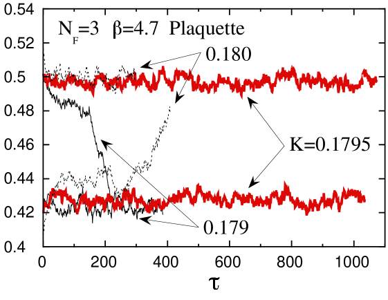
Figure 1: Time history of the plaquette for $N_{F}=3$ at (a) $\beta=4.7$ and (b) 5.0 on a $12^{3}\times 4$ lattice.

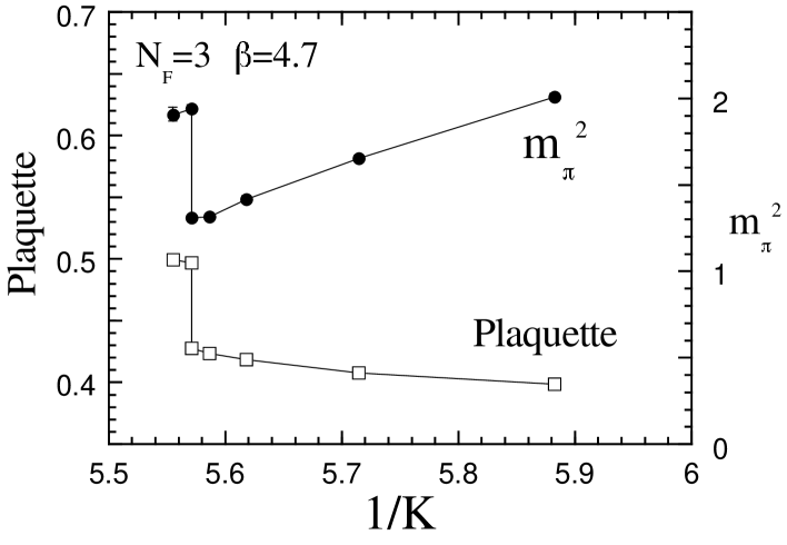
Figure 2: $(m_{\pi}a)^{2}$ and the plaquette for $N_{F}=3$ at $\beta=4.7$.

Let us first discuss the results for the degenerate $N_{F}=3$ case: $K_{u}=K_{d}=K_{s}\equiv K$. In order to find the transition/crossover points we perform simulations at $\beta$=4.0, 4.5, 4.7, 5.0 and 5.5. The simulation time history of the plaquette at $\beta=4.7$ on a $4\times 12^{3}$ lattice is plotted in Fig. 1(a). The low and high temperature phases coexist over 1,000 trajectories at $K=0.1795$ and in accord with this we find two-state signals also in other observables such as the plaquette and $m_{\pi}^{2}$ (Fig. 2). From them we conclude that the transition at $K=0.1795(5)$ and $\beta=4.7$ is first order. The transition/crossover points thus identified are summarized in Table 1.

In a previous paper [2] we reported a clear two-state signal in the chiral limit $K_{c}=0.235$ at $\beta=3.0$ for $N_{F}=3$. An interesting question is to determine the critical value of the quark mass $m_{q}^{crit}$ up to which the first order phase transition persists. We observed clear two state signals at $\beta$ = 4.0, 4.5 and 4.7, while for $\beta=5.0$ and $5.5$ no such signals have been seen (see Fig. 1(b) for the time history of the plaquette at $\beta=5.0$). At the transition point (in the confining phase) of $\beta=4.7$ the value of $m_{q}a$ is 0.175(2) and $(m_{\pi}/m_{\rho})=0.873(6)$. The quark mass is defined through the axial Ward identity [5] for Wilson quarks. The results of the hadron spectrum in the range of $\beta=3.0$ – 4.7 for $N_{F}=2$ and 3 (Fig. 3) indicate that the inverse lattice spacing $a^{-1}$ estimated from the $\rho$ meson mass is almost independent on $\beta$ in this range and $a^{-1}\sim 0.8$ GeV. Therefore we obtain a bound on the critical quark mass $m_{q}^{crit}\mathop{\vtop{\halign{#\cr$\hfil\displaystyle{>}\hfil$\crcr\kern 0.5pt\nointerlineskip\cr$\sim$\crcr\kern 0.5pt\cr}}}\limits 140$ MeV, or equivalently $(m_{\pi}/m_{\rho})^{crit}\geq 0.873(6)$.

We note that these values are much larger than those for the staggered fermion case for which $m_{q}^{crit}\sim 10$ – 40 MeV ($m_{q}^{crit}a=0.025$ – 0.075 [6, 7]. We have used $a^{-1}\sim 0.5$ GeV at $\beta=5.2$ for $N_{F}$=2[8]) and $(m_{\pi}/m_{\rho})^{crit}\simeq 0.42$ – 0.58 (the result for $N_{F}=4$ at $\beta=5.2$[9], because the data for $N_{F}=3$ are not available.)

Now let us discuss a more realistic case of massless u and d quarks and a light s quark ($N_{F}=2+1$). Our strategy to investigate this problem is similar to that we utilized in our previous work [2] for the investigation of the chiral transition in the degenerate quark mass cases, which we call “on-$K_{c}$” simulation method. We set the value of the masses of u and d quarks $m_{ud}$ to zero ($K_{u}=K_{d}=K_{c}$) and fix the s quark mass $m_{s}$ to some value, and make simulations reducing the value of $\beta$ starting from a deconfining phase. When u and d quarks are massless, the number of iteration $N_{\rm inv}$ needed for the quark matrix inversion (for u and d quarks) is enormously large in the confining phase, while it is of order of several hundreds in the deconfining phase. This is due to the fact that there are zero modes around $K_{c}$ in the low temperature phase, while none exists in the high temperature phase [10]. Therefore the $N_{\rm inv}$ provides an extremely good indicator to discriminate the two phase when u and d quarks are on the $K_{c}$ line. Combining this with measurements of physical observables, we identify the transition point and determine the order of the transition.

The values which we take for $K_{c}$ are given in Table 2. They are the vanishing point of extrapolated $m_{\pi}^{2}$ for $N_{F}=2$ and interpolated ones. We have used those for $N_{F}=2$, because we have the data most in this case, and the difference between that for $N_{F}=3$ and for $N_{F}=2$ is of the same order of magnitude as the difference due to the definition of $K_{c}$, either the vanishing point of $m_{q}$ or $m_{\pi}^{2}$ [2].

We study two cases of $m_{s}\sim 150$ MeV and 400 MeV. From the value of $a^{-1}\sim 0.8$ GeV and an empirical rule $m_{q}a\simeq(2/3)(1/K-1/K_{c})$ satisfied in the $\beta$ region we have studied (Fig. 3), we get the values for $K_{s}$ shown in Table 2. It should be noted that the physical s quark mass determined from $m_{\phi}=1020$ MeV turns out to be $m_{s}\sim 150$ MeV in this $\beta$ range for our definition of the quark mass.

The simulation time history of $N_{\rm inv}$ on the $8^{2}\times 10$ spatial lattice is plotted in Fig. 4(a) for the case of 150 MeV. When $\beta\geq 3.6$, $N_{\rm inv}$ is of order of several hundreds, while when $\beta\leq 3.4$, $N_{\rm inv}$ shows a rapid increase with $\tau$. At $\beta=3.5$ we see a clear two-state signal depending on the initial condition: For a hot start, $N_{\rm inv}$ is quite stable around $\sim 900$ and $m_{\pi}^{2}$ is large ($\sim 1.0$ in lattice units). On the other hand, for a mix start, $N_{\rm inv}$ shows a rapid increase with $\tau$ and exceeds 2,500 in $\tau\sim 10$, and in accord with this, the plaquette and $m_{\pi}^{2}$ decreases with $\tau$ as shown in Fig. 4(b) for the plaquette. For the case of 400 MeV a similar clear two-state signal is observed at $\beta=3.9$ both on the $8^{2}\times 10$ and $12^{3}$ spatial lattices (Fig. 5). Thus the method of “on-$K_{c}$” simulation is very powerful to identify the point of the transition, although in the low temperature phase we are only able to obtain upper (or lower) bounds of physical observables. The values of $m_{\pi}^{2}$ versus $\beta$ are plotted in Fig. 6 together with those in the case of degenerate $N_{F}=3$ on the $K_{c}$ line [2]. At $\beta=3.5$ for the case of 150 MeV and at $\beta=3.9$ for the case of 400 MeV, we have two values for $m_{\pi}^{2}$ depending on the initial configuration. The larger ones of order 1.0 are for hot starts, while the smaller ones are upper bounds for mix starts.

It should be noted that the critical $\beta$ value of 3.9 for the case of $m_{s}\sim 400$ MeV is close to that of the chiral transition for $N_{F}=2$ at $\beta\sim 3.9$ – 4.0 [2]. When $m_{s}$ is larger enough than the inverse lattice spacing, the transition point should become almost identical with that of $N_{F}=2$ and the transition should change from first order to continuous. Therefore the closeness of the two critical points is quite natural, because the value of 400 MeV is not far from that of the inverse lattice spacing of about 800 MeV.

The above results imply that

$$m_{s}^{*}\mathop{\vtop{\halign{#\cr$\hfil\displaystyle{>}\hfil$\crcr\kern 0.5pt\nointerlineskip\cr$\sim$\crcr\kern 0.5pt\cr}}}\limits 400\,{\rm MeV}.$$

Our results for the presence or absence of the transition in the cases of degenerate $N_{F}=3$ and $N_{F}=2+1$ are summarized in Fig. 7. Clearly the point which corresponds to the physical values of the u,d and s quarks exists in the range of the first order transition. Thus our results suggest that the transition for the physical quark masses is of first order.

The result by the Columbia group [7] for staggered quarks shows that no transition occurs at $m_{u}a=m_{d}a=0.025$, $m_{s}a=0.1$ ($m_{u}=m_{d}\sim 12$ MeV, $m_{s}\sim 50$ MeV using $a^{-1}\sim 0.5$ GeV), which suggests that a first-order phase transition does not occur for the physical u,d and s quarks. This result is in conflict with ours, albeit with slightly heavier masses for u and d quarks. One possibility for the discrepancy is that both/either are far from the continuum limit. Consistency between Wilson and staggered quarks is an issue which should be investigated in future.

The simulations are performed with HITAC S820/80 at KEK and with VPP500/30 at the University of Tsukuba. We would like to thank members of KEK for their hospitality and strong support. This project is in part supported by the Grant-in-Aid of Ministry of Education, Science and Culture (No.06NP0401).

$\beta$	$K_{t}$
3.0	$>$ 0.230
4.0	0.200 – 0.205
4.5	0.186 – 0.189
4.5*	0.186 – 0.189
4.7*	0.179 – 0.180
5.0	0.166 – 0.167
5.0*	0.166 – 0.1665
5.5	0.1275 – 0.130

Table 1: Finite temperature transition/crossover $K_{t}$ for $N_{F}=3$ obtained on an $8^{2}\times 10\times 4$ lattice (data with * obtained on a $12^{3}\times 4$ lattice). At $\beta\leq 4.7$ clear two-state signals are observed on both lattices.

$m_{s}\approx 150$MeV			$m_{s}\approx 400$MeV
$\beta$	$K_{ud}$	$K_{s}$	$\beta$	$K_{ud}$	$K_{s}$
3.2	0.2329	0.2043	3.7	0.2267	0.1692
3.4	0.2306	0.2026	3.8	0.2254	0.1684
3.5	0.2295	0.2017	3.9	0.2240	0.1677
3.6	0.2281	0.2006	4.0	0.2226	0.1669
4.0	0.2226	0.1964	4.3	0.2180	0.1643

Table 2: Hopping parameters for $N_{F}=2+1$ simulations performed on $8^{2}\times 10\times 4$ and $12^{3}\times 4$ lattices. $K_{ud}$ for u and d quarks is set to be equal to $K_{c}$ and $K_{s}$ for s quark is chosen so that $m_{s}\approx 150$ MeV and 400 MeV in the left and right columns, respectively.

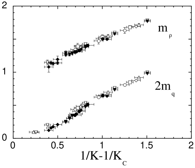
Figure 3: $m_{\rho}a$ and $2m_{q}a$ in the low temperature phase. Open symbols are for $N_{F}=2$, $\beta=3.0$, 3.5, 4.0, 4.3, and 4.5 on an $8^{2}\times 10\times 4$ lattice. Filled symbols are for $N_{F}=3$, $\beta=4.0$, 4.5 and 4.7 on $8^{2}\times 10\times 4$ and $12^{3}\times 4$ lattices. $K_{c}$ for $N_{F}=2$ is used. Horizontal errors are from those of $K_{c}$ with taking into account the difference due to definitions, either the vanishing point of $m_{\pi}^{2}$ or $m_{q}$.

Figure 4: Time history of (a) $N_{\rm inv}$ and (b) the plaquette for $m_{s}\sim 150$ MeV on an $8^{2}\times 10\times 4$ lattice.

Figure 5: Time history of the plaquette for $m_{s}\sim 400$ MeV on a $12^{3}\times 4$ lattice.

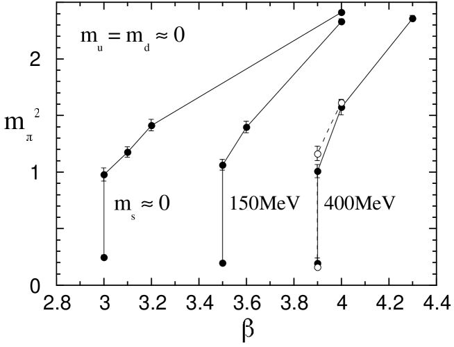
Figure 6: $(m_{\pi}a)^{2}$ versus $\beta$ for $m_{s}\simeq 0$, 150 and 400 MeV with $m_{ud}\simeq 0$. Filled and open symbols are for $8^{2}\times 10\times 4$ and $12^{3}\times 4$ lattices, respectively.

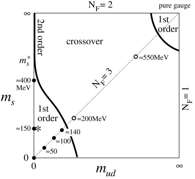
Figure 7: Order of the finite temperature QCD transition in the $(m_{ud},m_{s})$ plane. First order signals are observed at the points marked with filled circle, while no clear two state signals are found at the points with open circle. The values of quark mass in physical units are computed using $a^{-1}\sim 0.8$ GeV. The real world corresponds to the point marked with star. The second order transition line is suggested to deviate from the vertical axis as $m_{ud}\propto(m_{s}^{*}-m_{s})^{5/2}$ below $m_{s}^{*}$.

References

- [1] Y. Iwasaki, K. Kanaya, S. Kaya, S. Sakai and T. Yoshié, Nucl. Phys. B (Proc.Suppl.) 42(1995) 499; Y. Iwasaki, ibid. 96; K. Kanaya, preprint of Tsukuba, UTHEP-296(1994).
- [2] Y. Iwasaki, K. Kanaya, S. Sakai and T. Yoshié, preprint of Tsukuba UTHEP-300(1995).
- [3] For recent review, C. DeTar, preprints of Utah, UU-HEP94/4 and 95/2; F. Karsch, Nucl. Phys. B (Proc. Suppl.) 34(1994) 63.
- [4] R. Pisarski and F. Wilczek, Phys. Rev. D29(1984) 338; F. Wilczek, Int. J. Mod. Phys. A7(1992) 3911; K. Rajagopal and F. Wilczek, Nucl. Phys. B399(1993) 395.
- [5] M. Bochicchio, et al., Nucl. Phys. B262(1985) 331; S. Itoh, Y. Iwasaki, Y. Oyanagi and T. Yoshié, Nucl. Phys. B274(1986) 33.
- [6] R.V. Gavai and F. Karsch, Nucl. Phys. B261(1985) 273; R.V. Gavai, J. Potvin and S. Sanielevici, Phys. Rev. Lett. 58(1987) 2519.
- [7] F.R. Brown, et al., Phys. Rev. Lett. 65(1990) 2491.
- [8] For a review, A. Ukawa, Nucl. Phys. B (Proc. Suppl.) 30(1993) 3.
- [9] K.D. Born, et al., Phys. Rev. D40(1989) 1653.
- [10] Y. Iwasaki, K. Kanaya, S. Sakai and T. Yoshié, Phys. Rev. Lett. 69(1992) 21; S. Itoh, Y. Iwasaki and T. Yoshié, Phys. Rev. D36 (1986) 527.