UTHEP-300

April 1995

Chiral Phase Transition in Lattice QCD with Wilson Quarks

Y. Iwasaki,^a K. Kanaya,^a S. Sakai,^b and T. Yoshié^a

^a Institute of Physics, University of Tsukuba, Ibaraki 305, Japan
^b Faculty of Education, Yamagata University, Yamagata 990, Japan

The nature of the chiral phase transition in lattice QCD is studied for the cases of 2, 3 and 6 flavors with degenerate Wilson quarks, mainly on a lattice with the temporal direction extension $N_{t}=4$. We find that the chiral phase transition is continuous for the case of 2 flavors, while it is of first order for 3 and 6 flavors.

1 Introduction

In this article we investigate the nature of the chiral phase transition in lattice QCD for various numbers of flavors $N_{F}$ in the case of degenerate quarks, taking the Wilson formalism of fermions on the lattice. The determination of the order of the chiral transition, in particular for $N_{F}=2$, is a first step toward the understanding of what happens in the QCD phase transition, which is supposed to occur at the early Universe and possibly at heavy ion collisions. It is also important to compare the results for various number of flavors with theoretical predictions. Because the Wilson formalism of fermions on the lattice is the only known formalism which possesses a local action for any number of flavors, it is urgent to investigate the finite temperature chiral phase transition for various number of flavors with Wilson quarks.

For each $N_{F}$ there are two parameters: $\beta$ ($=6/g^{2}$; g is the gauge coupling constant) and the hopping parameter $K$. Because chiral symmetry is explicitly broken in the Wilson formalism even for a vanishing bare quark mass, we have to begin with the identification of the chiral limit. We define the quark mass through the axial Ward identity[1, 2]

$$2m_{q}<\,0\,|\,P\,|\,\pi\,>=-m_{\pi}<\,0\,|\,A_{4}\,|\,\pi\,>$$

where $P$ is the pseudoscalar density and $A_{4}$ the fourth component of the local axial vector current. At zero temperature the pion mass vanishes at the point which is almost identical to that where the quark mass vanishes[2, 3]. It has been further shown that the value of the quark mass does not depend on whether the system is in the high or the low temperature phase through simulations at $\beta=5.85$ in the quenched QCD [4] and at $\beta=5.5$ for the $N_{F}=2$ case[5]. Therefore we can identify the chiral limit by the vanishing point of the quark mass $m_{q}$. This defines a curve $K_{c}(\beta)$ in the $\beta$ – $K$ plane. Alternatively we may use the vanishing point of $m_{\pi}^{2}$ in the confining phase.

At small $\beta$ region ($\beta\leq 5.0$) where we have made simulations in this work, $m_{q}$ in the deconfining phase does not agree with that in the confining phase and the proportionality between the $m_{q}$ in the deconfining phase and $m_{\pi}^{2}$ in the confining phase is lost, contrary to the situation for $\beta\geq 5.5$ mentioned above. We interpret this as a lattice artifact. On the other hand, the proportionality between the $m_{q}$ in the confining and $m_{\pi}^{2}$ in the confining phase is well satisfied. Therefore we adopt as $K_{c}(\beta)$ the vanishing point of $m_{q}$ in the confining phase $K_{c}(m_{q})$ or that of $m_{\pi}^{2}$ in the confining phase $K_{c}(m_{\pi}^{2})$. The values of $K_{c}(\beta)$ show a slight dependence on the choice of $K_{c}(m_{q})$ or $K_{c}(m_{\pi}^{2})$. They also slightly depend on $N_{F}$ and $N_{t}$. Those at $\beta=4.5$ are listed in Table 1. We find that the difference due to $N_{F}$ is of the same order of magnitude as that due to the difference of definition. The $K_{c}(m_{\pi}^{2})$ for $N_{F}=2$ for various $\beta$’s are listed in Table 2.

The temperature on a lattice is given by $1/N_{t}a$, where $N_{t}$ is the lattice size in the temporal direction and $a$ is the lattice spacing. The location of the transition or crossover $K_{t}(\beta)$ from the high temperature regime to the low temperature regime, for a given $\beta$ and a fixed temporal lattice size $N_{t}$, is identified by a sudden change of physical observables such as the plaquette, the Polyakov line and screening hadron spectrum.

The chiral transition occurs at the crossing point of the $K_{t}(\beta)$ and $K_{c}(\beta)$ line. However, whether the transition $K_{t}$ line with a fixed $N_{t}$ crosses the $K_{c}$ line is not trivial. As was first noticed by Fukugita et al.[6], the $K_{t}$ line creeps deep into the strong coupling region. Therefore before discussing the order of the transition, we have to address ourselves to the problem whether the chiral limit of the finite temperature transition exists at all.

In a previous paper[7] we showed that when $N_{F}\geq 7$, the $K_{t}$ line does not cross the $K_{c}$ line at finite $\beta$. In this article we identify the crossing point for the case $N_{F}\leq 6$ and determine the order of the transition. Preliminary reports are given in [8]. We take the strategy of performing simulations on the line $K_{c}(\beta)$ starting from a $\beta$ in the high temperature phase and reducing $\beta$. We call this method “on-$K_{c}$” simulations. The number of iteration $N_{\rm inv}$ needed for the quark matrix inversion, in general, provides a good indicator to discriminate the high temperature phase from the low temperature phase. The use of $N_{\rm inv}$ as an indicator is extremely useful “on-$K_{c}$”, because $N_{\rm inv}$ is enormously large on the $K_{c}$ line in the confining phase, while it is of order several hundreds in the deconfining phase. This difference is due to the fact that there are zero modes around $K_{c}$ in the low temperature phase, while none exists in the high temperature phase[7, 9]. Therefore there is a sudden drastic change of $N_{\rm inv}$ across the boundary of the two phases. Combining this with measurements of the Polyakov loop, the plaquette and hadron screening masses, we identify the crossing point $\beta_{ct}$ of the $K_{t}(\beta)$ line with the $K_{c}(\beta)$ line. We also check that the crossing point thus determined is consistent with an extrapolation of the line $K_{t}(\beta)$ toward the chiral limit. From the behavior of physical quantities toward $\beta_{ct}$, we are able to determine the order of the chiral transition.

2 Simulations

We mainly perform simulations for the case of $N_{t}=4$ with the spatial size $8^{2}\times 10$. To study the $N_{t}$ dependence for the $N_{F}=2$ case, we also make simulations at $N_{t}=6$ and at $N_{t}=18$ with $12^{3}$ and $18^{2}\times 24$ spatial lattices, respectively. We generate gauge configurations by Hybrid Monte Calro (HMC) algorithm for $N_{F}=2$ with a molecular dynamics step chosen in such a way that the acceptance rate is about 80 – 90%, while for $N_{F}\geq 3$ by the hybrid R algorithm with the molecular dynamics step $\Delta\tau=0.01$, unless otherwise stated. The inversion of the quark matrix is made by a minimal residual method or a conjugate gradient (CG) method. When the hadron spectrum is calculated, the lattice is duplicated in the direction of lattice size 10 or 12. We use an anti-periodic boundary condition for quarks in the $t$ direction and periodic boundary conditions otherwise. The statistics is in general total $\tau=$ several hundreds, and the plaquette and the Polyakov loop are measured every simulation time unit and hadron spectrum is calculated every $\delta\tau=10$ (or less depending on the total statistics). When the value of $\beta$ is small, the fluctuation of physical quantities are small[7] and therefore we think the statistics is sufficient for the purpose of this article.

3 Results

3.1 $N_{F}=2$

Now let us discuss the results for the $N_{F}=2$ case at $N_{t}=4$. The $K_{t}(\beta)$’s obtained by various groups[10, 8] are plotted in Fig. 1 together with the $K_{c}(\beta)$ line[11]. In order to confirm the existence of the crossing point we take the largest (farthest) $K_{c}$, that is $K_{c}(m_{\pi}^{2})$ for $N_{F}=2$ in Table 2 and interpolated ones for “on-$K_{c}$” simulations. We first perform “on-$K_{c}$” simulations by the R algorithm to identify the crossing point, because it is very time consuming due to low acceptance rate for the HMC algorithm on $K_{c}$ in the confining phase. We find that when $\beta\geq 4.0$, $N_{\rm inv}$ stays around several hundreds, while $\beta\leq 3.9$ it increases with $\tau$ and exceeds several thousands (see Fig. 2). Therefore we identify the crossing point at $\beta_{ct}\sim 3.9$ – 4.0. This $\beta_{ct}$ is consistent with a linear extrapolation of the $K_{t}$ line as is shown in Fig. 1. Our results for $K_{t}$ is summarized in Table 3.

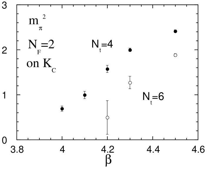
Figure 3: $m_{\pi}^{2}$ for $N_{F}=2$ on $K_{c}$.

Then we repeat “on-$K_{c}$” simulations by the HMC algorithm for $\beta\geq 4.0$ in order to measure physical observables. $N_{\rm inv}$ for $\beta\geq 4.0$ plotted in Fig. 2 is for the HMC algorithm, which is similar to that for the R algorithm. The $\Delta\tau$ toward $\beta_{ct}$ should be taken small in order to keep the acceptance rate reasonably high (for $\beta=4.0$, 4.1 and 4.2 we use $\Delta\tau=0.002$, 0.005 and 0.005 to get acceptance rates 0.91, 0.79 and 0.93, respectively). The value of $m_{\pi}^{2}$ thus obtained decreases toward zero as the chiral transition is approached (see Fig. 3).

We find no two-state signals around $\beta_{ct}$. This is in sharp contrast with the $N_{F}=3$ and 6 cases where we find clear two-state signals at $\beta_{ct}$, as discussed below. This together with the vanishing $m_{\pi}^{2}$ toward $\beta_{ct}$ indicate that the chiral phase transition is continuous for $N_{F}=2$.

The results by “on-$K_{c}$” simulations on the $N_{t}=6$ lattice are similar to those on the $N_{t}=4$ lattice. The estimated transition point is $\beta_{ct}\sim$ 4.0 – 4.2. The value of $m_{\pi}^{2}$ plotted in Fig. 3 again decreases toward zero as $\beta$ approaches $\beta_{ct}$. For $N_{t}=18$ with the spatial size $18^{2}\times 24$, we find that the transition is at $\beta_{ct}\sim 4.5$ – 5.0. Although the spatial size is not large enough, this result suggests that the shift of $\beta_{ct}$ with $N_{t}$ is very slow.

3.2 $N_{F}=3$

Now we perform “on-$K_{c}$” simulations for $N_{F}=3$. In order to confirm the existence of the crossing point we take the largest (farthest) $K_{c}$, that is $K_{c}(m_{\pi}^{2})$ for $N_{F}=2$ at $\beta$’s we have studied, since this is the most stringent condition for the existence of $\beta_{ct}$. We use them and interpolated ones here, and also for $N_{F}=6$ interpolated ones with $K_{c}=0.25$ at $\beta=0$.

Fig. 4 shows $N_{\rm inv}$ as a function of the molecular-dynamics time $\tau$ for several values of $\beta$’s. When $\beta\geq 3.1$, $N_{\rm inv}$ is of order of several hundreds, while when $\beta\leq 2.9$, $N_{\rm inv}$ shows a rapid increase with $\tau$. At $\beta=3.0$ we see a clear two-state signal depending on the initial condition: For a hot start, $N_{\rm inv}$ is quite stable around $\sim 800$ and $m_{\pi}^{2}$ is large ($\sim 1.0$). On the other hand, for a mix start, $N_{\rm inv}$ shows a rapid increase with $\tau$ and exceeds 2,000 in $\tau\sim 20$, and in accord with this, $m_{\pi}^{2}$ decreases with $\tau$.

The value of $m_{\pi}^{2}$ is plotted in Fig. 5. At $\beta=3.0$ we have two values for $m_{\pi}^{2}$ depending on the initial configuration. The larger one obtained for the hot start is of order 1.0, which is a smooth extrapolation of the values at $\beta\sim 3.1$ - 3.2. The smaller one is an upper bound for $m_{\pi}^{2}$ for the mix start.

We note that the result of $\beta_{ct}\sim 3.0$ is consistent with an extrapolation of $K_{t}$ points listed in Table 3 as is shown in Fig. 1. Thus we identify the crossing point at $\beta_{ct}\sim 3.0(1)$. With the clear two-state signal we conclude that the chiral transition is of first order for $N_{F}=3$.

3.3 $N_{F}$ = 6

Finally let us discuss the results for $N_{F}=6$. Our previous study[7] implies that this number of flavor is critical for the existence of the crossing point and therefore it is important to establish the existence of the crossing in this case. Overall features of the transition for $N_{F}=6$ are very similar to those for $N_{F}=3$ except for the position of $\beta_{ct}$, which moves to a smaller $\beta$ as expected. Fig. 6 shows that $N_{\rm inv}$ “on-$K_{c}$” stays at several hundreds for $\beta\geq 0.4$ and for a hot start at $\beta=0.3$. On the other hand, $N_{\rm inv}$ grows rapidly with $\tau$ and exceeds 5,000 for $\beta\leq 0.2$ and for a mix start at $\beta=0.3$. In accord with this, we have two values of $m_{\pi}^{2}$ at $\beta=0.3$ (Fig. 7). Therefore we identify the crossing point at $\beta_{ct}\sim 0.3(1)$ and conclude that the chiral transition is of first order for $N_{F}=6$. This $\beta_{ct}$ is consistent with a linear extrapolation of the $K_{t}$ line ($K_{t}=0.245$ – 0.2475, 0.235 – 0.237, and 0.166 – 0.168 for $\beta=0.5$, 1.0, and 4.5, respectively).

4 Conclusions

It should be noted that our main results obtained in this work that the chiral transitions for $N_{F}=3$ and 6 are of first order, while it is continuous for $N_{F}=2$, are consistent with the prediction based on universality[12]. Our results with Wilson fermions are also consistent with those with staggered fermions[13].

The simulations on the $N_{t}=4$ and 6 lattices and the $N_{t}=18$ lattice have been performed with HITAC S820/80 at KEK and with QCDPAX at the University of Tsukuba, respectively. We would like to thank members of KEK for their hospitality and strong support and the other members of QCDPAX collaboration for their help. This project is in part supported by the Grant-in-Aid of Ministry of Education, Science and Culture (No.62060001 and No.02402003).

	$N_{t}=4$		$N_{t}=8$
$N_{F}$	$K_{c}(m_{\pi}^{2})$	$K_{c}(m_{q})$	$K_{c}(m_{\pi}^{2})$	$K_{c}(m_{q})$
2	0.214(1)	0.210(1)	0.212(1)	0.209(1)
3	0.209(1)	0.204(1)
6	0.205(2)	0.200(1)

Table 1: Chiral limit $K_{c}$ at $\beta=4.5$ determined by vanishing $m_{\pi}^{2}$ and $m_{q}$. Values of $m_{\pi}^{2}$ and $m_{q}$ in the confinig phase are linearly extrapolated in $1/K$ using data from $K=0.16$ – 0.18 for $N_{F}=2$ and 3 and $K=0.15$ – 0.165 for $N_{F}=6$ (because $K_{t}=0.167(1)$ for $N_{F}=6$ at $N_{t}=4$). The spatial lattice size is $8^{2}\times 10$.

$\beta$	3.0	3.5	4.0	4.3
$K_{c}(m_{\pi}^{2})$	0.235(1)	0.230(1)	0.223(1)	0.218(1)
$K_{c}(m_{q})$	0.230(1)	0.226(1)	0.218(4)	0.214(1)

Table 2: $K_{c}$ for $N_{F}=2$ determined on an $8^{2}\times 10\times 4$ lattice. The results for $\beta=4.5$ are given in Table 1.

$N_{F}=2$		$N_{F}=3$
$\beta$	$K_{t}$	$\beta$	$K_{t}$
4.3	0.207 – 0.210	3.0	$>$ 0.230
4.5	0.200 – 0.202	4.0	0.200 – 0.205
5.0	0.170 – 0.180	4.5	0.186 – 0.189
5.25	0.160 – 0.165	4.5*	0.186 – 0.189
		4.7*	0.179 – 0.180
		5.0	0.166 – 0.1665
		5.5	0.1275 – 0.130

Table 3: Finite temperature transition/crossover $K_{t}$ for $N_{F}=2$ and 3 obtained on an $8^{2}\times 10\times 4$ lattice (data with * obtained on a $12^{3}\times 4$ lattice).

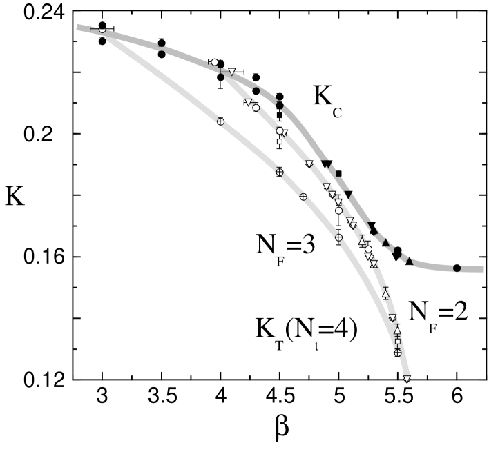
Figure 1: Phase diagram for $N_{F}=2$ and 3. Filled symbols are for $K_{c}(m_{\pi}^{2})$ and $K_{c}(m_{q})$. Open symbols are for $K_{t}(N_{t}=4)$ for $N_{F}=2$ while open circles with cross for $N_{F}=3$. Circles are our data. Lines are for guiding eyes.

Figure 2: Molecular-dynamics time history of $N_{\rm inv}$ for $N_{F}=2$ on $K_{c}$.

Figure 4: Time history of $N_{\rm inv}$ for $N_{F}=3$ on $K_{c}$.

Figure 5: $m_{\pi}^{2}$ for $N_{F}=3$ on $K_{c}$.

Figure 6: Time history of $N_{\rm inv}$ for $N_{F}=6$ on $K_{c}$.

Figure 7: $m_{\pi}^{2}$ for $N_{F}=6$ on $K_{c}$.

References

- [1] M. Bochicchio et al., Nucl. Phys. B262 (1985) 331.
- [2] S. Itoh, Y. Iwasaki, Y. Oyanagi and T. Yoshié, Nucl. Phys. B274(1986) 33.
- [3] L. Maiani and G. Martinelli, Phys. Lett. 178B (1986) 265.
- [4] Y. Iwasaki, T. Tsuboi and T. Yoshié, Phys. Lett. B220 (1989) 602.
- [5] Y. Iwasaki, K. Kanaya, S. Sakai and T. Yoshié, Phys. Rev. Lett. 67 (1991) 1494.
- [6] M. Fukugita, S. Ohta and A. Ukawa, Phys. Rev. Lett. 57 (1986) 1974.
- [7] Y. Iwasaki, K. Kanaya, S. Sakai and T. Yoshié, Phys. Rev. Lett. 69 (1992) 21.
- [8] Y. Iwasaki, K. Kanaya, S. Sakai and T. Yoshié, Nucl. Phys. B (Proc. Suppl.) 30 (1993) 327; ibid. 34 (1994) 314.
- [9] S. Itoh, Y. Iwasaki and T. Yoshié, Phys. Rev. D36(1986) 527.
- [10] R. Gupta et al., Phys. Rev. D40 (1989) 2072; A. Ukawa, Nucl. Phys. B (Proc. Suppl.) 9 (1989) 463; K. Bitar et al., Phys. Lett. B234 (1990) 333; Phys. Rev. D43 (1991) 2396; C. Bernard et al., ibid. D46 (1992) 4741; ibid. D49 (1994) 3574; Nucl. Phys. B (Proc. Suppl.) 34 (1994) 324; T. Blum et al., Phys. Rev. D50 (1994) 3377.
- [11] See references in Y. Iwasaki, preprint of Tsukuba UTHEP-293(1994).
- [12] R. Pisarski and F. Wilczek, Phys. Rev. D29 (1984) 338; F. Wilczek, Int. J. Mod. Phys. A7 (1992) 3911; K. Rajagopal and F. Wilczek, Nucl. Phys. B399 (1993) 395.
- [13] For recent review, C. DeTar, preprint of Utah, UU-HEP94/4; F. Karsch, Nucl. Phys. B (Proc. Suppl.) 34 (1994) 63.