SU-4240-607

Scaling and the Fractal Geometry
of Two-Dimensional Quantum Gravity

S. Catterall
G. Thorleifsson
M. Bowick
V. John
Physics Department, Syracuse University,

Syracuse, NY 13244.

We examine the scaling of geodesic correlation functions in two-dimensional gravity and in spin systems coupled to gravity. The numerical data support the scaling hypothesis and indicate that the quantum geometry develops a non-perturbative length scale. The existence of this length scale allows us to extract a Hausdorff dimension. In the case of pure gravity we find $d_{H}\approx 3.8$, in support of recent theoretical calculations that $d_{H}=4$. We also discuss the back-reaction of matter on the geometry.

1 Introduction

Remarkable strides have been made in recent years in our understanding of the properties of two-dimensional quantum gravity [1]. Calculations carried out within the framework of conformal field theory have yielded the gravitational dressing of integrated matter field operators, correlation functions on the sphere and the torus partition function. On the other hand matrix models have provided us with a powerful calculational tool that enables us to compute the above mentioned quantities and also to perform the non-perturbative sum over topologies.

Nevertheless there are still important geometrical quantities of physical interest that are not well understood analytically. Perhaps the most fundamental is the intrinsic Hausdorff dimension of the typical surface generated by the coupling of matter to $2d$-gravity [2, 3]. One may think of the Hausdorff dimension as an order parameter characterizing possible phases of the theory. If there exists a power law relation between two reparametrization invariant quantities with the dimension of volume ($V$) and length ($L$), this provides a well-defined fractal dimension ($d_{H}$) via $V\propto L^{d_{H}}$. As there is no natural notion of a length scale in these theories, one has to be introduced by hand, at least in the continuum formulation. In the discretized approach this length scale is provided by the short distance cut-off corresponding to the finite elementary link length.

Recently a transfer matrix formalism utilizing matrix model amplitudes has been developed that predicts the Hausdorff dimension $d_{H}=4$ for pure $2d$ gravity [4]. This approach has not yet been extended to the case of unitary minimal models coupled to gravity. On the other hand the analysis of the diffusion equation for a random walk on the ensemble of $2d$ manifolds determined by the Liouville action yields a prediction for the Hausdorff dimension which agrees with the transfer matrix approach for pure gravity. It may also be extended to include the coupling of conformal matter of central charge $c\leq 1$ [5].

These analytic predictions for the Hausdorff dimension rely on the validity of certain scaling assumptions. It also appears that there are several potentially inequivalent definitions of an appropriate fractal dimensionality. It seems very worthwhile therefore to explore these issues numerically. Earlier numerical work addressing this question has been remarkably inconclusive [6, 7, 8]. Indeed for a while it was claimed that there was no well-defined Hausdorff dimension in the case of pure gravity [7]. In contrast clear numerical evidence for a fractal scaling of gravity coupled to $c=-2$ matter was found in [9].

In this letter we establish numerically that this scaling behavior is valid for pure gravity as well as the Ising and 3-state Potts models coupled to gravity. We employ a careful finite size scaling analysis of appropriate correlation functions. For pure gravity we find $d_{H}\approx 3.8$ in qualitative agreement with [3, 4, 5]. For the Ising and 3-state Potts models the values of $d_{H}$ that we obtain do not seem to detect the back reaction of matter on the geometry.

This paper is organized as follows. In section 2 we describe the application of finite size scaling to loop-loop correlation functions. In section 3 we outline our numerical procedures and results. In section 4 we present the existing theoretical predictions for the Hausdorff dimension. Finally section 5 is a discussion of our conclusions.

2 Scaling

Finite size scaling is a well-established technique for analyzing the critical behavior of conventional statistical mechanical models [10]. In numerical studies of quantum gravity it has traditionally been employed in a rather limited context - typically by extracting a power law scaling for integrated matter field operators at the critical point.

In general, the scaling hypothesis asserts that near a critical point an observable $O$, a function of two variables $x$ and $y$, will depend on only one scaling combination $\mu=y/x^{q}$ up to an overall power factor $x^{p}$

$$O\left(x,y\right)\sim x^{p}f\left(y/x^{q}\right).$$ (1)

The powers $p$ and $q$ are related to the critical exponents of the model. We will test this hypothesis by analyzing geodesic correlators defined on dynamical triangulations.

The fundamental objects in two-dimensional gravity are loop-loop correlators. To define these consider two marked loops of length $l$ and $l^{\prime}$ on a triangulation. If we define a geodesic distance $r$ between the loops on the graph as the minimal number of links that must be traversed to go from $l$ to $l^{\prime}$, we can define a correlation function $n_{l,l^{\prime}}\left(r\right)$ as

$$n_{l,l^{\prime}}(r,N)=\sum_{T\in{\cal T}_{2}(N)}1\;.$$ (2)

In this expression ${\cal T}_{2}(N)$ refers to the class of triangulations with $N$ triangles and two loops of length $l$ and $l^{\prime}$ separated by a geodesic distance $r$. As defined above $n_{l,l^{\prime}}(r,N)$ is proportional to the number of triangulations satisfying the above constraints. We chose to work in the microcanonical ensemble as it is convenient computationally and the effect of restricting to fixed volume can be exploited in the finite size scaling analysis. The point-point correlator $n(r,N)$, which counts the number of triangulations with two marked points separated by geodesic distance $r$, can now be obtained from Eq. (2) in the limit that the lengths of the loops are taken to zero.

The scaling hypothesis applied to $n\left(r,N\right)$ implies

$$n\left(r,N\right)=N^{p}\;n\left(r/N^{q}\right)\;.$$ (3)

The combination $l_{G}=N^{q}$ constitutes a dynamical length scale which appears non-perturbatively in the theory. It can be used to define a Hausdorff or fractal dimension $d_{H}=1/q$ characterizing the quantum geometry. Notice that in this case the exponent $p$ is not free ${-}$ it is constrained by the fact that the integral of $n\left(r,N\right)$ over all geodesic distances recovers the total number of points $N$. This yields $p=1-1/d_{H}$. It is easy to measure the point-point correlator numerically and thus determine $d_{H}$.

This discussion can be generalized to include spin models coupled to gravity. In this case the boundary loops will be dressed with fixed boundary spin configurations. For the point-point correlator we can use the symmetry of the spin models to reduce the possible correlators to two distinct types, which we denote $f_{1}\left(r,N\right)$ and $f_{2}\left(r,N\right)$. The correlator $f_{1}$ counts the number of points at distance $r$ for which the spin variable is in the same state as the initial marked point. The correlator $f_{2}$ counts the number of spins in a different state from the initial marked point. The total number of points at geodesic distance $r$ is then

$$n\left(r,N\right)=f_{1}\left(r,N\right)+f_{2}\left(r,N\right).$$ (4)

The scaling hypothesis can be applied as before to these correlators, resulting in a definition of $d_{H}$.

To define spin-spin correlators we note that the spin variables of the $q$-state Potts model may be taken to be the unit vectors $\vec{e}_{\alpha}$ of a hyper-tetrahedron in $q-1$ dimensional space. We can then identify the product of two spins as the scalar product of the associated link vectors

$$\sigma_{\alpha}\sigma_{\beta}\equiv\vec{e}_{\alpha}\cdot\vec{e}_{\beta}=\left(1+\frac{1}{q-1}\right)\delta_{\alpha\beta}-\frac{1}{q-1}.$$ (5)

The (unnormalized) spin-spin correlator with one marked point $i$ is

$$g_{un}(r,N)=\sum_{T}\sum_{\{\sigma_{i}\}}\sum_{j}\sigma_{i}\sigma_{j}\;\delta(d_{ij}-r)\;e^{{\textstyle-S_{N}(\sigma,T)}}\;\;.$$ (6)

In terms of the distributions $f_{1}$ and $f_{2}$ defined earlier we see from Eq. (5) that this may be written as

$$g_{un}(r,N)=f_{1}\left(r,N\right)-{1\over q-1}f_{2}\left(r,N\right).$$ (7)

The scaling hypothesis for $g_{un}$ takes the form

$$g_{un}(r,N)=N^{\frac{\gamma}{\nu d_{H}}-s}g_{un}(r/N^{s}).$$ (8)

The overall power is again determined from the constraint that the integral of $g_{un}(r,N)$ is just the usual magnetic susceptibility, which scales at criticality as $\chi\sim N^{{\gamma\over\nu d_{H}}}$. If we make the assumption that these critical systems contain only one length scale then it is natural to assume that both $n(r,N)$ and $g_{un}(r,N)$ depend on the same scaling variable. This implies that $s=1/d_{H}$, where the Hausdorff dimension $d_{H}$ is now that appropriate to the matter-coupled theory. We shall re-examine this assumption critically in light of the numerical results in the final section of the paper.

We will also consider the normalized spin-spin correlator with one marked point $i$:

$$g_{n}(r,N)=\sum_{T}\frac{1}{\sum_{j}\delta(d_{ij}-r)}\sum_{\{\sigma_{i}\}}\sum_{j}\sigma_{i}\sigma_{j}\;\delta(d_{ij}-r)\;e^{{\textstyle-S_{N}(\sigma,T)}}\;\;.$$ (9)

3 Numerical Simulations

To investigate the validity of the scaling hypothesis we have performed Monte Carlo simulations on three models; pure gravity (central charge $c=0$), the Ising model $(c=1/2)$ and 3-state Potts model $(c=4/5)$ coupled to gravity. In the microcanonical ensemble the partition function of these models is given by

$$Z(\beta,N)=\sum_{T\in{\cal T}}Z_{M}(\beta,N)$$ (10)

where $Z_{M}(N,\beta)$ describes the matter sector (absent for pure gravity). For a $q$-state Potts model this is

$$Z_{M}(\beta,N)=\sum_{\{\sigma_{i}\}}{\rm exp}\left(\beta\sum_{<i,j>}(\delta_{\sigma_{i},\sigma_{j}}-1)\right),$$ (11)

were $\sigma_{i}$ denote the Potts spins, $i$ denotes a lattice site and $<i,j>$ indicates that the sum is over nearest- neighbor pairs on the lattice.

The integration over manifolds is implemented as a sum over an appropriate class of triangulations ${\cal T}$. Since it has been observed that finite size effects in numerical determinations of critical exponents are generally smaller if one includes degenerate triangulations in ${\cal T}$, i.e. triangulations allowing two vertices connected by more than one link and vertices connected to itself [11], we will work in that ensemble.

In the simulations a standard link-flip algorithm was used to explore the space of triangulations and a Swendsen-Wang cluster algorithm employed for the spin updates. Lattice sizes ranging from 500 to 32000 triangles were studied and typically $10^{6}$ to $4\times 10^{6}$ Monte Carlo sweeps performed for each lattice size (a sweep consists of flipping about $N$ links and one SW update of the spin configuration).

3.1 Pure Gravity

We start with the results for pure gravity. Here we measured the point-point distributions $n(r,N)$ both on the direct and the dual lattice. On the dual lattice geodesic distances are measured as shortest paths going from one vertex to another. Having measured these distributions for different lattice sizes there are several ways we can use the scaling assumption Eq. (3) to extract $d_{H}$. We use two methods.

First we fitted a distribution (for a given lattice size) to an appropriately chosen function from which we located the maximum of the distribution $r_{0}$ and its maximal value $n(r_{0})$. Then the scaling assumption implies that $r_{0}\sim N^{1/d_{H}}$ and $n(r_{0})\sim N^{1-1/d_{H}}$. We fit to the function

$$P_{l}(r)\>{\rm exp}(-ar^{b})\;.$$ (12)

The exponential is included in order to capture the long-distance behavior of the distribution and $P_{l}$ is an $l$-order polynomial. The order of the polynomial is chosen in such way that we get a reasonably good fit; a 4th order polynomial turned out to be sufficient. We checked that the values of $r_{0}$ and $n(r_{0})$ did not change appreciably if we increased the order of $P_{l}(r)$. The values of $r_{0}$ and $n(r_{0})$ obtained in this way are plotted in Figs. 1a and 1b on log-log plots. As expected both quantities scale well with $N$ (significantly better for the direct lattice). The Hausdorff dimensions extracted from the slopes are listed in Table 1.

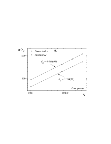
Figure 1: Volume scaling of (${\it a}$) the location of the peak $r_{0}$ in the distributions $n(r,N)$ and (b) their maximal value $n(r_{0})$ in the case of pure gravity. Data is shown both for the direct and dual lattices and the extracted values of $d_{H}$ are included.

	Direct lattice		Dual lattice
	$d_{H}$	$\tilde{\chi}^{2}$	$d_{H}$	$\tilde{\chi}^{2}$
(a)
$126-250$	3.640(60)	44.6	2.497(37)	49.2
$250-500$	3.707(45)	13.0	2.715(40)	29.1
$500-1000$	3.727(42)	8.0	2.871(38)	20.5
$1000-2000$	3.770(38)	4.2	2.996(26)	22.6
$2000-4000$	3.800(54)	2.3	3.111(39)	12.5
$4000-8000$	3.804(55)	1.5	3.217(47)	9.7
$8000-16000$	3.810(55)	0.97	3.264(34)	6.9
$16000-32000$	3.830(50)	1.4	3.411(89)	4.8
(b)
$1000-32000$	3.790(30)	13.0	3.150(31)	85
(c)
position	$3.835(59)$	0.03	$3.133(43)$	10.45
height	$4.040(98)$	0.09	$3.594(77)$	0.37

Table 1: Extracted values of $d_{H}$ from $n(r,N)$ in the case of pure gravity. The values in (a) are obtained by collapsing data for two consecutive lattices sizes on a single curve using one scaling parameter. (b) is the same except data from all lattice sizes between 1000 and 32000 triangles are used. In (c) the values are obtained from the volume scaling of $r_{0}$ and $n(r_{0})$ separately. The quality of the fit is indicated by $\tilde{\chi}^{2}$ and the errors in (a) and (b) indicate where $\tilde{\chi}^{2}$ changes by one unit from its minimal value.

Another way to extract $d_{H}$ is to use the scaling relations directly to collapse distributions for different lattices sizes on to the same curve, using only a single scaling parameter $d_{H}$. This we have done including all the data (for $N\geq 1000$) and also, to explore the finite size corrections, using only pairs of datasets ($N$ and $2N$). The same functional form Eq. (12) was used in the fits. The results are shown in Table 1, together with the quality of the fits ($\tilde{\chi}^{2}=\chi^{2}/{\it dof}$). The errors quoted indicate where $\tilde{\chi}^{2}$ changes by one unit from its minimal value. In Figs. 2a and 2b we show overall scaling plots for $n(r,N)$, both for the direct and dual lattices.

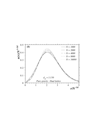
Figure 2: Scaling plots for the point-point distributions $n(r,N)$ in the case of pure gravity; (a) the direct and (b) dual lattice. Shown are the curves fitted to distributions after rescaling. The value of $d_{H}$ is chosen so as it minimized the total chi-square of the fits.

From these results we can immediately draw a number of conclusions. Consider first the direct lattice. Fig. 2a shows that the scaling hypothesis is indeed well satisfied for the distribution $n(r,N)$. This is also evident from the low values of $\tilde{\chi}^{2}$ for the fits (Table 1). The values of $d_{H}$ obtained from the scaling of $r_{0}$ and $n(r_{0})$ and also from collapsing the data are close to the expected value of $d_{H}=4$. These results are obtained on moderately small lattices, illustrating the superiority of this method of extracting $d_{H}$ to earlier numerical attempts.

But we also notice that there is a systematic increase in the value of $d_{H}$ with lattice size. Even though this effect is too small compared to the uncertainty in the measured values to allow reliable extrapolation to infinite volume $d_{H}$, it indicates that the difference between measured and expected values of $d_{H}$ is due to finite-size effects. The improvement of the $\tilde{\chi}^{2}$ values of the fits with increasing lattice size also implies diminishing deviations from scaling.

It is also intriguing that the scaling of the peak heights seems to give better values of $d_{H}$ (close to the theoretical results for the direct lattice). Since the heights of the peaks take continuous values, as opposed to the discrete geodesic distance, it plausible that they are less sensitive to the discretization

On the dual lattice we observe much larger finite size deviations. This is evident both from Fig. 2b and the values of $\tilde{\chi}^{2}$ in Table 1. This is not hard to understand. The short distance behavior of $n(r,N)$ is dominated by a power growth $r^{d_{H}-1}$. But as the order of vertices on the dual lattice is fixed to be three, the growth of $n(r,N)$ is bounded by the function $3\times 2^{r-1}$. If $d_{H}=4$ this means that for small values of $r$ the distribution $n(r,N)$ may not grow fast enough to display the correct fractal structure. Only when the lattices are big enough so that the first few steps are negligible can the dual lattice be used to extract $d_{H}$. This constraint on the growth is not present on the direct lattice, which is thus better suited for extracting $d_{H}$.

3.2 Coupling to matter

To see how the point-point distributions (and $d_{H}$) change as we include coupling to matter we looked at both the Ising and 3-state Potts models coupled to gravity. These models are chosen because in both cases the exact solution of the models is known; knowing the exact critical coupling makes the simulations much easier.

	Ising model		3-state Potts model
Exponent	Measured	Exact	Measured	Exact
$\beta/\nu d_{H}$	0.167(3)	1/6	0.199(4)	1/5
$\gamma/\nu d_{H}$	0.653(8)	2/3	0.608(6)	3/5
$1/\nu d_{H}$	0.318(12)	1/3	0.382(30)	2/5

Table 2: Comparing critical exponents, obtained using finite sizes scaling in $\beta_{c}$, to exact values, for the Ising and 3-state Potts models coupled to gravity

As shown in the case of pure gravity it is preferable to measure on the direct lattice and so we have placed the spins on the vertices. In that case the critical couplings are (as we include degenerate triangulations):

$$\beta_{c}=\frac{1}{2}\log\left[\frac{13+\sqrt{7}}{14-\sqrt{7}}\right]\;({\rm Ising})\;\;\;{\rm and}\;\;\;\beta_{c}=\frac{1}{2}\log\left[\frac{41+\sqrt{47}}{47-2\sqrt{47}}\right]\;({\rm 3-state\;Potts}).$$ (13)

To verify that these are indeed the correct couplings we have performed a standard finite size scaling analysis of some observables related to the spin models; the average magnetization ${\cal M}\sim N^{-\beta/\nu d_{H}}$, the magnetic susceptibility $\chi\sim N^{\gamma/\nu d_{H}}$, and the derivative of Binders cumulant $\partial BC/\partial\beta\sim N^{1/\nu d_{H}}$. The measured critical exponents are shown in Table 2, together with the exact values with which they agree very well. The main reason is, of course, that we know $\beta_{c}$, but also including degenerate triangulations and placing the spins on vertices reduces finite-size effects dramatically.

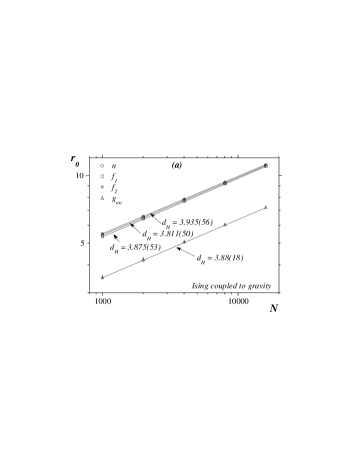
Figure 3: Volume scaling for $r_{0}$ and $n(r_{0})$ for the distributions we measured for Ising model coupled to gravity. The same scaling behavior is used to extract $d_{H}$ from the slope as in the case of pure gravity, except for $g_{un}(r_{0})$. There we used $n(r_{0})\sim\gamma/\nu d_{H}-1/d_{H}$, substituting the exact values for $\gamma/\nu d_{H}$.

Now to the distribution functions. The placement of spins on the vertices allows us to measure several combinations of distributions; $f_{1}(r,N)$, $f_{2}(r,N)$, $n(r,N)$ and $g_{un}(r,N)$. We have analyzed these distributions in the same way as for pure gravity. In Figs. 3a and b we show the scaling with volume of $r_{0}$ and $n(r_{0})$, obtained from fitting the distributions to the functional form Eq. (12). These plots are for the Ising model but plots for the 3-state Potts model are very similar. The extracted Hausdorff dimensions, for $n(r,N)$ and $g_{un}(r,N)$, are shown in Table 3. As for pure gravity we also scaled all the data (for $N\geq 1000$), and for pairs of distributions, on a single curve. Resulting optimal values of $d_{H}$ are listed in Table 3. The quality of the scaling is shown in Figs. 4a and b, where we show scaling plots for $n(r,N)$ and $g_{un}(r,N)$ (for the Ising model). Again the value of $d_{H}$ that minimizes $\tilde{\chi}^{2}$ is used to scale the data.

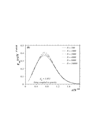
Figure 4: Collapsing the data for $n(r,N)$ and $g_{un}(r,N)$ on a single curve using one scaling parameter in the case of an Ising model coupled to gravity.

In the case of the spin models we also measured the normalized spin-spin correlation function $g_{n}(r,N)$. At the critical point $g_{n}(r,N)$ is expected to have the following behavior

$$g_{n}(r,N)\sim\frac{e^{\textstyle-m(N)\;r}}{r^{\eta}}\;\;,$$ (14)

were the mass gap $m(N)$ vanishes in the infinite volume limit. Surprisingly we only see the exponential decay of the spin-spin correlator and not the power fall-off underneath it (on a log plot we have a straight line for some range of $r$). If we assume that the inverse mass gap is yet another measure of a characteristic length scale for the system, the observed power law dependence is an alternative measure of the Hausdorff dimension.

Looking at the data it is clear that the scaling hypothesis is satisfied as well here as for pure gravity. What is surprising is that the extracted values of $d_{H}$, with two exceptions, are almost the same as for pure gravity. The exceptions, for both models, are the scaling of the peak height of $g_{un}(r,N)$ and $d_{H}$ obtained from the mass gap, both indicating larger values of $d_{H}$. Why is it that we do not seem to see any effects of the back reaction of matter on the fractal dimension?

A possible explanation would be that the critical region is slightly shifted away from the infinite volume critical coupling at the finite volumes we simulate. This is, for example, observed in measurements of the string susceptibility [13], where measured values of $\gamma_{s}$ peak away from $\beta_{c}$. To check this we have measured $d_{H}$ for the Ising model over an interval of $\beta$. Within errors the extracted value of $d_{H}$ did not change over this interval.

In the case of pure gravity we see that the scaling of the peak height gives better results. If we believe this we get different values for $d_{H}$ depending on which point-point correlator we examine. Looking at $n(r,N)$ we get $d_{H}\approx 3.9$ for both models, and observe no back reaction from the matter. The distribution $g_{un}(r,N)$, on the other hand, indicates $d_{H}>4$, and indeed gives results that might be consistent with the values predicted in [5]. This is supported by the scaling of the mass gap of the spin-spin correlator. We will return to this in the discussion section.

	Ising model				3-state Potts model
	$n(r,N)$		$g_{un}(r,N)$		$n(r,N)$		$g_{un}(r,N)$
	$d_{H}$	$\tilde{\chi}^{2}$	$d_{H}$	$\tilde{\chi}^{2}$	$d_{H}$	$\tilde{\chi}^{2}$	$d_{H}$	$\tilde{\chi}^{2}$
(a)
500-1000	3.758(53)	2.6	3.76(12)	0.93	3.752(63)	0.68	4.01(26)	2.5
1000-2000	3.802(55)	0.77	3.75(15)	1.0	3.787(65)	0.29	4.11(18)	1.0
2000-4000	3.833(56)	1.0	3.73(12)	2.5	3.864(63)	1.0	4.04(22)	3.2
4000-8000	3.893(61)	0.88	3.69(09)	3.9	3.870(73)	0.15	4.11(19)	0.41
8000-16000	3.870(87)	0.35	3.80(10)	0.99	3.820(97)	0.58	4.14(15)	0.56
(b)
1000-16000	3.862(74)	1.4	3.851(53)	4.5	3.831(32)	2.4	3.966(64)	12.5
(c)
position	3.875(53)		3.88(19)		3.879(29)		4.141(58)
height	4.01(15)		4.36(18)		3.900(41)		4.424(35))
mass gap	4.51(20)				4.56(43)

Table 3: Extracted values of $d_{H}$ for the Ising and 3-state Potts models coupled to gravity. The values are obtained in the same way as for pure gravity (Table 1).

4 Hausdorff Dimension - Analytic results

In this section we briefly review the continuum and matrix model derivations of the intrinsic Hausdorff dimension ($d_{H}$) of the surfaces generated by the coupling of $2d$ gravity to matter [3, 4, 5, 14]. There are several potentially inequivalent ways to define an appropriate measure of the fractal dimensionality of random surfaces. In the original paper of [14] two methods were proposed. In the first method one determines a power-like relation between two gauge-invariant observables with dimensions of volume ($V$) and length ($L$) respectively, with $d_{H}$ determined by $V\propto L^{d_{H}}$. The volume is measured by the cosmological term and the length by the anomalous dimension of a test fermion which couples to the gravitational field but generates no back reaction. This yields

$$d_{H}=2{\sqrt{25-c}+\sqrt{13-c}\over\sqrt{25-c}+\sqrt{1-c}}\;.$$ (15)

In the second method one considers the diffusion of a test fermion field and determines $d_{H}$ by the short-time come-back probability $p(\tau)\propto\tau^{-d_{H}/2}$. The authors were able to determine the Hausdorff dimension in a double power series expansion in $\epsilon=D-2$ and ${-1\over c}$, where $D$ is the classical dimensionality of the surface and $c$ is the central charge of the matter coupled to gravity. In [5] this second method was applied instead to a scalar field – one considers the diffusion equation for a random walk on the ensemble of $2d$ manifolds determined by the Liouville action. This yields

$$d_{H}=-2{\alpha_{1}\over\alpha_{-1}}=2{\sqrt{25-c}+\sqrt{49-c}\over\sqrt{25-c}+\sqrt{1-c}}\;,$$ (16)

where $e^{\alpha_{1}\phi}$ corresponds to the cosmological constant operator, which has dimension one, and $e^{\alpha_{-1}\phi}$ corresponds to the Liouville dressing of the Laplacian, which requires it to be of conformal dimension $-1$.

In the matrix-model/dynamical triangulation approach the transfer matrix formulation can be used to obtain an expression for the Hausdorff dimension in the case of pure gravity [3, 4]. One finds $d_{H}=4$ in agreement with Eq. (16) for $c=0$.

For the case of pure gravity this result can be compared with [4]. Using matrix model results it is possible to show that

$$\rho(L;D)={3\over 7\sqrt{\pi}}{1\over D^{2}}\left(x^{-5/2}+{1\over 2}x^{-3/2}+{14\over 3}x^{-1/2}\right)e^{-x},$$ (17)

where $\rho(L;D)$ is the number of boundaries separated by geodesic distance $D$ from a loop of length $L$ with one marked point, and the scaling variable $x={L\over D^{2}}$. Now one can consider the quantities $<L^{n}>=\int_{a}^{\infty}dLL^{n}\rho(L;D)$, where $a$ is the lattice constant. From Eq. (17) it can be shown that:

$$<L^{0}> \simeq const\times D^{3}a^{-3/2}+constDa^{-1/2}+constD^{0}$$ (18)

$$<L^{1}> \simeq const\times D^{3}a^{-1/2}+constD^{2}$$ (19)

$$<L^{n}> \simeq const\times D^{2n}\;\;\;(n\geq 2).$$ (20)

Then, using the definition $\langle L^{0}\rangle\propto r^{d_{H}-1}$, one can read off the Hausdorff dimension $d_{H}=4$, which agrees with the continuum result and our numerical results based on scaling arguments. This result is not universal because of the explicit lattice dependence in $<L^{0}>$. One obtains the same result, however, from the second and higher moments provided one assumes that $<L^{2}>$ scales like the area $A$. The result thus appears to be universal.

The general situation is, however, far from clear. One case where there is an obvious discrepancy seems to be the $(2,2k-1)$ series of minimal models coupled to gravity. It is possible to extend the continuum Liouville theory analysis to these models after taking into account the fact that these non-unitary models possess operators in the matter sector with negative conformal dimensions. It is also possible to use the results obtained in [15] to calculate the Hausdorff dimensions for models (with ‘$k$’ even). We find that the results thus obtained do not agree with each other except for the cases $k=1,2$.

The expression for the distribution of loops at a geodesic distance ‘D’ for the $(2,2k-1)$ models coupled to gravity (for even ‘$k$’) was computed in [15]. They find that

$$\rho(L;D)\simeq{1\over D^{1\over\sigma}}\left[{\gamma_{1}\over\gamma_{2}\Gamma(\sigma)}x^{-\sigma-2}(2\sigma+1+x)+{x^{\sigma}\over\Gamma(\sigma+1)}\right]e^{-x},$$ (21)

where $\sigma=k-3/2$ and $\gamma_{1},\gamma_{2}$ are ‘$k$’ dependent constants. Using the same arguments as in the case of pure gravity we can compute $d_{H}=(2k-1)/(2k-3)+1$.

The continuum result of Kawamoto can also be extended to this case, with the difference being that the cosmological constant is not the dressing of the identity operator but of the operator with the lowest conformal dimension. Similarly the dressing condition for the Laplacian is that the Liouville field has dimension $-1-\Delta_{min}$.

Then one obtains:

$$\alpha_{+} = {-k\over\sqrt{2k-1}}$$ (22)

$$\alpha_{-1-\Delta_{\rm min}} = {-1\over\sqrt{2k-1}}\left(2k+1-\sqrt{32k-15}\right)$$ (23)

$$d_{H} = {4k\over-2k-1+\sqrt{32k-15}}\;\;\;\;.$$ (24)

It is possible to replace the dressing of the Laplacian with the condition that the dressing of the Laplacian involves the identity operator and not the minimal dimension operator, in which case we obtain:

$$d_{H}={8\over-2k-1+\sqrt{(4k^{2}+20k-7)}}\;\;.$$ (25)

Thus for this class of models we find an obvious discrepancy between the matrix model and the continuum formulations. These models are not, unfortunately, amenable to numerical simulations to resolve this disagreement.

5 Discussion

We have studied a class of correlation functions defined along geodesic paths in the dynamical triangulation formulation of two-dimensional gravity. The critical nature of this theory is revealed in the observation that these correlators satisfy a scaling property. The origin of this scaling behavior can be attributed to the existence of a dynamically generated length scale in two-dimensional gravity. Furthermore the power relation between this linear scale and the total volume allows us to extract a fractal dimension characterizing the typical quantum geometry. For pure gravity we estimate $d_{H}=3.83(5)$, which is close to the analytic prediction $d_{H}=4$. Our numerical method constitutes by far the most reliable method yet investigated for extracting this fractal (Hausdorff) dimension.

Encouraged by this result we have studied two simple spin models coupled to quantum gravity $-$ the Ising and $3$-state Potts models. As we have indicated there are no truly reliable analytic predictions concerning the nature of the fractal geometry for these values of the matter central charge. The inclusion of matter fields allows us to define two independent correlation functions which we have termed $f_{1}$ and $f_{2}$. The usual geometrical correlator counting the number of sites at geodesic distance $r$ is just the sum $f_{1}+f_{2}$, whilst the weighted difference $f_{1}-\frac{1}{q-1}f_{2}$ yields the (unnormalized) spin correlator.

For both types of correlation function in either the Ising or 3-state Potts cases we see good evidence for scaling. From the geometrical correlators the Hausdorff dimension we extract is statistically consistent with its value for pure gravity. Taken at face value this would seem to indicate that the back-reaction of the critical spin system on the geometry is insufficiently strong to alter the Hausdorff dimension for these values of the central charge. This is supported by our best overall scaling fits to the spin correlator, which yield comparable values for $d_{H}$.

The picture is somewhat different if we use only the scaling of the peak height to estimate a value for $d_{H}$ $-$ now a shift in $d_{H}$ is observed to values somewhat above four. Indeed these estimates for $d_{H}$ are not inconsistent with the predictions of the formula derived in [5]. Since the peak scaling appears to suffer from smaller finite size effects than other quantities in the case of pure gravity (it gives $d_{H}=4.040(98)$) it is possible that it is also a more reliable channel in which to look for signs of back-reaction in the case of spin models. These estimates for $d_{H}$ are also favored by examining the scaling of the spin correlation length extracted from the normalized correlation function. Without good theoretical reasons for believing in such a favored channel, however, it is probably more sensible to ascribe the differences in our estimates for $d_{H}$ to the presence of rather large scaling violations at these lattice sizes.

One alternative scenario might be that the observed effects are due to the presence of two linear scales; the geometrical scale and another characterizing the critical spin correlations. Thus two fractal dimensions might be possible; one the (true) Hausdorff dimension associated with the geometry, and another revealed only in the spin channel. We can see how these two scales could coexist by considering the correlation functions $f_{1}$ and $f_{2}$. We have seen that both of these quantities appear to scale in a similar fashion. Indeed the exponents associated with the overall volume prefactors are the same. Yet the weighted difference of $f_{1}$ and $f_{2}$, $f_{1}-\frac{1}{q-1}f_{2}$, yields the spin correlator which is constrained to have a different dependence on the volume. This implies that both $f_{1}$ and $\frac{1}{q-1}f_{2}$ are composed of identical leading terms together with subdominant terms. The simplest scenario for $f_{1}$ might be

$$f_{1}\left(r,N\right)=N^{x}\phi\left(\mu\right)+N^{y}\psi\left(\mu^{\prime}\right)\qquad(x>y)\;\;.$$ (26)

A similar expression would hold for $f_{2}$. The idea is that the distribution $n(r,N)$ is determined by the lead terms whilst for the precise linear combination making up $g_{un}(r,N)$ this piece cancels and we are left with the subdominant piece $\psi\left(\mu^{\prime}\right)$.

The exponent $x$ is just $1-1/d_{H}$ and the scaling variable $\mu=r/N^{1\over d_{H}}=r/l_{G}$ measures the geodesic distance in units of the induced geometrical scale $l_{G}$. Similarly the exponent $y$ is related to the spin susceptibility exponent $y={\gamma\over\nu d_{S}}-{1\over d_{S}}$ and $\mu^{\prime}=r/N^{1\over d_{S}}=r/l_{S}$ is a possible new scaling variable associated with the spin scale $l_{S}$. In flat space the critical spin scale $l_{S}$ is just identified with the linear scale (here $l_{G}$) and $d_{S}=d_{H}$. It is not clear on a dynamical lattice that this is necessarily so; one could imagine a scenario in which the geometrical scale varies anomalously with the spin scale $l_{G}\sim\left(l_{S}\right)^{\omega}$. The quantity $\omega$ would then constitute a new exponent characterizing the coupled matter-gravity system.

If this scenario were to be realized then the numerical estimates of these exponents would favor a situation in which the spin correlation length diverged more slowly with volume than the gravitational (geometrical) scale. This might serve as a partial explanation of the observed exponential behavior of the (normalized) spin correlator at the critical point - unlike flat space critical models the correlation length in a dynamical lattice can never reach the typical linear size of the lattice.

In the absence of any explicit transfer matrix type solutions for these unitary minimal models it would seem that further high resolution numerical work will be needed to resolve these important issues.

Acknowledgements

This research was supported by the Department of Energy, USA, under contract No. DE-FG02-85ER40237 and by research funds from Syracuse University. We would also like to acknowledge the use of NPAC computational facilities and the valuable help of Marco Falcioni.

References

-
[1]
F. David, “Simplicial Quantum Gravity and Random
Lattices,” (hep-th/9303127), Lectures given at Les
Houches Summer School on Gravitation and Quantizations,
Session LVII, Les Houches, France, 1992;
J. Ambjørn, “Quantization of Geometry.” (hep-th/9411179), Lectures given at Les Houches Summer School on Fluctuating Geometries in Statistical Mechanics and Field Theory, Session LXII, Les Houches, France, 1994;
P. Ginsparg and G. Moore, “Lectures on 2D Gravity and 2D String Theory,” (hep-th/9304011), Lectures given at TASI Summer School, Boulder, CO, 1992;
P. Di Francesco, P. Ginsparg and J. Zinn-Justin, “2-d Gravity and Random Matrices,” (hep-th/9306153), Phys. Rep. 254 (1995) 1. - [2] F. David, Nucl. Phys. B257 (1988) 543; Nucl. Phys. B368 (1992) 671.
- [3] J. Ambjørn and Y. Watabiki, “Scaling in quantum gravity” (hep-th/9501049), NBI-HE-95-01.
- [4] H. Kawai, N. Kawamoto, T. Mogami and Y. Watabiki, Phys. Lett. B306 (1993) 19.
- [5] N. Kawamoto, “Fractal Structure of Quantum gravity in Two Dimensions,” INS-Rep. 972 (April 1993).
- [6] A. Billoire and F.David, Nucl. Phys. B275 [FS17] (1986) 617.
-
[7]
M.E. Agishtein and A.A. Migdal, Nucl. Phys. B350 (1991) 690,
Int. J. Mod. Phys. C1 (1990) 165;
M.E. Agishtein, L. Jacobs and A.A. Migdal, Mod. Phys. Lett. A5 (1990) 965;
M.E. Agishtein, R. Ben-Av, A.A. Migdal and S. Solomon, Mod. Phys. Lett. A6 (1991) 1115. - [8] J. Ambjørn P. Bialas, Z. Burda, J. Jurkiewicz and B. Petersson, Phys. Lett. B342 (1992) 58.
- [9] N. Kawamoto, V.A. Kazakov, Y. Saeki and Y. Watabiki, Phys. Rev. Lett. 68 (1992) 2113.
- [10] M.N. Barber in “Phase Transitions and Critical Phenomena,” Eds. C. Domb and J.L. Lebowitz, Vol. 8 (1983) 145.
- [11] J. Ambjørn, G. Thorleifsson and M. Wexler, Nucl. Phys. B439 (1995) 187.
- [12] J.M. Daul, “Q-state Potts Models on a Random Planar Lattice,” (hep-th/9502014).
- [13] J. Ambjørn and G. Thorleifsson, Nucl. Phys. B398 (1993) 568.
- [14] H. Kawai and M. Ninomiya, Nucl. Phys. B336 (1990) 115.
- [15] S.S. Gubser and I.R. Klebanov, Nucl. Phys. B416 (1994) 827.
- [16] F.Y. Wu, Rev. Mod. Phys. 54 (1982) 235.