The Chiral Extension of Lattice QCD

Abstract

The chiral extension of Quantum Chromodynamics (XQCD) adds to the standard lattice action explicit pseudoscalar meson fields for the chiral condensates. With this action, it is feasible to do simulations at the chiral limit with zero mass Goldstone modes. We review the arguments for why this is expected to be in the same universality class as the traditional action. We present preliminary results on convergence of XQCD for naive fermions and on the methodology for introducing counter terms to restore chiral symmetry for Wilson fermions.

1 INTRODUCTION

In spite of the impressive progress in extracting useful physics from the lattice formulation of Quantum Chromodynamics, in almost all cases the results rely on the quenched approximation. The additional cost of simulating full QCD with internal fermion loops forces one to unrealistically small lattices and heavy masses for the light quarks. Even with the advent of Teraflops scale computing, new methods will be needed to avoid these limitations. Improved methods should be sought (i) to allow accurate results on smaller lattices (i.e. larger lattice spacings at a fixed volume) and (ii) to extrapolate reliably to the chiral regime of light quarks.

Here we discuss a new lattice action (XQCD), which is intended to help with the second problem (ii) by extending lattice QCD to include explicit fields for the low mass Goldstone modes: the pion and eta. To appreciate the concept behind this extension, it is useful to consider it as a part of a more general approach that includes recent efforts to address the first issue (i).

As originally suggested by Wilson in his renormalization group (RG) approach, higher dimensional operators should be added to a lattice action to suppress scaling violations due to the lattice spacing, $a$, or the finite momentum cut-off, $\Lambda\equiv\pi/a$. Recently this program has gained new momentum because of the realization that even a few higher dimensional operators can substantially reduce the lattice artifacts. For example, the clover action [1] adds to the five dimensional Wilson term, $\Lambda^{-1}{\bar{\psi}}D_{\mu}D_{\mu}\psi$, the only other five dimensional operator,

$$\Lambda^{-1}\;\;{\bar{\psi}}\sigma_{\mu,\nu}F_{\mu,\nu}\psi.$$ (1)

With the proper redefinition of the fermion fields, this allows one to remove the $O(a)$ and $O(ag^{2n}_{0}log^{n}(a))$ lattice artifacts in the quark propagator.

At dimension six, the pure gauge operators,

$$\Lambda^{-2}Tr[D_{\mu}F_{\mu,\nu}D_{\lambda}F_{\lambda,\nu}]\;\;\;\;\Lambda^{-2}Tr[D_{\lambda}F_{\mu,\nu}D_{\lambda}F_{\mu,\nu}],$$

$$\Lambda^{-2}Tr[D_{\mu}F_{\mu,\nu}D_{\mu}F_{\mu,\nu}],$$ (2)

when expressed in terms of the appropriate Wilson loops, lead to improved gauge actions. From the study of toy models, there is also optimism that simple approximations to a classically scale invariant (or “perfect”) action can even more dramatically reduce lattice artifacts, for asymptotically free theories [2].

At first sight our chiral extension of QCD appears to be a departure from this trend in renormalization group improved actions. However, if we simultaneously block fermionic and gauge degrees of freedom, we must bring in higher polynomials in the fermion fields as well. For example, in addition to several new gluon quark-bilinears similar to Eq. (1), the remaining six dimension terms are local four-fermion operators. With two flavors, enforcing $U(2)\times U(2)$ chiral-flavor invariance, there are only 4 possible four-fermion operators: the pion-eta operator, $O_{6}(x)$,

$$\Lambda^{-2}\;~{}[({\bar{\psi}}\psi)^{2}+({\bar{\psi}}i\gamma_{5}\psi)^{2}+~{}({\bar{\psi}}\vec{\tau}\psi)^{2}+({\bar{\psi}}i\gamma_{5}\vec{\tau}\psi)^{2}],$$ (3)

and three others, $\Lambda^{-2}({\bar{\psi}}\gamma_{\mu}\psi)^{2}$, $\Lambda^{-2}({\bar{\psi}}i\gamma_{5}\gamma_{\mu}\psi)^{2}$, and $\Lambda^{-2}[\;({\bar{\psi}}\gamma_{\mu}\vec{\tau}\psi)^{2}+({\bar{\psi}}i\gamma_{5}\gamma_{\mu}\vec{\tau}\psi)^{2}\;]$, which are of less interest to us at present.

In its present form, XQCD amounts to a generalized lattice action resulting from bosonizing the first of the four-fermion operators, (3). There are may other ways to motivate our choice. For example in the standard discussions of the origins of chiral symmetry breaking, one arrives at this same four-fermi operator (3) by the most attractive channel argument for multiple gluon exchange graphs. By introducing instanton effects, one is led to the simpler four-fermion term of the Nambu-Jona-Lasino (NJL) model,

$$\Lambda^{-2}\;[({\bar{\psi}}\psi)^{2}+({\bar{\psi}}i\gamma_{5}\vec{\tau}\psi)^{2}],$$ (4)

which is a linear combination of $O_{6}(x)$ and the ’tHooft determinant. The explicitly breaking chiral U(1) symmetry in NJL model removes the need for an eta Goldstone mode. Although we are studying XQCD for both cases, Eqs (3) and (4), it is probably better to avoid introducing explicit chiral U(1) breaking at this point, since on the lattice the anomaly is properly accounted for by the doublers as their masses go to infinity with the cut-off.

Eventually, we may consider the complete set of six dimensional operators using renormalization group methods to fix their coefficients. Indeed, several years ago [3], we began with the more ambitious goal of deducing XQCD by RG transformations of QCD on a fine lattice. However, it is also useful to investigate the immediate consequence of the simplest possible chiral extensions of QCD in the same spirit as the limited investigations of separate improved actions for the pure gluon and the Wilson fermion sectors.

2 XQCD EFFECTIVE ACTION

The standard lattice Lagrangian as formulated by Wilson is

$${\cal L}_{QCD}^{Lat}=\frac{2}{g^{2}_{0}a^{4}}ReTr[1-U_{\mu,\nu}(x)]+{\bar{\psi}}M(U)\psi$$ (5)

with fermionic matrix,

$$\!\!\!\!{\bar{\psi}}M\psi=m_{0}{\bar{\psi}}_{x}\psi_{x}$$

$$\!\!\!\!+ \!\!\!\!\frac{1}{2a}[{\bar{\psi}}_{x}\gamma_{\mu}U_{\mu}(x)\psi_{x+\mu}-{\bar{\psi}}_{x+\mu}\gamma_{\mu}U^{\dagger}_{\mu}(x)\psi_{x}]$$

$$\!\!\!\!+ \!\!\!\!\frac{r}{2a}[2{\bar{\psi}}_{x}\psi_{x}-\psi_{x}U_{\mu}(x)\psi_{x+\mu}-{\bar{\psi}}_{x+\mu}U^{\dagger}_{\mu}(x)\psi_{x}].$$

To simplify the present discussion of chiral invariance, we drop the Wilson term ($r=0$) and ignore the doubling problem.

The Wilson QCD action has a UV fixed point at $g_{0}=0$. By tuning the bare gauge coupling to the UV fixed point $g_{0}\to 0$, the lattice correlation length, $\xi$, will increase and eventually we enter the scaling region where the lattice theory describes a continuum QCD theory with renormalized coupling $g$. One may add our four-fermion operator (3) to the bare QCD action with an arbitrary dimensionless coupling $G_{0}$,

$${\cal L}_{QCD}^{Lat}\to{\cal L}_{QCD}^{Lat}+G_{0}O_{6}(x)~{}.$$ (7)

According to the RG theory, up to $O(\xi^{-2}\ln^{q}\xi)$ terms, we can always match the renormalized theory of the actions in Eq. (5) and Eq. (7) such that the effect of the four-fermion operator can be absorbed in a suitable choice of the bare gauge coupling. In this sense the higher dimensional operators are “irrelevant”: the two actions belong to the same universality class and their continuum limits are equivalent.

By a standard procedure, the four-fermion operator can be “bosonized”

$${\cal L}_{QCD}^{Lat}\to{\cal L}_{QCD}^{Lat}+y_{0}{\bar{\psi}}_{x}\widetilde{\Phi}_{x}\psi_{x}~{}+{\textstyle{1\over 2}}\Lambda^{2}Tr[\Phi^{\dagger}_{x}\Phi_{x}],$$ (8)

introducing a complex Lagrange multiplier field $\Phi_{x}=\phi_{0}+i\vec{\tau}\cdot\vec{\phi}$, where the tilde denotes the $\gamma_{5}$ projections,

$$\widetilde{\Phi}=\frac{1+\gamma_{5}}{2}\Phi+\frac{1-\gamma_{5}}{2}\Phi^{\dagger}$$ (9)

and $y_{0}=\sqrt{2G_{0}}$. It is very important to note that the “mass” parameter for the scalar field is $O(\Lambda)$, diverging with the cut-off.

Now we may imagine doing additional RG blocking transformations on the new action. All operators that are absent in Eq. (8) but allowed under the chiral and gauge symmetries will be generated. In particular, both a kinetic term and a chirally invariant quartic term will be generated for the $\Phi$ field,

$${\cal L}_{XQCD}^{Lat}={\cal L}_{QCD}^{Lat}+{\cal L}_{\Phi}+y_{0}\;{\bar{\psi}}_{x}\widetilde{\Phi}_{x}\psi_{x}~{},$$ (10)

where

$${\cal L}_{\Phi} = -{\textstyle{1\over 2}}\kappa\sum_{\mu}Tr[\Phi^{\dagger}_{x}\Phi_{x+\mu}+\Phi^{\dagger}_{x+\mu}\Phi_{x}]$$ (11)

$$+ V(Tr[\Phi^{\dagger}_{x}\Phi_{x}]).$$

It is this generalized scalar extension that we propose as a candidate action for XQCD. The scalar field propagates with a mass at the cut-off so only short range polynomial quark interactions are generated by its exchange.

On the lattice, it is also convenient to re-write the scalar field $\Phi$ as $\sqrt{\Phi\Phi^{\dagger}}\Sigma$, where $\Sigma$ is an U(2) matrix field. It is well known in lattice Higgs theories that one can tune the potential so that the radial mode is frozen,

$$\Phi\to\Sigma=e^{\textstyle i\eta/F_{\eta}}\;e^{\textstyle i\vec{\tau}\cdot\vec{\pi}/F_{\pi}},$$ (12)

without changing the universality class. We will do this to reduce the number of new degrees of freedom. We are studying two cases: U(2) extended QCD with the eta field and SU(2) extended QCD without the eta field.

2.1 Induced Chiral Symmetry Breaking.

XQCD is constructed from two chiral models: lattice QCD and the $\Sigma$ model coupled through the Yukawa term. Consequently for $y_{0}\neq 0$ there is a single U(2) chiral symmetry and there must be two phases – a symmetric phase and a broken phase possessing the Goldstone bosons with the quantum numbers of the $\pi$ and $\eta$. In the broken phase the physical Goldstone modes are mixtures of the “elementary” $\Sigma$ and “composite” $({\bar{\psi}}\gamma_{5}\psi,{\bar{\psi}}i\gamma_{5}\vec{\tau}\psi)$ chiral fields.

Here we give a qualitative survey of the phase diagram in the $(\beta,\kappa,y_{0})$ parameter space. Since $\Sigma^{\dagger}_{x}\Sigma_{x}=1$, $y_{0}$ has units of mass. For definiteness, we restrict the discussion to the SU(2) version of XQCD ($det(\Sigma)=1$) without the $\eta$ Goldstone mode.

For $y_{0}=0$, the scalar field sector, which is decoupled from the QCD, is the $O(4)$ symmetric model with a critical point at $\kappa_{cr}$. The broken phase ($\kappa>\kappa_{cr}$) has a non-vanishing order parameter $\sigma\equiv{\textstyle{1\over 2}}Tr[\Sigma]$. In the symmetric phase ( $\kappa\leq\kappa_{cr}$), the mass gap (or sigma mass squared) is given by the difference,

$$a^{2}m^{2}_{\sigma}=1/\kappa-1/\kappa_{cr}.$$ (13)

We can anticipate that this is the appropriate region for regaining the correct continuum limit of QCD, since we expect on the basis of our earlier discussion that the mass squared parameter should be positive (not tachyonic) and of the order of the cut-off ( $m_{\sigma}\sim\Lambda=\pi/a$ ).

At $y_{0}=0$ we know that chiral symmetry in the QCD sector is broken ($<{\bar{\psi}}\psi>\neq 0$) for all values of $\beta$. Therefore, as indicated in Fig. 1 by the horizontal dotted line, we have two phases in the $y_{0}=0$ plane:

$$<\sigma> = 0,\;\;<{\bar{\psi}}\psi>\neq 0,\;\;\kappa<\kappa_{cr}~{},$$

$$<\sigma> \neq 0,\;\;<{\bar{\psi}}\psi>\neq 0,\;\;\kappa>\kappa_{cr}~{}.$$

In the $g_{0}=0$ plane, Eq. (8) becomes the $SU(2)\times SU(2)$ symmetric Higgs-Yukawa model, which has been studied extensively [4]. For our purpose, we are only concerned with the critical surface in the weak $y_{0}$ region (see Fig. 1). The symmetric and broken phase is separated by a second order phase transition line, $\kappa_{cr}(y_{0})$, connected to $\kappa=\kappa_{cr}$ at $y_{0}=0$.

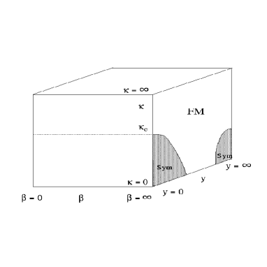
Figure 1: Phase diagram for XQCD.

When we couple the two models ($y_{0}\neq 0$), it is important to determine if the disorder of the $\Sigma$ sector can defeat the chiral breaking mechanism of the standard QCD action. There are no numerical results available in the region where $(\beta,\kappa,y_{0})$ are all finite. However an expansion in powers of $y_{0}$ can be easily performed, since this is the only coupling between the QCD and the $\Sigma$ sectors: $S_{XQCD}=S_{QCD}+S_{\Sigma}+y_{0}\sum_{x}{\bar{\psi}}_{x}\widetilde{\Sigma}_{x}\psi_{x}$.

To first nontrivial order in $y_{0}$, the order parameters $<\sigma>$ and $<{\bar{\psi}}\psi>$ for chiral symmetry breaking are

$$\langle\sigma\rangle = \langle\sigma\rangle_{\Sigma}-y_{0}\;\chi_{\sigma}\;\langle{\bar{\psi}}\psi\rangle_{QCD}+O(y_{0}^{2})~{},$$ (14)

$$\langle{\bar{\psi}}\psi\rangle = \langle{\bar{\psi}}\psi\rangle_{QCD}-y_{0}\langle\sigma\rangle_{\Sigma}\;\chi_{{\bar{\psi}}\psi}+O(y_{0}^{2}).$$ (15)

The VEV’s are ensemble averages in the QCD and $\Sigma$ sectors respectively,

$$\langle O\rangle_{QCD} = (1/Z_{QCD})\;\int[dUd{\bar{\psi}}d\psi]\;O\;e^{-S_{QCD}}$$

$$\langle O\rangle_{\Sigma} = (1/Z_{\Sigma})\;\int[d\Sigma]\;O\;e^{-S_{\Sigma}},$$

and $\chi_{{\bar{\psi}}\psi}$ and $\chi_{\sigma}$ are the corresponding susceptibilities.

Since we know that the QCD chiral symmetry is always broken ($\langle{\bar{\psi}}\psi\rangle_{QCD}\neq 0~{}$) for $0<\beta<\infty~{}$, it is clear from Eqs. (14) and (15) that XQCD must be in the broken phase $<\sigma>\neq 0,<{\bar{\psi}}\psi>\neq 0$ at any $\beta$ and $\kappa$ values in the small $y_{0}$ region. Intuitively, this result is easy to understand. A paramagnetic material will have nonzero magnetization in an external magnetic field. For XQCD, the QCD sector acts as an external symmetry breaking source to the scalar sector. Consequently, we are always guaranteed to be in the correct chiral phase for continuum QCD. To reach the continuum limit, we must approach the critical surface at $g^{2}_{0}=0$ without simultaneously tuning to the second order line at $\kappa_{cr}(y_{0})$. This additional “fine tuning” would introduce an unwanted finite mass scale for the Higgs field.

We have also explored the boundaries of the phase volume at the strong gauge coupling plane $\beta=0$ and at the strongly disordered chiral plane $\kappa=0$ to check that there is no sign of chiral symmetry restoration. We have carried out a perturbative study for the weak coupling limit of XQCD near $\kappa_{cr}$. As a result, we are confident that the only critical surfaces lie in the weak coupling plane at $\beta^{-1}\sim g^{2}_{0}=0$ as depicted in Fig. 1.

2.2 Toy Model Results

XQCD resembles earlier chiral quark models, such as the Georgi-Manohar (GM) model, in which both quarks and explicit pions have been introduced. However, unlike these models, XQCD is not meant to be a weak coupling effective theory. We do not assume new mass scales as implied by the condition, $\Lambda_{\chi SB}<<\Lambda_{QCD}$, introduced in the GM model. In XQCD, all “spurious” degrees of freedom must have masses at the cut-off scale. To understand how these properties might come about in a non-perturbative context, in a recent paper [5], we have investigated several toy models in the large N limit.

A natural toy model for XQCD is the Extended Nambu-Jona-Lasino model (XNJL), which couples the sigma model to a NJL model via a chirally invariant Yukawa term, $y_{0}{\bar{\psi}}(\sigma+i\gamma_{5}\vec{\tau}\cdot\vec{\pi})\psi$. Similar to our expectation for XQCD, the physical sigma resonance and pion in this extended model occur as a linear combination of elementary and composite operators: $(\sigma,\vec{\pi})$ and $({\bar{\psi}}\psi,{\bar{\psi}}i\gamma_{5}\vec{\tau}\psi)$, respectively.

We have demonstrated that the pseudoscalar mass spectrum is,

$$m_{\pi}^{2}=0\;\;;\;\;m_{\pi^{\prime}}^{2}=\Lambda^{2}\frac{y_{0}}{g_{0}^{2}}(\frac{<{\bar{\psi}}\psi>}{<\sigma>}+\frac{<\sigma>}{<{\bar{\psi}}\psi>}).$$

(Here, $g_{0}^{2}$ is the four-fermion coupling of the NJL model.) There is only one massless pion and the extra pion, $\pi^{\prime}$, resides at the cut-off scale. Similar results hold for the scalars. One mass, $m_{\sigma}$, which is proportional to the VEV, remains in the physical spectrum, while the other mass, $m_{\sigma^{\prime}}\sim m_{\pi^{\prime}}$, goes to infinity with the cut-off. Finally, we have verified that as the Yukawa coupling, $y_{0}$, is tuned to zero the spurious states remain at the cut-off. Just as we conjecture for XQCD, there is a smooth decoupling limit, where only the physical pion remains in the spectrum. In the limit of infinite cut-off XNJL and NJL models (at least at large N) are identical.

2.3 Constituent Mass Extrapolation.

We have started to do numerical simulations of XQCD with naive fermions using the $\phi$ algorithm [6], weighting the Trace-Log term appropriately for $n_{f}=2$. The simulations were performed on a 32-node CM5 using the CDPEAC routines of the BU-MIT collaboration code. For this preliminary investigation, the lattice size was $8^{4}$ at $\beta=5.6$ and $\kappa=0.3$. For QCD, we varied the fermion mass $m_{0}$ from $0.005$ to $0.1$, while for XQCD, we kept $m_{0}=0.0$ and varied $y_{0}$ from $0.01$ to $1.0$. All runs started from a cold Higgs field and a quenched gauge configuration at $\beta=5.8$. After performing $100$ trajectories each with 30 MD steps, we measured the number of iterations for the conjugate gradient (CG) algorithm to converge to a residue of $10^{-11}$. The results are plotted in Fig. 2.

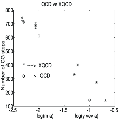
Figure 2: Comparison of the convergence rate for the conjugate gradient algorithm in QCD versus XQCD.

One concludes that we can simulate naive fermions exactly at the chiral point, $m_{0}=0$, without any convergence problem. Furthermore the convergence rate of CG for XQCD depends on the effective constituent mass $y_{0}<\sigma>$ of the fermions and it exhibits the same convergence rate as QCD compared at $m_{0}\simeq y_{0}<\sigma>$. Larger lattices with a variety of values for $(\beta,\kappa,y_{0})$ are under investigation to better estimate the relative efficiency between XQCD and QCD simulations.

The difficulty encountered with the standard QCD actions is the necessity to extrapolate from large bare quarks masses for u and d quarks ($\sim 50-200$ MeV) to the physical masses ( $\sim 5-10$ MeV). In XQCD, we may consider an alternative extrapolation in the constituent quark mass by taking the limit $y_{0}\to 0$. Obviously in this limit, XQCD becomes the standard lattice theory. In fact this approach is not so silly, if the limit is smooth and none of the spurious state are re-introduced into the low mass spectrum as $y_{0}\to 0$.

On the other hand, it should not be necessary to extrapolate to $y_{0}=0$. If we are in the same universality class, the fact that we regain continuum QCD as the lattice spacing goes to zero means that $y_{0}$ is an irrelevant parameter and the physical spectrum should be only weakly dependent on the value of $y_{0}$ over a range of small values of $y_{0}$. We are investigating numerically this range, but on intuitive grounds any value of $y_{0}$ which contributes a relatively small part of the 300MeV constituent mass should be safe.

3 DOUBLER PROBLEM

At first, it appears that a Wilson-Yukawa second order derivative term would be the ideal choice for removing doublers, because it preserves chiral invariance. At $g_{0}=0$, this leads to the Smit-Swift model which was studied extensively in the last few years. There it was found that a Wilson-Yukawa term either can not lift the doublers or removes all fermions from the spectrum [7].

However, there is one difference which appeared at first to allow a new solution. In our application, the VEV associated with the Higgs field can be taken to the cut-off. We have studied this scenario in the context of the XNJL toy model and found again that the spectrum looks fine, with one light pseudoscalar meson and both the doublers and the spurious scalar states at the cut-off. But there continues to be a fatal disease that looks to be very general. Namely in spite of the separation in mass scales, the value of $F_{\pi}$ for the Goldstone mode remains at the cut-off. Consequently we are not sanguine about this approach.

We are left with the options to use either the original Wilson term (5) or staggered fermions. The obvious problem with both choices is their explicit breaking of chiral U(2) symmetry. Both options require counter terms to restore (in the continuum limit) full chiral symmetry.

Before considering Wilson fermions in more detail, we remark that staggered fermions introduce very similar issues. One can couple the $\Sigma$ fields symmetrically to pairs of staggered flavors so that by the usual trick of taking the square root of the fermionic determinant, one is left with an SU(2) flavor form of XQCD. One nice feature of staggered fermions is that the U(1) center of the chiral SU(2) group is preserved so that vector Ward-Takahashi identities (WTI’s) alone can be used to restore the entire $SU(2)\times SU(2)$ current algebra. Nonetheless, we feel that the price one pays for the flavor symmetry breaking is still high and we prefer to use Wilson fermions.

4 COUNTER TERMS

Since the Wilson term breaks chiral invariance, the Ward-Takahashi identities (WTI’s) associated with chiral symmetry are no longer satisfied. One of these chiral Ward identities is the vanishing of the pion two point function at zero external momentum $G_{\pi\pi}^{-1}(0)=0$. For the standard Wilson formulation, it can be shown that to restore chiral symmetry in the continuum limit this is the only condition that must be met. Thus the non-perturbative mass counter term is introduced by tuning the bare quark mass $m_{0}=C_{0}\;a^{-1}+m_{q}$, where $m_{0}=C_{0}\;a^{-1}$ for a zero mass pion. (This is usually expressed in terms of the Wilson hopping parameter, $K=K_{crit}+O(a)$.)

4.1 Axial Vector Current

To restore chiral symmetry to XQCD, we must look at additional WTI’s. The full set of WTI’s is found by local chiral rotation for the integration variables in the path integral. For example, SU(2) chiral invariance leads to

$$<O\;\Delta_{\mu}A^{a}_{\mu}(x)>=<O\;{\bar{\psi}}\gamma_{5}\tau_{a}(m_{0}+\chi_{A})\psi>$$ (16)

where

$$A^{a}_{\mu}(x) = {\textstyle{1\over 2}}{\bar{\psi}}_{x}\tau_{a}\gamma_{\mu}\gamma_{5}U_{\mu}(x)\psi_{x+\mu}$$ (17)

$$+ {\textstyle{1\over 2}}\kappa Tr[\{\tau_{a},\Sigma^{\dagger}_{x}\}\Sigma_{x+\mu}]-h.c.$$

For simplicity we have taken $O$ to be chiral invariant. The $\chi_{A}$ term on the right comes from the variation of the Wilson term. To impose current conservation, we must introduce counter terms to cancel the singular and constant contributions of $\chi_{A}$ in the limit of zero lattice spacing.

As one may easily verify in lowest order perturbation theory, the set of local counter terms required to restore chiral symmetry is:

$$V_{CT} = \sum^{4}_{n=1}C_{n}Tr[(\Sigma)^{n}]+C_{5}Tr[(\Sigma_{x+\mu}-\Sigma_{x})^{2}]$$ (18)

$$+ h.c.+A\;{\bar{\psi}}\psi+B\;\bar{\psi}\widetilde{\Sigma}^{\dagger}\psi.$$

There are additional counter terms for the wave functions and the axial current, but these play a somewhat different role since they do not have to be introduced into the bare action prior to the simulations. They are only needed at the analysis stage.

4.2 Non-Perturbative Counter Terms

To fix the symmetry restoring counter terms, it is sufficient to consider two matrix elements ( the vacuum and the single quark matrix elements) of the WTI (16) with the $\Sigma_{x}$ field treated as an external source. Since the singular contributions only occur for orders up to $y^{4}_{0}$, it is convenient to expand for small $y_{0}$. By expanding in $y_{0}$, the path integral factorizes between the QCD and the $\Sigma$ sectors (see Section 2.1 ).

For example for the vacuum matrix element, one just computes term by term (up to $y^{4}_{0}$) the vacuum expectation values of

$$Tr[\gamma_{5}\tau_{a}\chi_{A}\frac{1}{M+{\textstyle{1\over 2}}y_{0}(\Sigma+\Sigma^{\dagger})+{\textstyle{1\over 2}}y_{0}\gamma_{5}(\Sigma-\Sigma^{\dagger})}]$$

in QCD at a fixed renormalized quark mass, $m_{q}=\mu$, computing the necessary traces by using the standard method of averaging over Gaussian pseudo fermionic sources. Each coefficient, $C_{n}(ay_{0},g_{0},a\mu,a)$, is then expressed as a low order polynomial in $y_{0}$, so that once it has been determined, XQCD is defined for a range of values of $y_{0}$ without re-computing the counter terms.

Table 1: One loop fermionic integrals.

$I_{n,m}$	m = 1	m = 2	m = 3	m = 4
n= 1	0.2347	0.8486	3.5421	16.318
n= 2	0.0259	0.0597	0.1925	0.7366
n= 3	(log-div)	0.0086	0.0165	0.0470
n= 4	(lin-div)	(log-div)	0.0031	0.0050

We are in the process of computing the counter terms non-perturbatively and comparing them with zeroth and first order expansions in $g^{2}_{0}$. To zeroth order, the single fermion loop contributes to $C_{n},n=1,..,5$:

$$C_{1} = \frac{2}{a^{3}}y_{0}\;I_{1,1}+\frac{2}{a}y^{3}_{0}\;I_{3,3}+O(g^{2}_{0}),$$

$$C_{2} = -\frac{1}{a^{2}}y^{2}_{0}\;I_{2,2}+2y^{4}_{0}\;(I_{3,2}-I_{4,4})+O(g^{2}_{0}),$$

$$C_{3} = \frac{2}{3a}y^{3}_{0}\;I_{3,3}+O(g^{2}_{0}),$$

$$C_{4} = -\frac{1}{2}y^{4}_{0}\;I_{4,4}+O(g^{2}_{0})$$

$$C_{5} = y^{2}_{0}\;I_{Z}+O(g^{2}_{0})$$

The single loop integrals are,

$$I_{n,m}=\int_{-\pi}^{\pi}\frac{d^{4}p}{(2\pi)^{4}}\frac{[rw(p)+a\mu]^{m}}{[g(p)]^{n}},$$ (19)

with $g(p)=\sum_{\mu}sin^{2}(p_{\mu})+(rw(p)+a\mu)^{2}$ and $w(p)=\sum_{\mu}(1-cos(p_{\mu}))$. The values at $\mu=0$ and $r=1$ are given in Table 1. Since the Wilson term vanishes at low momentum, no IR divergences occur in the chiral breaking terms to this order. The expression for the wave function renormalization integral, $I_{Z}$, is a little more complex but it has the finite value $I_{Z}=0.05473$. The first contributions to $A$ and $B$ are $O(g^{2}_{0})$.

For U(2) extended QCD, we also need to impose the WTI for the U(1) axial current. Due to the anomaly, this case is a little more intricate so we postpone it to a future publication.

5 CONCLUSIONS

The chiral extension of QCD, provides an improved action in which one is able to simulate near to or even at the chiral limit. Thus one can study the chiral vacuum at the physical mass of the pion. To avoid doublers, in the Wilson scheme, counter terms must be introduced, but they can be computed numerically in standard QCD at the decoupling point $y_{0}=0$. By studying the dependence of XQCD on the Yukawa coupling one can test its insensitivity to $y_{0}$, an important signal of universality. Also extrapolations in the constituent mass of the quark, $y_{0}$, afford an alternative to the current practice of extrapolating in the bare quark mass, $m_{0}$. We believe that being able to invert the XQCD quark propagator in the chiral limit is an important advantage of the chiral extension. Simulations are underway to determine if this is true.

References

- [1] G. Heatlie, C. T. Sachrajda, G. Martinelli, C. Pittori and G. C. Rossi, Nucl. Phys. B352, (1991) 266.
- [2] P. Hasenfratz, Nucl. Phys. B (Proc. Suppl.) 34, (1994) 3.
- [3] R. C. Brower, unpublished CERN (1992).
- [4] W. Bock, A. K. De, K. Jansen, J. Jersák, T. Neuhaus and J. Smit, Nucl. Phys. B344 (1990) 207.
- [5] R. C. Brower, Y. Shen and C-I Tan, “Chirally Extended Quantum Chromodynamics”, to be published in Phys. Rev. D (1994).
- [6] S. Gottlieb, W. Liu, D. Toussaint, R.L. Renken and R.L. Sugar, Phys. Rev. D 35 (1987) 2531.
- [7] For a recent review, see, D. N. Petcher, Nucl. Phys. B (Proc. Suppl.) 30 (1993) 50.