Latest Results from Heavy Quark Simulations

Abstract

I review the status of ${b\bar{b}}$ and ${c\bar{c}}$ calculations, numerical and analytic. I discuss the extraction of $\alpha_{s}$ and quark masses from spectrum calculations. I compare the NRQCD and Improved Heavy Wilson formulations of heavy quarks, and discuss recent calculations using a Heavy Staggered formulation.

1 Introduction

I have taken my charge in this review to be two-fold: to review this year’s results from heavy-heavy meson calculations and to compare the two main formalisms for treating heavy quarks, NRQCD[1] and the mass dependent improvement program of the Fermilab group[2] (which I call Improved Heavy Wilson(IHW) fermions). I will try to minimize my overlap with previous reviews[3, 4, 5]. The messages that I hope people take from the theory part of this talk are that IHW fermions are (improved) Wilson fermions (with an on-shell renormalization conditions), that NRQCD and IHW differ only by negligible irrelevant operators at large $am$, and that NRQCD actions have an extra symmetry (the heavy quark symmetry) which makes them much less messy to deal with but causes them to blow up at small $am$.

From the new results, my message is that we probably understand what we’re doing in onium systems; discretization errors, quenching effects, spin splittings and perturbation theory all seem to behave as expected. If this is true, then we are probably within one to three years of being able present an extensively cross-checked determination of ${\alpha_{\overline{\rm MS}}^{(5)}(M_{Z})}$, with uncertainty at the 1-2% level and all ingredients calculated in several different ways, to the rest of the particle physics community. Another message is that tadpole-improved coefficients[6] are necessary for perturbative improvement to work well. Finally, there is a discrepancy between typical lattice spacings determined from ${b\bar{b}}$ physics and those from light spectroscopy (both quenched and dynamical); we should be aware of this as a potential source of systematic error in light hadron calculations.

The reader should assume that any result reviewed here is preliminary, unless it appears elsewhere.

2 IHW and NRQCD: Compare, Contrast

2.1 A Toy Model

The most important feature of heavy quark ($am$$\stackrel{{\scriptstyle\textstyle{>}}}{{\sim}}$$1$) calculations on the lattice is that, for a lattice O(4) invariant action, boost invariance of on-shell correlation functions is strongly broken, even for soft boosts of particles with (spatial) momentum much smaller than the cutoff. This is because all components of the on-shell four-momentum cannot be made small simultaneously; the energy will always be of order the cutoff or higher. To restore low-momentum boost invariance without taking the cutoff much larger than the mass, (lattice) boost invariance must be broken in the bare action; lattice O(3) is the appropriate symmetry group for heavy quark bare actions. NRQCD implements the breaking O(4)$\rightarrow$O(3) directly; NRQCD is a non-relativistic effective action. In the IHW formalism the breaking is more subtle; the IHW formalism can be thought of as just the normal improvement program for Wilson fermions, except the renormalization conditions are imposed with the heavy quark on-shell[7]. The Lorentz breaking arises because the four-momentum of a heavy quark is very anisotropic; a ‘preferred frame’ is chosen which is just the rest frame of the heavy quark.

To illustrate this, consider the dispersion relation of an on-shell (free) naive fermion;

$$(am)^{2}+\sum_{\mu}\sin^{2}(ap_{\mu})=0.$$ (1)

If $am\ll 1$, all of the components of the dimensionless momentum can be chosen small, so that $\sin$ can be replaced with its expansion;

$$(am)^{2}+(ap)^{2}-{{1}\over{3}}\sum_{\mu}(ap_{\mu})^{4}+\dots=0,$$ (2)

where $(ap)^{2}$=$\sum_{\mu}(ap_{\mu})^{2}$. The first two terms in (2) represent the continuum dispersion relation, while the third and later terms are cutoff effects. Since these are much less than one, (2) is approximately Lorentz invariant at low momenta.

When $am$ is large, however, this fails. At least one component (the energy) of the 4-momentum in (1) must be large, so as to cancel the mass term, and the $\sin$ of this component cannot be expanded. This leads to the dispersion relation

$$(am)^{2}+\sin^{2}(ap_{0})+(a{\bf p})^{2}-{{1}\over{3}}\sum_{i}(a{\bf p}_{i})^{4}+\dots=0,$$ (3)

where ${\bf p}$ is the spatial momentum. Even at low momenta, (3) is not Lorentz invariant, and so the bare action that leads to it cannot be used directly to calculate S-matrix amplitudes. Discretization errors in the temporal and spatial directions are different; to obtain the correct behavior near the mass-shell the temporal and spatial terms in the action must be adjusted separately. This results in an action which only has lattice O(3) symmetry, but which has O(4) invariant correlation functions at low momentum.

The dispersion relation (3) has behavior very similar that of IHW fermions[7, 4]; the static mass, $M_{1}$, depends logarithmically on $am$ when $am\gg 1$, while the kinetic mass, $M_{2}$, goes linearly with $am$. A Lorentz invariant theory has $M_{1}$=$M_{2}$=$M_{3}$=$\dots$, where $M_{3}$ is the mass appearing in the ${\bf p}^{4}$ term in the relativistic low momentum dispersion relation. $M_{1}$=$M_{2}$ can be recovered by rescaling the spatial derivatives relative to the temporal derivatives; this is equivalent to the ‘asymmetric $\kappa$’ prescription in [7]. $M_{3}$ must be adjusted by adding a ${\bf p}^{4}$ improvement term to the action; note that this is a lattice O(3), rather than lattice O(4), invariant operator. For Wilson fermions, the clover term, $\bar{\psi}\sigma_{\mu\nu}F^{\mu\nu}\psi$, is the lowest order improvement operator needed in the action[8]. When $am\gg 1$, the asymmetric physical renormalization point requires that $\sigma\cdot F$ be broken up into a sum of electric and magnetic O(3) invariant representations, with separately tuned coefficients for the electric and magnetic terms. I will call this the ”asymmetric clover” level of improvement for the IHW formulation.

The Fermilab group has pointed out that only a modified Lorentz invariance is needed when studying processes involving valence heavy quarks; rather than using an asymmetric $\kappa$ to tune $M_{1}$=$M_{2}$, one can shift the zero of energy in the continuum theory by $M_{2}-M_{1}$ for each quark without changing the physics. If this is true, then $\kappa$ can be kept symmetric as long as $M_{1}$ is ignored. This is typically done both in IHW and NRQCD. Asymmetric improvement terms are still needed at higher orders; for example an asymmetric clover coefficient is needed to get both spin-spin and spin-orbit interactions right.

2.2 Similarities and Differences

IHW and NRQCD are very similar formalisms for simulating heavy quarks. Both break lattice O(4) invariance to lattice O(3) in the bare action to recover boost invariant low momentum correlation functions. Both rely heavily on an improved action program to eliminate discretization errors, and the systematic errors in both can be expanded in ${\Lambda_{QCD}}/M_{Q}$ (where ${\Lambda_{QCD}}\sim 500{\rm MeV}$). Although the IHW is formulated in terms of Dirac spinors, it can be thought of in the Foldy-Wouthuysen-Tani(FWT) transformed basis of NRQCD.

There is an intrinsic difference between the two formalisms, however. In the FWT basis, NRQCD throws away the coupling between large and small components of the 4-component spinors, resulting in a block diagonal action involving (2 sets of) 2-component Pauli spinors. This imposes an additional symmetry on the action (the heavy quark symmetry), and causes the NRQCD action to be non-renormalizable when $am\rightarrow 0$. The advantage of this procedure is that $m$ can be removed as a scale before discretization. The IHW action does not eliminate the couplings between large and small components and so is renormalizable (going over into an improved Wilson action as $am\rightarrow 0$), at a cost of having to treat discretization errors to all orders in $am$.

To illustrate the difference, start with the free continuum Dirac action (note that neither NRQCD nor IHW is actually derived as below, but the basic principles are the same);

$$S_{Dirac}=\bar{\psi}\left(\begin{array}[]{cc}\partial_{t}+m&i{\mbox{\boldmath$\sigma$}}\cdot{\bf p}\\ i{\mbox{\boldmath$\sigma$}}\cdot{\bf p}&-\partial_{t}+m\end{array}\right)\psi.$$ (4)

A continuum FWT transformation can now be performed to some order in $v^{2}$=$({\bf p}/m)^{2}$, resulting in (for the lowest order transformation)

$$\bar{\psi}\left(\begin{array}[]{c}\partial_{t}+m+{{{\bf p}^{2}}\over{2m}}+\dots\quad\dots\\ \dots\quad-\partial_{t}+m+{{{\bf p}^{2}}\over{2m}}+\dots\end{array}\right)\psi,$$ (5)

where $\dots$ represents terms which lead to higher order corrections to the dispersion relation, such as ${\bf p}^{4}/m^{3}$. If we discretize (5) directly, we obtain

$$\bar{\psi}\left(\begin{array}[]{ll}a^{-1}\sinh(aE)+m+{{{\bf p}^{2}}\over{2m}}+\dots\quad\dots\\ \dots\quad-a^{-1}\sinh(aE)+m+{{{\bf p}^{2}}\over{2m}}+\dots\end{array}\right)\psi,$$ (6)

This is the IHW approach; as m gets large, $\sinh(aE)$ and hence $aE$ must also become large, leading to large discretization errors. In the NRQCD approach, the higher order terms ($\dots$) in (5) are set explicitly to zero. This makes (5) block-diagonal; the transformation $\bar{\psi}\rightarrow\bar{\psi}e^{m\gamma_{0}t}$, $\psi\rightarrow e^{-m\gamma_{0}t}\psi$ can now be performed on (5), resulting in an action

$$S_{NR}=\bar{\psi}\left(\begin{array}[]{ll}\partial_{t}+{{{\bf p}^{2}}\over{2m}}\quad 0\\ 0\quad-\partial_{t}+{{{\bf p}^{2}}\over{2m}}\end{array}\right)\psi.$$ (7)

This is the NRQCD approach; ${{a{\bf p}^{2}}\over{2m}}$ is O($mv^{2}$), so there are no problems discretizing (7). When $am\rightarrow 0$, the symmetry imposed by the zero entries in (7) is no longer valid; the theory cannot be renormalized. This method for removing the zero of energy doesn’t work for IHW; $\gamma_{0}$ doesn’t commute with the off-diagonal components of (5).

2.3 Pros and Cons

In IHW, discretization errors must be treated to all orders in $am$. In NRQCD, $m$ has been removed as a dynamical energy scale, and discretization errors can be expanded in $a{\bf p}$. This means that:

• In IHW, the tree-level coefficients of terms in the action are complicated, non-intuitive functions of $am$. In NRQCD, these coefficients are simple functions, for which non-relativistic intuition can be easily applied.

• NRQCD is a non-renormalizable theory; the coefficients in the NRQCD action blow up when $am$$\stackrel{{\scriptstyle\textstyle{<}}}{{\sim}}$$.6$ (see Fig. 1). An IHW action is renormalizable; as $am\rightarrow 0$ it goes smoothly over to a perturbatively improved Wilson action.

• Because NRQCD blows up at small $am$, charm can only be simulated at $\beta$$\stackrel{{\scriptstyle\textstyle{<}}}{{\sim}}$$5.85$. IHW simulations can be performed at any $\beta$; brute force can be used to reduce discretization errors and there is a much larger range of $\beta$ for which charm and bottom quarks can be simultaneously studied.

• Because of the complicated coefficients, the IHW action is harder to derive than NRQCD. To date, only the terms which contribute at leading order in $v^{2}$ to the spin-averaged and spin dependent spectra have been published for the tree-level IHW action. The relativistic corrections to these terms have been published, also at tree level, for NRQCD.

• IHW fermions cost more CPU time than NRQCD; IHW propagators solve an elliptic partial differential equation(PDE), while NRQCD solves a parabolic PDE. I suspect the IHW inverter can be accelerated. When $am$ is large, the IHW PDE is close to parabolic; there should be a way to use this.

2.4 Levels of Improvement

I find it easiest to use the NRQCD action derived in [1] to catalogue improvement terms in the NRQCD or IHW actions and to understand their effects. The O($mv^{4}$) NRQCD action is given by

$$S = \bar{\psi}(\Delta_{t}+H)\psi.$$

$$H = -{\Delta^{(2)}\over 2{M_{0}}}$$ (8)

$$-C_{1}\frac{(\Delta^{(2)})^{2}}{8({M_{0}})^{3}}+C_{2}\frac{ig\left({\bf{\bf\Delta}}\cdot{\bf E}-{\bf E}\cdot{\bf{\bf\Delta}}\right)}{8({M_{0}})^{2}}$$

$$-C_{3}\frac{g{\mbox{\boldmath$\sigma$}}\cdot({\bf{\bf\Delta}}\times{\bf E}-{\bf E}\times{\bf{\bf\Delta}})}{8({M_{0}})^{2}}-C_{4}\frac{g{\mbox{\boldmath$\sigma$}}\cdot{\bf B}}{2{M_{0}}}\,$$

$$+C_{5}\frac{a^{2}{\Delta^{(4)}}}{24{M_{0}}}-C_{6}\frac{a(\Delta^{(2)})^{2}}{16n({M_{0}})^{2}},$$

where $\Delta^{(2)}$ is the discrete laplacian, and ${\Delta^{(4)}}$=$\sum_{i}\Delta_{i}^{4}$. For HH mesons, the $C_{i}$ terms all contribute O($mv^{4}$) to the energy; the kinetic energy term is, of course, O($mv^{2}$). Further improvement operators are suppressed by more powers of $v^{2}\sim{\Lambda_{QCD}}/M$, which is about $.1$ for ${b\bar{b}}$ and $.3$ for ${c\bar{c}}$. The counting for improvement operators is different in HL mesons; see [1] for details. All operators are tadpole-improved; $C_{i}$=$1$ at tree-level.

The terms in (8) are easily identified from low energy electrodynamics; $C_{1}$ multiplies the leading relativistic correction to the dispersion relation, $C_{2}$ the Darwin term, $C_{3}$ the spin-orbit coupling (causing fine-structure), and the $C_{4}$ term gives rise to the spin-spin interaction (causing hyperfine splittings). The $C_{5}$ and $C_{6}$ terms correct the leading discretization errors in the spatial and temporal directions, respectively.

As more accuracy and physical information is required from a heavy quark calculation, more improvement terms can be turned on in the action. For every NRQCD action, there is a corresponding IHW action[2] in which similar improvement terms have been turned on. At large $am$, the effects of improvement terms which have not yet been turned on should be the same size in IHW and NRQCD. At small $am$, however, the IHW action recovers lattice O(4) invariance, so the effects of lattice O(4) breaking improvements are small. In NRQCD language, the Wilson action gets the term corresponding to $C_{1}$ right at small $am$, without needing improvement. In this regime, it is much harder to estimate the IHW systematic errors and compare to O($mv^{4}$) NRQCD, for example. El-Khadra has used potential models to estimate these errors in the Fermilab group’s calculations[9], but it is also important to obtain simulation results from the IHW action equivalent to (8), so that the two methods can be directly compared.

The simplest action to calculate with is just O($mv^{2}$) NRQCD, in which all the $C_{i}$ terms in (8) are turned off. This is a spin-symmetric action; spin-averaged splittings will have errors at the $v^{2}$ level, but spin dependent splittings will be zero. The equivalent IHW action is just the normal Wilson action; spin splittings are non-zero but much too small. Note that the $C_{1}$ and $C_{2}$ terms contribute to the kinetic mass at the $v^{2}$ level; if more precision is needed for $M_{2}$ then these improvements (and probably $C_{5}$ and $C_{6}$) should be turned on.

To study spin splittings, the $C_{3}$ and $C_{4}$ improvements must be turned on. In IHW, this is equivalent to turning on the clover term; the magnetic part corresponds to the $C_{4}$ term, while the electric part is the sum of $C_{2}$ and $C_{3}$ improvements. The Sheikholeslami-Wohlert action[8] has the correct $C_{4}$ improvement, but $C_{3}$ and $C_{2}$ are somewhat wrong. This is fixed by going to the asymmetric clover action; at tree-level, the $C_{2}$, $C_{3}$, and $C_{4}$ terms are all correctly included.

The most complicated action in use is the $mv^{4}$ NRQCD action in (8). Errors in spin averaged splittings and kinetic masses should be at the $v^{4}$ level, while spin splittings still have $v^{2}$ errors. The corresponding IHW action is not published; it is important that IHW calculations be done at this order to compare with NRQCD results.

If one wants to reduce errors in the spin splittings to O($v^{4}$), then one must go to the level of improvement in [1]. This is the first level at which one-loop results are needed for the $C_{i}$. Since $\alpha_{s}$ should be about the same size as $v^{2}$, the $\alpha_{s}mv^{4}$ errors arising from the use of tree-level $C_{i}$ should be about the same size as $mv^{6}$ improvement terms. (Note that I have used this to simplify the discussion of errors above. $v^{4}$ errors really means $v^{4}$ and $\alpha_{s}v^{2}$ errors; both should be the same size.) Until the one-loop corrections to $C_{3}$ and $C_{4}$ (or their IHW equivalents) are known, this level of improvement cannot be fully implemented.

The results presented this year have different levels of improvement for different groups. The $mv^{2}$ NRQCD action was used by the UK(NR)QCD group[10], and by Bodwin, Kim and Sinclair[11], who have performed a very nice calculation of matrix elements involved in ${b\bar{b}}$ decay. The KT group[12, 13] and Wingate et al.[14] (referred to as KT and CDHW below) both use a Wilson action, which should have similar errors. The Fermilab group[9] uses the SW action; the NRQCD collaboration [15, 16, 17] uses the $mv^{4}$ NRQCD action. Both use tadpole improvement, which is essential.

3 Perturbation Theory

Perturbative calculations are an essential ingredient in both the NRQCD and IHW formalisms. To date, NRQCD and IHW simulations have been done using only tree-level coefficients for the improvement terms in the action. The next level of relativistic corrections, O($mv^{6}$), however, are about the same size as the one-loop corrections to the current action, O($\alpha_{s}mv^{4}$), so loop calculations are needed to improve the actions beyond O($mv^{4}$). Besides the action, perturbation theory is needed for non-spectroscopic results. For example, a calculation of the pole or ${\overline{\rm MS}}$ quark masses requires a perturbative calculation of the quark dispersion relation, while wave function and current renormalizations will be needed for quantities such as $f_{B}$ or the leptonic width of onium.

The Fermilab group has an ongoing program to perform perturbative calculations for the IHW formalism[9, 18, 19, 20], while Morningstar has performed most of the recent perturbative calculations in NRQCD[21, 22]. Both calculate the dispersion relation of the heavy quark; matching to the low energy continuum dispersion relation then fixes the $C_{1}$, $C_{5}$, and $C_{6}$ improvements, as well as the corrections needed to determine the pole or ${\overline{\rm MS}}$ mass[17]. The main new results this year are the inclusion of the Lepage-Mackenzie $q^{*}$ in these perturbative calculations[22, 9, 19].

Figure 1: Calculation by Morningstar [22] of the 1-loop perturbative correction to the coefficients $C_{1}$, $C_{5}$, and $C_{6}$ in the NRQCD action as a function of aM. Note that Morningstar’s $c_{1}$ corresponds to a combination of $C_{1}$ and $C_{6}$, while $c_{2}$ is $C_{5}$ in (8).

The corrections to the action appear well behaved in both formalisms; Morningstar’s results for the one loop contribution to the $C$’s are shown in Fig. 1. The one-loop correction is roughly 10% for $am>.8$; this is a good indication that perturbation theory is working. Notice that the corrections begin to grow rapidly below $am<.6$; this is where NRQCD begins to “blow up.”

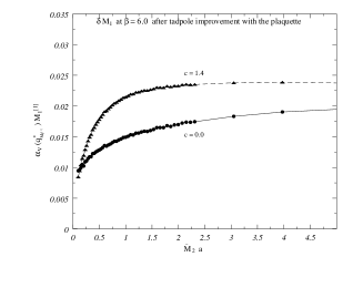
Figure 2: Perturbative correction to the static mass ($M_{1}$) for both Wilson ($c$=$0$) and SW ($c$=$1.4$) actions as a function of the kinetic mass ($M_{2}$)[23].

The Fermilab group has similar results for the perturbative correction to the static mass; their results for both SW and Wilson actions are shown in Fig. 2. Again, the result is very well-behaved. This calculation can be combined with simulation results to determine the quark’s pole mass[9].

4 Heavy Staggered Fermions

This year, the KT group has introduced a third heavy fermion formalism; Heavy Staggered (HS) fermions[24]. They have performed simulations at both quenched $\beta$=$6.0$ and at $n_{f}$=$2$ staggered, $\beta$=$5.7$, $am_{s}$=$.01$[25], with bare valence masses ranging from $am_{Q}$=$.2$ to $am_{Q}$=$.5$. They used static, rather than kinetic, masses to match with experiment, but at these values of the $am$ this is probably not a huge effect. As with most staggered fermion calculations, they had to deal with a daunting number of meson creation operators; they used 128 operators grouped into 36 irreducible representations!

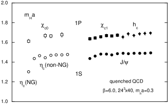
Figure 3: Heavy staggered ${c\bar{c}}$ spectrum. NG refers to flavor singlet pseudoscalar. Different points correspond to different irreducible lattice representations of the continuum state[24].

Results for the ${c\bar{c}}$ spectrum (averaged within irreducible representations) are shown in Fig. 3. As can be seen in the figure, the masses of the states are dependent on the particular operator used. Furthermore, this operator dependence seems to go like the square of the heavy mass[24]. The most pronounced of these splittings is between the flavor singlet and flavor non-singlet versions of the $\eta_{c}$; the KT group quotes separate results for the ‘NG’ and ‘non-NG’ pseudoscalars.

Figure 4: Finite volume dependence of HS ${c\bar{c}}$ states. Note the large shift in the $h_{c}$ state. [24]

A result that may be of concern to those using other formulations for ${c\bar{c}}$ is shown in Fig. 4, which compares HS results at quenched $\beta$=$6.0$ on $16^{3}$x$40$ and $24^{3}$x$40$ lattices. The change of about 3% in the mass of the $h_{c}$ results in a 20% change in the $1{\rm S}$-$1{\rm P}$ splitting. The smaller lattice is roughly the same physical size as most of those which have been used for ${c\bar{c}}$ simulations; an explicit check of volume dependence in ${c\bar{c}}$ spectroscopy should probably be done using the IHW or NRQCD formulation. This is much less likely to be a problem in ${b\bar{b}}$ spectroscopy; the ${b\bar{b}}$ mesons are much smaller than ${c\bar{c}}$.

The KT group has extracted a value of ${\alpha_{\overline{\rm MS}}^{(5)}(M_{Z})}$ from the ${c\bar{c}}$ $1{\rm P}$-$1{\rm S}$ splitting; they obtain $.111(4)(2)$ from their quenched results and an upper bound of $.119(3)(3)$ at $n_{f}$=$2$, where the first uncertainty is from the scale determination and $n_{f}$ correction and the second comes from flavor breaking. They have asked me to stress that, because of the strong finite volume dependence of the $h_{c}$ mass, the $n_{f}$=$2$ result should only be considered an upper bound.

5 Onium Spectroscopy

5.1 ${b\bar{b}}$

Three groups have calculated more than one splitting in the ${b\bar{b}}$ spectrum recently. This year, the Fermilab[26, 9] and NRQCD[27, 15] groups have increased their quenched statistics and the NRQCD group has results at $n_{f}=2$. The results for spin averaged splittings are shown in Fig. 5. The Fermilab group determines the lattice spacing from the $1{\rm P}$-$1{\rm S}$ splitting; the NRQCD collaboration uses both the $1{\rm P}$-$1{\rm S}$ and the $2{\rm S}$-$1{\rm S}$ splitting. The zero of energy in Fig. 5 is adjusted so that the $\Upsilon(1{\rm S})$ energy matches experiment; the bare mass of the $b$ quark is adjusted so that the kinetic mass, $M_{2}$, of this state agrees with its experimental value.

Figure 5: Spin averaged ${b\bar{b}}$ spectrum. A horizontal line indicates the experimental energy; experimental values for spin-singlet $P$ states are assumed to equal spin average of the corresponding triplet states. Results are shown at $\beta$=$5.6$ ($n_{f}$=$2$ NRQCD), 6.0 ($n_{f}$=$0$ NRQCD), 6.2 (UK(NR)QCD), and 6.1 (Fermilab).

The discretization and relativistic errors in Fig. 5 are expected to be about 5MeV for the NRQCD group, 50MeV for UK(NR)QCD[10], and somewhere between the two for Fermilab. This is because the NRQCD collaboration includes all O($mv^{4}$) terms in the action, while UK(NR)QCD only works at O($mv^{2}$). The clover action used by Fermilab has an incorrect coefficient for the ${\bf p}^{4}/(8m^{3})$ term in the action, which becomes correct as $am\rightarrow 0$; the error in this coefficient controls the size of O($mv^{4}$) errors in the Fermilab results.

The NRQCD collaboration has spectrum results at $n_{f}$=$2$. These use an ensemble obtained from the HEMCGC collaboration, with two flavors of staggered fermions at $am$=$.01$ and $\beta$=$5.6$[28]. The CDHW results, which I will discuss later, used this ensemble and a similar one (also from HEMCGC) at $am$=$.025$. The only other dynamical results available are from the KT group, who worked at $\beta$=$5.7$ rather than $5.6$[25]. Both the CDHW and KT groups have results only for the $1{\rm P}$-$1{\rm S}$ splitting.

The HEMCGC collaboration has performed a tremendous public service by making their ensembles publicly available; given the high cost of generating dynamical ensemble, it is important that as much analysis as possible be done on each one. Many other groups have been similarly generous in providing their quenched ensembles to the NRQCD collaboration.

The results show excellent agreement with experiment. The most important thing to focus on in Fig. 5 is the relative size of the $2{\rm S}$-$1{\rm S}$ and $1{\rm P}$-$1{\rm S}$ splittings; their ratio is plotted in Fig. 6 as a function of $n_{f}$. It appears that there is a discrepancy in this ratio at $n_{f}$=$0$, $(2{\rm S}$-$1{\rm S})/(1{\rm P}$-$1{\rm S})$=$1.41(5)$, when compared with the experimental value of 1.28, and that this discrepancy is removed when extrapolated to an $n_{f}$ value between $2$ and $4$. Fig. 6 also shows consistent, but noisier, results at $\beta$=$5.7$. This is an encouraging indication of scaling, but it should be noted that this splitting has been adjusted by a large ($\approx$$40{\rm MeV}$) perturbative correction which removes O($a^{2}$) errors in the gluonic propagator[15, 16]; The NRQCD collaboration results may also show a quenching effect for the $2{\rm P}$-$1{\rm P}$ splitting; this is not supported, however, by the UK(NR)QCD results.

Figure 6: Dependence on $n_{f}$ of the ratio of the $2S-1S$ to $1P-1S$ splittings in $b\overline{b}$. The filled circles give values at quenched $\beta$ = 6.0 and $\beta$=5.6, $n_{f}$=2. The open circle is quenched $\beta$ =5.7 for comparison. The horizontal dashed line gives the experimental value of 1.28 and solid line is an extrapolation to $n_{f}$ = 3, drawn to guide the eye. All results are from the NRQCD collaboration[15].

Fig. 6 exhibits exactly the behavior one expects from quenching errors; determining $a^{-1}$ from the $1{\rm P}$-$1{\rm S}$ splitting is roughly equivalent to matching the force in the quenched static potential at the Bohr radius to be the same as the force in full QCD, i.e. $\alpha_{n_{f}=0}(r_{0})$=$\alpha_{full}(r_{0})$ (this is the essence of the Fermilab prescription for correcting quenching errors in $\alpha_{s}$ determinations[29]). Since the quenched $\beta$-function runs faster than the full one, the potential $\alpha(r)/r$ will be weaker than it should be at short range. This in turn should shift quenched $S$ states up relative to the $P$ states. The charm quark is too heavy to affect the running of $\alpha$ at the Bohr radius of $\Upsilon$, so the spin-averaged spectrum should agree with experiment when extrapolated to $n_{f}$=$3$.

Figure 7: ${b\bar{b}}$ spin splittings. The expected (non-quenching) systematic error in the NRQCD calculation is shown; the Fermilab results should have similar errors. Symbols are the same as in Fig. 5.

The NRQCD and Fermilab groups have also calculated spin splittings in the ${b\bar{b}}$ system; the results are shown in Fig. 7. The (non-quenching) systematic errors are expected to be about $5{\rm MeV}$ for both groups, and are indicated in the figure.

The most important feature of Fig. 7 is that the overall size of the $\chi_{b}$ splittings agrees with experiment, within the expected errors. This is significant for two reasons. First, both the Fermilab and NRQCD actions are tadpole improved, which increases the strength of the spin interactions by a factor of $u_{0}^{-3}$; without tadpole improvement the $\chi_{b}$ splittings are reduced by 50%[30]. Second, spin splittings are quadratically sensitive to the lattice spacing. This is because they are roughly inversely proportional to the quark mass. Using an incorrectly low value of $a^{-1}$ to compare with experiment will result in tuning to too heavy a quark mass; this reduces the dimensionless spin splittings, which are then multiplied by an additional factor of (the incorrect) $a^{-1}$ to make them dimensionful. If the correct lattice spacing for $\Upsilon$ physics at $\beta$=$6.0$ were $2.0{\rm GeV}$ rather than the $2.4{\rm GeV}$ found by the NRQCD collaboration, the $\chi_{b}$ splittings in Fig. 7 would be roughly 30% smaller in magnitude, resulting in a 15-20MeV disagreement with experiment.

The quenched ratio $(\chi_{b2}-\chi_{b1})/(\chi_{b1}-\chi_{b0})$ appears too small compared to experiment; adding dynamical fermions pushes the ratio the wrong way. Although this is only a one to two $\sigma$ effect, the same behavior occurs with good statistical significance in the ${c\bar{c}}$ system. In both ${b\bar{b}}$ and ${c\bar{c}}$ the disagreement with experiment is within the expected systematic errors. It will be interesting to see if improving the NRQCD or IHW actions to eliminate O($v^{2}$) corrections to the spin-splittings will fix this discrepancy.

Unfortunately, the $\eta_{b}(1S)$ has not been observed experimentally; extrapolating the NRQCD results to $n_{f}$=$3$ (where $a^{-1}$ and $m_{0}$ have been adjusted) results in a hyperfine splitting of $44{\rm MeV}$[15]. Because the hyperfine splitting is a short-distance quantity, dynamical charm loops are likely to have an effect, but a simple perturbative estimate indicates that this is likely to be at most a few MeV. The result should be somewhere between $45$ and $50{\rm MeV}$, which agrees with what is expected from potential models.

5.2 ${c\bar{c}}$

Both the NRQCD[15, 31] and Fermilab [9, 26] groups have increased their statistics for quenched ${c\bar{c}}$ spectroscopy. I do not show the spin averaged spectrum, since the only independent level is the $2{\rm S}$, which is too noisy to resolve quenching effects. Instead, the spin-dependent spectrum is shown in Fig. 8, along with the expected (non-quenching) systematic errors (estimated to be roughly $35{\rm MeV}$), which are much larger than for ${b\bar{b}}$ since $v^{2}$ is three times as big. The interesting thing about Fig. 8 is that these systematic errors are dominant; the statistical errors are negligible. Within the (rather large) systematic uncertainty, Fig. 8 shows agreement between simulation and experiment. In addition, the trends seen in ${b\bar{b}}$ spin splittings (Fig. 7) are now quite clear; hyperfine and fine splittings are too small and the ($\chi_{c2}-\chi_{c1}$)/($\chi_{c1}-\chi_{c0}$) ratio is too big.

Figure 8: ${c\bar{c}}$ spin splittings. Symbols are same as Fig. 5. Levels are adjusted so that spin averaged energies agree with experiment.

The bad news from Fig. 7 is that ${c\bar{c}}$, for which there is more experimental data, is not as well controlled a system as ${b\bar{b}}$ is. This was to be expected; in addition to suffering from worse relativistic corrections, ${c\bar{c}}$ is a larger meson with softer internal glue, and so is more susceptible to finite volume effects and the particulars of the dynamical fermion content. For these reasons, I suspect that the ${b\bar{b}}$ system is probably more reliable for $\alpha_{s}$ determinations than ${c\bar{c}}$.

The good news is that ${c\bar{c}}$ is a wonderful laboratory for studying improved actions; the effects of (currently neglected) O($mv^{6}$) and O($\alpha_{s}mv^{4}$) terms in the NRQCD action are resolvable. A drop in the disagreement with experiment of the ${c\bar{c}}$ spin spectrum of a factor of 3 or so (i.e. $v^{2}$) upon inclusion of these terms (or similar ones in the IHW approach) would be a tremendous result showing the efficacy of improved actions.

A final comment: the validity of the IHW formalism at any value of $am$ is a definite advantage for charm physics. As presently formulated, NRQCD blows up for charm at roughly (quenched) $\beta$=$5.85$, but has a much more easily computed improved action. A IHW action, improved to the some order in $v^{2}$ and $\alpha_{s}$, will almost certainly have smaller systematic errors when run at a high $\beta$ than the similarly improved NRQCD action run at $\beta_{max}$=$5.85$ will have. On the other hand, the IHW run (say at $\beta$=$6.4$) will probably cost 100 times as much computer time at the same physical volume. Today, with IHW actions in use which are less highly improved than the NRQCD actions, the relative size of systematic errors is unclear. For ${b\bar{b}}$ physics, this advantage of IHW does not yet enter; even at $\beta$=$6.4$, $am$$\approx$$1$ and NRQCD can be used.

6 $M_{b}$

Last year, the NRQCD collaboration presented a preliminary result for the pole mass of the bottom quark[30]. The final results of this calculation can be found in [17], which also includes the effects of dynamical fermions and a determination of the ${\overline{\rm MS}}$ mass. This year the Fermilab group has presented a preliminary determination of the pole mass of the charm quark [9].

The basic idea is very simple; given a particular regularization scheme (i.e. ${\overline{\rm MS}}$, IHW, or NRQCD), the perturbative pole mass can be calculated in terms of the mass parameter of the theory.

$$M=Z_{m}^{S}\,\,m_{0}^{S}=(1+C^{S}\alpha_{s}(q^{*}))m_{0}^{S},$$ (9)

where $S$ labels the scheme, $C^{S}$ is calculated in perturbation theory, and $q^{*}$ is a scale chosen as in [6] or [32]. The ${\overline{\rm MS}}$ mass can be obtained by equating the pole mass in the ${\overline{\rm MS}}$ and lattice schemes;

$$M^{{\overline{\rm MS}}}(M)={Z_{m}^{NR}\over Z_{m}^{{\overline{\rm MS}}}}\,m_{0}^{NR}={Z_{m}^{IHW}\over Z_{m}^{{\overline{\rm MS}}}}\,m_{0}^{IHW}.$$ (10)

The bare mass of the lattice theory (IHW or NRQCD) is determined by requiring that the kinetic mass of the ground state match experiment; the result is substituted into (9) to obtain the pole mass or (10) to obtain the ${\overline{\rm MS}}$ mass.

The NRQCD collaboration obtains a pole mass for bottom of $M_{b}$=$5.0(2)$ and an ${\overline{\rm MS}}$ mass of $M_{b}^{{\overline{\rm MS}}}(M_{b})$=$4.0(1)$[17]; the Fermilab group has a preliminary result of $M_{c}$=$1.5(2)$[9].

A word of caution: the NRQCD collaboration result has changed since last year. This is because $q^{*}$ is actually much softer than the preliminary estimate used in[30]; $\alpha_{V}(q^{*})$$\approx$$.4$ for the bottom quark at $\beta$=$6.0$. This soft scale arises because tadpole improvement cancels out the contribution to $q^{*}$ of much of the hard glue. A soft $q^{*}$ also appears in the ${\overline{\rm MS}}$ scheme; applying the procedure of [32] to the two-loop ${\overline{\rm MS}}$ expression for the pole mass[33] gives $q^{*}$$\approx$$.22\,M_{b}$. Because of these soft $q^{*}$s, perturbative uncertainties dominate the NRQCD determination of $M_{b}$, and make an NRQCD determination of $M_{c}$ impossible. Soft $q^{*}$s are less of a problem in the ${\overline{\rm MS}}$ mass determination; the soft glue cancels in the ratio of $Z$s, leaving a $q^{*}$ closer to the cutoff. It is not clear what non-perturbative effects there might be in equating the (perturbative) pole masses of two different schemes, especially since infra-red glue seems to be playing such an important role. The Fermilab group has not found a similar soft $q^{*}$ in their IHW calculation.

7 $\alpha_{s}$

Last year, El-Khadra gave an excellent review of $\alpha_{s}$ determinations from onium spectroscopy[34], so I will not go into detail. At that meeting, there were quenched results from the NRQCD and Fermilab groups, as well as preliminary dynamical results from the KT group, using their $n_{f}$=$2$ staggered, $\beta$=$5.7$ ensemble. This year, the KT[12], CDHW[14] and NRQCD[16] groups have new dynamical results, using KT , HEMCGC, and HEMCGC ensembles (previously discussed), respectively.

The necessary steps in a lattice determination of ${\alpha_{\overline{\rm MS}}^{(5)}(M_{Z})}$ are:

• 1. Determine $\alpha(q^{*})$ in some lattice scheme; in this talk, I will use $\alpha_{V,2}(3.41a^{-1})$ (defined by the second order expansion of the plaquette in $\alpha_{V}$)[16]. This and other possible choices will be discussed in depth by Michael in his talk[35].

• 2. Determine $a^{-1}$ by matching some lattice “measurement” to experiment. When using onium spectroscopy, this is usually the spin-averaged $1{\rm P}$-$1{\rm S}$ splitting. The NRQCD collaboration has also performed their analysis using the $\Upsilon(2{\rm S})-\Upsilon(1{\rm S})$ splitting. Both splittings are very insensitive to the bare quark mass and to spin-dependent discretization errors.

• 3. Correct $\alpha(q^{*})$ to $\alpha^{(n_{f})}(q^{*})$, where $n_{f}$ is the number of quark flavors above threshold at the typical momentum of the quantity used to set the scale in step 2. For example, the gluons holding ${c\bar{c}}$ or ${b\bar{b}}$ together have a typical momentum transfer of about $500$ to $1000$ MeV ; the correct physical $n_{f}$ is 3, even though $q^{*}_{\Box}$ is roughly 8GeV at $\beta$=$6.0$.

• 4. Convert from $\alpha^{(n_{f})}(q^{*})$ to $\alpha_{{\overline{\rm MS}}}^{(n_{f})}(\mu)$, using a perturbative matching formula. This step requires that the $\alpha$ defined in step 1 above be a good expansion parameter, i.e. $\alpha_{lat}$ is not satisfactory.

• 5. Run $\alpha_{{\overline{\rm MS}}}^{(n_{f})}(\mu)$ to ${\alpha_{\overline{\rm MS}}^{(5)}(M_{Z})}$, using the 3-loop beta function.

The steps above separate the various sources of error in the calculation; each step is independent of the others. In particular, the choice of scheme for $\alpha$ (step 1) and the choice of experimental observable to set the scale (step 2) are totally independent decisions; for example the definition of $\alpha$ found in [36] could be combined with a scale determination from ${b\bar{b}}$ spectroscopy. A non-perturbative definition of $\alpha$ ($\alpha_{V,2}$ is such a definition, $\alpha_{V}$ determined from the plaquette[6] is not) can be used in step 1; only in the conversion to ${\overline{\rm MS}}$ (step 4) is perturbation theory needed.

The situation for quenched determinations of ${\alpha_{\overline{\rm MS}}^{(5)}(M_{Z})}$ from onium has not changed since last year. Basically, all groups get results consistent with $.112(8)$ from ${c\bar{c}}$ and $.112(5)$ from ${b\bar{b}}$(see [34] for details). This is because the dominant error in the calculation comes from step 3, the correction to physical fermion content using the technique of [29]. The KT and NRQCD groups have used this technique to correct their $n_{f}$=$2$ results to $n_{f}$=$3$ as well, obtaining $.112(4)$ (from ${c\bar{c}}$) and $.115(3)$ (from ${b\bar{b}}$), respectively. The agreement between ${c\bar{c}}$ and ${b\bar{b}}$ results is non-trivial; the various determinations disagree before correction is made for quenching.

This year, a new method for using dynamical results to correcting quenching effects was introduced in[16]. Results from $n_{f}$=$0$ and $n_{f}$=$2$ calculations are run to an arbitrary momentum scale near $q^{*}_{\Box}$ and $\alpha^{-1}$ is extrapolated linearly to $n_{f}$=$3$. This technique was also used by CDHW. The two groups obtain results of $.115(2)$ (from ${b\bar{b}}$) and $.108(6)$ (from ${c\bar{c}}$), respectively. The large disagreement in central values is due to a disagreement in the scale determination by the two groups, which I discuss below. The NRQCD collaboration performed separate, independent, analyses for the $1{\rm P}-1{\rm S}$ and $2{\rm S}-1{\rm S}$ splittings of ${b\bar{b}}$; the central values were almost identical. The NRQCD collaboration claims that step 4, the perturbative conversion from $\alpha_{V,2}$ to $\alpha_{{\overline{\rm MS}}}$, rather than step 3, is now the dominant error in the calculation; CDHW, who the Wilson action, cite both perturbative conversion and scale determination errors as dominant.

Of all the groups, the NRQCD collaboration claims the smallest errors. There are many potential pitfalls in these $\alpha_{s}$ calculations; each of them must be addressed before we can be sure that the uncertainties are correctly understood.

The first area of concern is in the choice of scheme for $\alpha$. In order for the calculation to be reliable, the conversion from $\alpha$ to $\alpha_{{\overline{\rm MS}}}$ must be accurate, i.e. $\alpha$ must be a good perturbative parameter. In addition, the observable chosen to determine $a^{-1}$ must exhibit asymptotic scaling in $\alpha$; the ratio $aE/(a\Lambda_{\alpha})$, where $E$ is the observable and $\Lambda_{\alpha}$ is the $\Lambda$ parameter of the $\alpha$ scheme, must have negligible dependence on $\beta$. This is obvious; if it were not the case then determinations of $\alpha$ at different $\beta$ using the same observable would yield different values of ${\alpha_{\overline{\rm MS}}^{(5)}(M_{Z})}$. Michael will compare various prescriptions for $\alpha$ in his talk; I discuss asymptotic scaling in the next section.

A second area of concern is that the dynamical fermion content could be incorrect. The HEMCGC configurations used by the NRQCD and CDHW groups had fermion bare masses of $am$=$.01$ and $am$=$.025$, i.e. about 25 and 60 MeV, while the KT ensemble at $am$=$.01$ corresponds to about 30 MeV dynamical quarks. The NRQCD collaboration has assumed that the high momentum transfer inside the $\Upsilon$ ($.5$-$1.0$MeV) will cause these these non-physical bare mass values to have negligible effect; this should be checked explicitly. In ${c\bar{c}}$, where the momentum transfers are not as high, CDHW see a slight dependence on the sea quark mass; obtaining $a^{-1}$’s of $1.90(9)$ and $1.72(10)$ at $.01$ and $.025$, respectively[14]. There are also the usual worries about HMD and the ‘square root trick’ for ensembles with two staggered flavors. It is important that other calculations be done, both with two Wilson and four staggered flavors. A four staggered flavor calculation would also allow a check of the linear extrapolation of $\alpha^{-1}$ in $n_{f}$.

The third major source of concern, and the most troubling, is the discrepancy between lattice spacings obtained from NRQCD simulations of ${b\bar{b}}$ and those obtained by other methods.

Last year, the NRQCD collaboration reported that ${b\bar{b}}$ spectroscopy gave $a^{-1}$$\approx$$2.4$ GeV at quenched $\beta$=$6.0$, significantly larger than typical light spectroscopy values of $1.8$ - $2.1$ GeV. This is not alarming since the quenched spectrum should not agree with the real world; the $\beta$ function runs too quickly so $a^{-1}$ from a high energy observable (like ${b\bar{b}}$ spectroscopy) should be larger than $a^{-1}$ from a low energy observable (like ${c\bar{c}}$ or $m_{\rho}$).

What is disturbing is that dynamical results seem to exhibit the same range of $a^{-1}$’s as quenched. The HEMCGC collaboration found a very good match between light spectroscopy on their $\beta$=$5.6$, $n_{f}$=$2$ staggered ensemble and a quenched ensemble at $\beta$$\approx$$5.95$[37]; the NRQCD collaboration obtained a ${b\bar{b}}$ $a^{-1}$ of about $2.4$ GeV on the dynamical ensemble, the same as at quenched $\beta$=$6.0$. One would naively expect a much smaller spread of momenta at $n_{f}$=$2$ if quenching were the culprit; perhaps $2.2$-$2.3$ GeV when $a^{-1}_{{b\bar{b}}}$=$2.4$ GeV .

My own (very biased) opinion is that the problem probably lies in the light spectroscopy calculations. This is mainly because we know that systematic errors are much more difficult to control for light quarks than for heavy; O($a{\Lambda_{QCD}}$) scaling violations arising from the Wilson action are one obvious candidate. NRQCD, on the other hand, appears to have systematic errors under control. The spectroscopy results discussed above showed no big surprises, and the fact that the spin splittings appear to be correct is important, since they depend quadratically on the ratio of the calculated lattice spacing to its true value. The final reason for my bias is that the $n_{f}$ extrapolation of NRQCD results is consistent with experiment. Fig. 6 implies that the $1{\rm P}$-$1{\rm S}$ and $2{\rm S}$-$1{\rm S}$ splittings give different $a^{-1}$ at $n_{f}$=$0$ but agree at $n_{f}$=$3$. This is the first spectroscopic calculation I’m aware of in which quenching effects are observed and then removed when dynamical fermions are turned on.

There are three additional calculations which I think need to be done before we can be confident that the lattice determination of ${\alpha_{\overline{\rm MS}}^{(5)}(M_{Z})}$ from onium really is within $2\%$ of the true value. First, the NRQCD calculation using ${b\bar{b}}$ spectroscopy should be repeated at $am$=$.025$; this will explicitly check the dependence on sea quark mass. Second, a similar calculation must be done using ${c\bar{c}}$ spectroscopy. This will have to be done at lower $\beta$ since NRQCD blows up for charm on the HEMCGC ensemble. If ${c\bar{c}}$ spectroscopy yields the same value of $\alpha$ at physical $n_{f}$ this will be a beautiful example of the removal of quenching effects (since $a^{-1}$s from quenched ${b\bar{b}}$ and ${c\bar{c}}$ differ by about $15$%). Third, ${b\bar{b}}$ and ${c\bar{c}}$ calculations must also be done at $n_{f}$=$2$ using the IHW formulation at the same order as the NRQCD calculation. IHW spectroscopy using the tadpole-improved SW action[9] tends to give $a^{-1}$’s about $10\%$ smaller than NRQCD, both for ${b\bar{b}}$ and ${c\bar{c}}$; it is important to know whether this is because the two actions in use have different levels of improvement or if it really is a disagreement. At the moment, the news here is bad; the $a^{-1}$ obtained from ${c\bar{c}}$ by CDHW (with no clover term) on the HEMCGC configurations is about the same as quenched results. It will be interesting to see if a clover IHW run on these configurations changes this behavior. El-Khadra has estimated the various corrections here by using a potential model[9].

It is important to stress that this lattice spacing problem is not just of concern in $\alpha_{s}$ calculations. For example, both heavy and light quarks appear in calculations of $f_{B}$, discussed by Sommer[38]. $f_{B}\sqrt{M_{B}}$ scales like $a^{-3/2}$; changing $a^{-1}$ from $1.8$ to $2.4$GeV corresponds to a 40% uncertainty. It is very important that we resolve this issue.

8 Asymptotic Scaling

As discussed above, a particular observable must exhibit asymptotic scaling before it is useful in an $\alpha_{s}$ determination. The $V$ scheme is particularly convenient for studying asymptotic scaling, since ${a\Lambda_{V}}$ is easily determined from the plaquette[6]. Another advantage of expressing lattice energies in terms of ${a\Lambda_{V}}$ is the ease of comparison between groups; it would be very difficult to find highly accurate determinations of $m_{\rho}$, for example, at the various $\beta$ values I discuss below; this is not a problem for the plaquette.

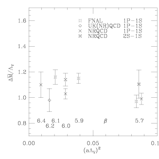
Figure 9: Asymptotic scaling plot for the quenched ${b\bar{b}}$ spectrum. Flat dependence (up to logs) on $({a\Lambda_{V}})^{2}$ indicates asymptotic scaling; linear dependence indicates O($a^{2}$) discretization errors. Simulation value of $2{\rm S}$-$1{\rm S}$ splitting has been rescaled by the experimental ratio ($1{\rm P}$-$1{\rm S}$/$2{\rm S}$-$1{\rm S}$). A perturbative correction has been applied to remove the effects of O($a^{2}$) errors in the gluonic action. Points at $\beta$=$5.7$ have been spread horizontally for clarity.

The dependence of the spin-averaged quenched ${b\bar{b}}$ splittings on $({a\Lambda_{V}})^{2}$ is shown in Fig. 9. The vertical axis is

$${\Delta{\overline{M}}\over\Lambda_{V}}=\left({(a\Delta M)_{sim}\over{a\Lambda_{V}}}\right)\left({452{\rm MeV}\over(\Delta M)_{exp}}\right),$$ (11)

where $(a\Delta M)_{sim}$ is the lattice value of the splitting being plotted, $(\Delta M)_{exp}$ is the experimental value of that splitting, and 452MeV is the experimental value of the ${b\bar{b}}$ $1{\rm P}$-$1{\rm S}$ splitting (assuming a hyperfine splitting of $50{\rm MeV}$). The rescaling by experimental values is equivalent to comparing dimensionless ratios to experiment; if two splittings have the same value of $a\Delta{\overline{M}}$, then their ratio matches experiment and they will give the same value of $a^{-1}$. I have chosen $({a\Lambda_{V}})^{2}$ as the horizontal axis because the leading discretization errors in both the FNAL and NRQCD collaboration results should be O($a^{2}$). All values were adjusted to correct for O($a^{2}$) errors in the gluonic action. All lattices have physical volume much larger than ${b\bar{b}}$ mesons.

There are three different sets of splittings in Fig. 9 (IHW and NRQCD $1{\rm P}$-$1{\rm S}$ and NRQCD $2{\rm S}$-$1{\rm S}$); all exhibit asymptotic scaling within errors. The only point that is inconsistent with flat behavior is the IHW point at $\beta$=$5.7$; both NRQCD splittings at this $\beta$ are consistent with $6.0$ (albeit with large error bars for $2{\rm S}$-$1{\rm S}$). This may be because the NRQCD collaboration removes the dominant O($a^{2}$) errors in their action ($C_{5}$ and $C_{6}$); see [9] for an estimate of the effects of these terms on the Fermilab results.

Although the results in Fig. 9 exhibit asymptotic scaling, they do not agree on $a^{-1}$! The discrepancy between $1{\rm P}$-$1{\rm S}$ and $2{\rm S}$-$1{\rm S}$ within NRQCD is good news; this is the quenching effect discussed in Fig. 6. The disagreement between NRQCD and IHW for the $1{\rm P}$-$1{\rm S}$ splitting will be bad news if it doesn’t disappear when the IHW calculation is repeated with all O($mv^{4}$) improvements turned on. If it doesn’t go away and if the scale in the NRQCD $\alpha_{s}$ calculation is 10% too high at $n_{f}$=$3$, then the value of ${\alpha_{\overline{\rm MS}}^{(5)}(M_{Z})}$ in [16] is shifted down by 2%.

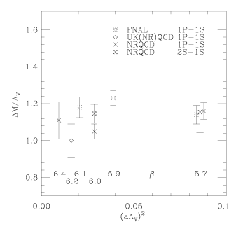
Figure 10: Same as Fig. 9, except the perturbative correction has not been applied.

At low $\beta$, there is an important caveat to the above discussion. All of the points in Fig. 9 had a perturbative correction applied to remove the effects of O($a^{2}$) errors in the gluonic ensembles[16]; the uncorrected results are shown in Fig. 10. The main effect is to move the $\beta$=$5.7$ $1{\rm P}$-$1{\rm S}$ points down significantly; the $\beta$=$5.9$ Fermilab point is also shifted down about two $\sigma$. The $2{\rm S}$-$1{\rm S}$ splitting is negligibly affected, as are ${c\bar{c}}$ splittings.

It is obviously dangerous to rely too heavily on points where this correction is large when drawing conclusions. I have chosen to apply it in these scaling plots, however, because we know that it is there and a similar calculation of the hyperfine splitting works well[16]. It is important to obtain direct results using an improved gluonic ensemble; Lepage showed in his talk that the one-loop improved gluonic action is tremendously successful at removing O($a^{2}$) errors[39]. It will be much cheaper to check asymptotic scaling in ${b\bar{b}}$ by using an improved gluonic action at $\beta$=$5.7$ than by trying to get high statistics at $\beta$=$6.4$.

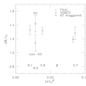
Figure 11: Same as Fig. 9, except displays quenched ${c\bar{c}}$ spectrum. All splittings shown are $1{\rm P}$-$1{\rm S}$, and have been rescaled by experimental ratio between ${b\bar{b}}$ to ${c\bar{c}}$. Gluonic correction has been applied. NRQCD point at $\beta$=$5.7$ has been moved horizontally for clarity.

Results for the $1{\rm P}$-$1{\rm S}$ splitting in ${c\bar{c}}$ are presented in Fig. 11; $2{\rm S}$-$1{\rm S}$ results are too noisy to be of interest. The discrepancy between NG and non-NG splittings in the HS formulation is obvious; the two results bracket the IHW value. There is only one $\beta$ with NRQCD results; NRQCD should blow up at $({a\Lambda_{V}})^{2}<.05$. The IHW results seem to be scaling better than for ${b\bar{b}}$; see [9] for a discussion. The high $\beta$ IHW splittings are roughly 10% higher than the low $\beta$ NRQCD splitting. I have no idea if this is related to the similar behavior in the ${b\bar{b}}$ system; O($mv^{6}$) terms left out of the NRQCD action should contribute at the 10% level for ${c\bar{c}}$. It would be very interesting to go to the next order of improvement for both the NRQCD and IHW actions in this system.

Note that $\Delta{\overline{M}}/\Lambda_{V}$ is roughly 15% larger for ${c\bar{c}}$ than for ${b\bar{b}}$. Much of this is probably due to quenching. Systematic errors in the ${c\bar{c}}$ splittings could also be noticeably contributing, however.

I combine ${c\bar{c}}$ and ${b\bar{b}}$ $n_{f}$=$2$ results in Fig. 12. Two things are striking. First, the NRQCD ${b\bar{b}}$ splittings are in much closer agreement than in Fig. 9. Again, this the same information as Fig. 6, and indicates quenching errors are being removed. Second, the NRQCD ${b\bar{b}}$ results and CDHW ${c\bar{c}}$ results disagree by roughly the same amount as in Figs. 9 and 11. This is the reason for the disagreement between the two groups’ central values of ${\alpha_{\overline{\rm MS}}^{(5)}(M_{Z})}$. Unfortunately, the KT group has much larger statistical errors. Both the CDHW and KT groups used the Wilson, rather than SW action; it would be interesting to see the CDHW run repeated using a clover, asymmetric clover, or O($mv^{4}$) IHW action.

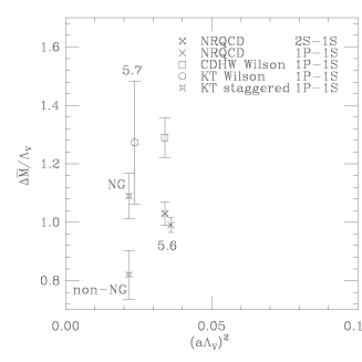
Figure 12: Same as Fig. 9, except displays $n_{f}$=$2$ spectrum. NRQCD points are ${b\bar{b}}$, all others are ${c\bar{c}}$. Splittings have been rescaled by experimental ratio. NRQCD $1{\rm P}$-$1{\rm S}$ and KT staggered points have been moved horizontally for clarity. KT staggered points are a lower bound, due to finite volume effects.

9 Conclusions

We are well on the way to having an excellent understanding of HH mesons. We already have many cross-checks; more should be forthcoming.

I wish to thank my colleagues in the Fermilab, Kyoto-Tsukuba, CDHW and NRQCD collaborations for their patience and work in supplying me with and explaining their results. This talk was prepared at the University of Glasgow, during a visit supported by the PPARC. I am extremely grateful to the members of the Physics Department there, especially Christine Davies, for their hospitality during my stay. This work was supported in part by a DOE grant.

References

- [1] G.P. Lepage et al., Phys. Rev. D46 (1992) 4052 and references therein.
- [2] A.X. El-Khadra, A.S. Kronfeld and P.B. Mackenzie, in preparation.
- [3] G.P. Lepage, Nucl. Phys. B (Proc. Suppl.) 26 (1992) 45
- [4] P.B. Mackenzie Nucl. Phys. B (Proc. Suppl.) 30 (1993) 35
- [5] C.T.H. Davies, Nucl. Phys. B (Proc. Suppl.) 34 (1994) 135
- [6] G.P. Lepage and P.B. Mackenzie, Phys. Rev. D48 (1993) 2250.
- [7] A.S. Kronfeld, Nucl. Phys. B (Proc. Suppl.) 30 (1993) 445
- [8] B. Sheikholeslami and R. Wohlert, Nucl. Phys. B 259 (1985) 572
- [9] A.X. El-Khadra, these proceedings.
- [10] S.M. Catterall et al., Phys. Lett. 321B (1994) 246.
- [11] G.T. Bodwin, S. Kim and D.K. Sinclair, Nucl. Phys. B (Proc. Suppl.) 34 (1994) 434; these proceedings.
- [12] S. Aoki et al., UTHEP-280 (1994), hep-lat-9407015.
- [13] T. Onogi et al., Nucl. Phys. B (Proc. Suppl.) 34 (1994) 492
- [14] M. Wingate et al., these proceedings.
- [15] NRQCD Collaboration: C.T.H. Davies et al., these proceedings.
- [16] C.T.H. Davies et al., OHSTPY-HEP-T-94-013 (1994) hep-ph-9408328, to appear in Phys. Lett. B.
- [17] C.T.H. Davies et al., Phys. Rev. Lett. 73 (1994) 2654.
- [18] A.S. Kronfeld and B.P. Mertens, Nucl. Phys. B (Proc. Suppl.) 34 (1994) 495
- [19] A.S. Kronfeld, these proceedings.
- [20] A.X. El-Khadra, A.S. Kronfeld, P.B. Mackenzie and B. Mertens, in progress.
- [21] C. Morningstar, Nucl. Phys. B (Proc. Suppl.) 34 (1994) 425; Phys. Rev. D48 (1993) 2265.
- [22] C. Morningstar, Phys. Rev. D50 (1994) 5902.
- [23] B. Mertens, private communication.
- [24] S. Aoki et al., these proceedings.
- [25] M. Fukugita et al., Phys. Rev. D47 (1993) 4739.
- [26] A.X. El-Khadra et al., in progress.
- [27] C.T.H. Davies et al., OHSTPY-HEP-T-94-005 (1994) hep-lat-9406017, to appear in Phys. Rev. D.
- [28] K. Bitar et al., Nucl. Phys. B (Proc. Suppl.) 26 (1992) 259; Phys. Rev. D46 (1992) 2169.
- [29] A.X. El-Khadra et al., Phys. Rev. Lett. 69 (1992) 729.
- [30] NRQCD Collaboration: G.P. Lepage et al., Nucl. Phys. B (Proc. Suppl.) 34 (1994) 417
- [31] C.T.H. Davies et al., in preparation.
- [32] S.J. Brodsky, G.P. Lepage and P.B. Mackenzie, Phys. Rev. D28 (1983) 228.
- [33] N. Gray et al., Z. Phys. C48, 673 (1990).
- [34] A.X. El-Khadra Nucl. Phys. B (Proc. Suppl.) 34 (1994) 449
- [35] C. Michael, plenary talk, these proceedings.
- [36] M. Lüscher et al.,Nucl.Phys. B359(1991)221; Nucl. Phys. B413 (1994) 481.
- [37] K.M. Bitar et al., Phys. Rev. D48 (1993) 370.
- [38] R. Sommer, plenary talk, these proceedings.
- [39] G.P. Lepage, these proceedings.