Application of the multicanonical

multigrid Monte Carlo method to

the two-dimensional $\phi^{4}$-model:

autocorrelations and interface tension

Wolfhard Janke¹ and Tilman Sauer²

¹ Institut für Physik, Johannes Gutenberg-Universität Mainz

55099 Mainz, Germany

² Institut für Theoretische Physik, Freie Universität Berlin

14195 Berlin, Germany

Abstract

We discuss the recently proposed multicanonical multigrid Monte Carlo method and apply it to the scalar $\phi^{4}$-model on a square lattice. To investigate the performance of the new algorithm at the field-driven first-order phase transitions between the two ordered phases we carefully analyze the autocorrelations of the Monte Carlo process. Compared with standard multicanonical simulations a real-time improvement of about one order of magnitude is established. The interface tension between the two ordered phases is extracted from high-statistics histograms of the magnetization applying histogram reweighting techniques.

1 Introduction

First-order phase transitions play an important role in many fields of physics [1, 2]. Examples range from the well-known process of crystal melting through the deconfining transition in hot quark-gluon matter to various steps in the evolution of the early universe. It is therefore gratifying that recently high precision Monte Carlo studies of systems undergoing a first-order phase transition have become feasible by showing that the problem of the supercritical slowing down, governed by exponentially diverging autocorrelation times

$$\tau\propto\exp\{2\sigma L^{d-1}\},$$ (1)

may be eliminated by means of the so-called multicanonical algorithm [3]. Here $\sigma$ is the interface tension between the coexisting phases, $L$ the linear size of a $d$-dimensional cubic system, and the factor $2$ accounts for the usually employed periodic boundary conditions.

While the multicanonical algorithm does beat the exponential slowing down the remaining autocorrelation times typically still diverge with some power $\alpha\approx 1\dots 1.5$ of the lattice volume $V=L^{d}$ [3, 4, 5, 6, 7, 8, 9],

$$\tau\propto V^{\alpha},$$ (2)

and may consequently still be severe. It is therefore worthwhile to look for further improvements of the Monte Carlo scheme. Critical slowing down with a power-law divergence of the autocorrelation time is a notorious problem for simulating systems at a second-order phase transition. Fortunately also here substantial progress was made in the past few years by designing modified Monte Carlo update schemes which reduce or even eliminate the critical slowing down, see Ref.[10] for reviews. Among these sophisticated Monte Carlo schemes multigrid techniques [11, 12, 13, 14, 15, 16] have been shown both to perform quite successfully and to be rather generally applicable. In a recent paper we have therefore proposed [16, 17] to combine the multicanonical approach with multigrid techniques and have presented preliminary investigations [17] which show that autocorrelation times in the multicanonical simulation may further be reduced by this combination. The purpose of this paper is to present a detailed study of the performance of the multicanonical multigrid method applied to a scalar two-dimensional $\phi^{4}$-theory on the lattice.

For Potts models it was recently proposed along other lines to combine a multicanonical demon algorithm with cluster update methods in a hybrid-like fashion [18]. Another interesting idea is to enhance the performance of Monte Carlo simulations of systems at a first-order phase transition by treating the parameter which controls the strength of the transition as a dynamical variable [19].

The outline of the paper is as follows. After defining the model and discussing its basic features in section 2 we will briefly review the characteristic properties of multicanonical reweighting and of multigrid update techniques in section 3, and show how the two Monte Carlo schemes may be combined. We further discuss the error estimates for canonical observables computed from multicanonical simulations and introduce an associated effective autocorrelation time which allows for a direct comparison with canonical simulations. Details of the calculation which in principle is straightforward but nonetheless requires some care are presented in Appendix A. In section 4 we focus on the autocorrelation times achieved by the different update algorithms. After presenting some data for the canonical case for later comparison we first analyze autocorrelations in the pure multicanonical distribution. We then discuss how the effective autocorrelation time emerges from these data. Since the multicanonical multigrid method allows to simulate the model with some accuracy, we compute in section 5 the interface tension using histogram reweighting techniques. In section 6 we conclude with some remarks on the applicability of the method and on future perspectives.

2 The model and observables

As a test case to study the performance of the recently proposed multicanonical multigrid algorithm [16, 17] we have taken the two-dimensional scalar $\phi^{4}$-model on a square $L\times L$-lattice with periodic boundary conditions. This model has been studied recently in a number of numerical investigations and has repeatedly been used as a testing ground for advanced numerical simulation techniques [11, 20, 21, 22, 23]. Previous investigations have focussed on properties of the model at criticality [22], in particular on the question of finite-size scaling and the universality with the Ising model [20, 23]. In this paper we present data from simulations performed in the broken symmetry phase, that is, strictly below the critical temperature at zero magnetic field (along the first-order transition curve). We focus on the autocorrelations of the Monte Carlo process and on the interface tension between the two ordered phases of positive and negative magnetization.

The model is defined by the partition function

$${\cal Z}(\mu^{2},g)=\prod_{i=1}^{V}\left[\int_{-\infty}^{+\infty}d\phi_{i}\right]\exp\{-{\cal H}(\{\phi_{i}\})\},$$ (3)

where

$${\cal H}(\{\phi_{i}\})=\sum_{i=1}^{V}[\frac{1}{2}(\vec{\nabla}\phi_{i})^{2}-\frac{\mu^{2}}{2}\phi_{i}^{2}+g\phi_{i}^{4}].$$ (4)

Here $(\vec{\nabla}\phi_{i})^{2}=\sum_{\mu=1}^{d}(\phi_{i_{\mu}}-\phi_{i})^{2}$ is the squared lattice gradient where $i_{\mu}$ denotes the nearest neighbor index in the lattice direction $\mu$, and $V=L^{d}$ is the volume of a $d$-dimensional cubic system. The constants $\mu^{2},g>0$ are parameters to be specified later, and the energy is measured in temperature units, i.e., we have set $\beta=1/k_{B}T=1$. Observables for the model are denoted by

$$M_{k}\equiv\sum_{i=1}^{V}\phi_{i}^{k},\quad k=1,2,\dots,$$ (5)

and the corresponding densities are denoted by $m_{i}\equiv M_{i}/V$. The kinetic term will be denoted by

$$K_{0}\equiv\sum_{i=1}^{V}(\vec{\nabla}\phi_{i})^{2}.$$ (6)

Other quantities can be defined as functions of these observables, thus the energy $E$ is given by

$$E = \frac{1}{2}K_{0}-\frac{\mu^{2}}{2}M_{2}+gM_{4},$$ (7)

and the specific heat $C$ and the (finite lattice) susceptibility $\chi$ can be obtained from

$$C = (\langle E^{2}\rangle-\langle E\rangle^{2})/V,$$ (8)

$$\chi = (\langle M_{1}^{2}\rangle-\langle|M_{1}|\rangle^{2})/V.$$ (9)

In $d=2$ dimensions the model (3,4) displays a line of second-order phase transitions in the $(\mu^{2},g)$-plane which was numerically determined in Ref.[22]. In the thermodynamic limit the system shows spontaneous symmetry breaking for all $\mu^{2}>\mu_{c}^{2}(g)$ with a nonvanishing expectation value of the average magnetization $\langle M_{1}\rangle$. Adding a term $-h\phi_{i}$ to the energy (4) the system changes discontinuously from a state of positive magnetization $\langle M_{1}\rangle>0$ to a state of negative magnetization $\langle M_{1}\rangle<0$ if we tune the magnetic field $h$ from positive to negative values. For vanishing magnetic field $h=0$, the system consequently is at a first-order phase transition. If the linear length is finite, $L<\infty$, the system then is flipping back and forth between states of positive and negative magnetization which renders $\langle M_{1}\rangle=0$ also for $\mu^{2}>\mu_{c}^{2}(g)$. At a first-order phase transition point finite systems can also exist in a mixed phase configuration which is characterized by regions of the pure phases separated by interfaces. For topological reasons there are necessarily an even number of interfaces of length $L$ for periodic boundary conditions which we have always used. For energetic reasons configurations of more than two interfaces almost never occur. A typical mixed phase configuration is shown in Fig.1. Due to the additional free energy of the interfaces, configurations with small total magnetization are suppressed by a factor $\exp(-2\sigma L)$ where $\sigma$ is the interface tension. For this reason the probability distribution of the magnetization $P(m_{1})$ shows two distinct peaks separated by a region of strongly suppressed mixed phase configurations.

Following Binder [24] one can extract the interface tension $\sigma$ by determining the ratio of the maxima $P^{\rm max}$ to the minimum $P^{\rm min}$ of the distribution $P(m_{1})$. The interface tension is then given by

$$\sigma=\lim_{L\to\infty}\sigma_{L},$$ (10)

with

$$e^{-2\sigma_{L}L}=\frac{P^{\rm min}}{P^{\rm max}}.$$ (11)

This expression can easily be evaluated provided that the statistical uncertainties of both $P^{\rm max}$ and $P^{\rm min}$ are small, which can be achieved by performing simulations according to the multicanonical distribution.

Since in this paper we study the $\phi^{4}$-model as a testing ground for the performance of Monte Carlo algorithms at first-order phase transitions the primary observable of interest will be the average magnetization $m_{1}$ and its autocorrelations in the Monte Carlo process. Although for the partition function (3,4) this observable vanishes trivially in finite systems for reasons of symmetry we emphasize that this symmetry is completely artificial and would at once be broken, e.g., by adding some term of odd power in ${\phi}$ to the energy in (4).

Autocorrelations provide a measure for the dynamics of different Monte Carlo schemes, see Ref.[25] for a review. In general, if ${\cal O}_{i}$ denotes the $i$-th measurement of an observable ${\cal O}$ in the Monte Carlo process the autocorrelation function $A(j)$ is defined by

$$A(j)=\frac{\langle{\cal O}_{i}{\cal O}_{i+j}\rangle-\langle{\cal O}_{i}\rangle^{2}}{\langle{\cal O}_{i}^{2}\rangle-\langle{\cal O}_{i}\rangle^{2}},$$ (12)

and from $A(j)$ the integrated autocorrelation time $\tau^{\rm int}$ is obtained in the large $k$ limit of

$$\tau(k)=\frac{1}{2}+\sum_{j=1}^{k}A(j).$$ (13)

Since for large $j$ the autocorrelation function $A(j)$ decays like an exponential

$$A(j)\buildrel j\rightarrow\infty\over{\longrightarrow}a\exp(-j/\tau^{\rm exp}),$$ (14)

where $\tau^{\rm exp}$ denotes the exponential autocorrelation time and $a$ is some constant, $\tau(k)$ behaves like

$$\tau(k) = \tau^{\rm int}-a\sum_{j=k+1}^{\infty}\exp(-j/\tau^{\rm exp})$$ (15)

$$= \tau^{\rm int}-a\frac{\exp\{-1/\tau^{\rm exp}\}}{1-\exp\{-1/\tau^{\rm exp}\}}\exp\{-k/\tau^{\rm exp}\},$$ (16)

where $\tau^{\rm int}\equiv\tau(\infty)$. The latter expression may be used for a numerical determination of the exponential and integrated autocorrelation times. Since, in general, all these quantities depend on the observable under consideration we will indicate the relevant observable by an additional subscript unless it is clear from the context which obserable is meant.

3 Multicanonical Monte Carlo simulations using multigrid techniques

3.1 Multicanonical simulations

The basic idea of the multicanonical approach [3, 8, 9] is to simulate an auxiliary distribution in which the mixed phase configurations have the same weight as the pure phases and canonical expectation values are recovered by reweighting. Hence the multicanonical approach is not itself a Monte Carlo update algorithm but a general reweighting prescription which allows to simulate distributions which are numerically easier to handle.

While similar ideas have been known in the literature under the name of umbrella sampling already for a long time [26] the practical relevance of multicanonical reweighting techniques for simulations of first-order phase transitions [3, 4, 5, 6, 7, 8, 9] was realized only recently [3]. The multicanonical approach may be formulated in a rather general way for a variety of applications [8] but in the context of first-order phase transitions and quantum mechanical tunneling problems [16, 17] it may simply be regarded as being basically a reweighting technique [9].

Let $m=m(\{\phi_{i}\})$ be an observable whose probability distribution in the canonical ensemble displays two strong separated peaks. In a field driven transition, as in our case, $m(\{\phi_{i}\})$ is the magnetization $m_{1}$ and the situation has also been referred to as multimagnetical simulation [5]. For a temperature driven transition the relevant observable would be the energy of the system. In the multicanonical reweighting approach we now rewrite the partition function by introducing some function $f$ as

$${\cal Z}=\prod_{i=1}^{V}\int d\phi_{i}e^{-{\cal H}(\{\phi_{i}\})-f(m)}e^{f(m)},$$ (17)

and adjust the reweighting factor $\exp(-f(m))$ in such a way that the resulting histogram of $m$ sampled according to the multicanonical probability distribution

$$p^{\rm muca}(\{\phi_{i}\}) \propto \exp[-{\cal H}(\{\phi_{i}\})-f(m)]$$ (18)

$$\equiv \exp[-{\cal H}^{\rm muca}(\{\phi_{i}\})]$$

is approximately flat. Here ${\cal H}^{\rm muca}$ is the central object of a multicanonical simulation, and plays the same role in it as ${\cal H}$ does in a canonical simulation. Canonical observables $\langle{\cal O}\rangle_{\rm can}$ can be recovered according to

$$\langle{\cal O}\rangle_{\rm can}=\frac{\langle{\cal O}w\rangle}{\langle w\rangle},$$ (19)

where $\langle\dots\rangle$ without subscript denote expectation values in the multicanonical distribution and $w\equiv\exp(f(m))$ is the inverse reweighting factor.

The multicanonical probability distribution $p^{\rm muca}$ may be updated using any legitimate Monte Carlo algorithm. The simplest choice is a local Metropolis update where we consider as usual local moves $\phi_{i_{0}}\rightarrow\phi_{i_{0}}+\Delta\phi_{i_{0}}$ at some site ${i_{0}}$ and compute the energy difference $\Delta E^{\rm muca}$ according to (18), i.e., the decision on whether a Metropolis move will be accepted or not is now to be based on the energy difference

$$\Delta E^{\rm muca}=\Delta E+f(m+\Delta m)-f(m),$$ (20)

where $\Delta E={\cal H}(\phi_{1},\phi_{2},\dots,\phi_{i_{0}}+\Delta\phi_{i_{0}},\dots,\phi_{V})-{\cal H}(\{\phi_{i}\})$ is the canonical energy difference and $\Delta m=m(\phi_{1},\phi_{2},\dots,\phi_{i_{0}}+\Delta\phi_{i_{0}},\dots,\phi_{V})-m(\{\phi_{i}\})$ is the corresponding difference in the observable $m$. If the canonical probability distribution is reweighted in the magnetization, $m(\{\phi_{i}\})=m_{1}=\sum_{i=1}^{V}\phi_{i}/V$, this difference is simply given by $\Delta m=\Delta\phi_{i_{0}}/V$. For a temperature-driven transition we have $m={\cal H}/V$ and $\Delta m=\Delta E/V$.

In practical simulations $f$ may be recorded in form of a simple stair case function which does not introduce any numerical inaccuracy since this factor cancels out in all canonical expectation values. It is also worth mentioning that since $m$ depends on all values of $\phi_{i}$, the resulting multicanonical energy is essentially nonlocal.

As we will discuss in Section 3.3, the multicanonical probability distribution $p^{\rm muca}$ may also be updated by a multigrid Monte Carlo method.

3.2 Multigrid techniques

The basic idea of multigrid Monte Carlo techniques [11, 12, 13, 14, 15, 16, 27, 28] is to systematically perform updates on different length scales of the system. In the corresponding unigrid viewpoint, which always looks at the effects on the original fine grained lattice, this is done by moving blocks of $1$, $2^{d}$, $4^{d}$, $8^{d}$, $\dots$, $2^{nd}=V$ adjacent variables at a time. In the multigrid formulation these collective update moves are implemented by introducing auxiliary fields on coarse-grained lattices. Specifically one introduces a sequence of coarsened grids $\Xi^{(k)},k=n-1,\dots,0$ of size $2^{kd}$. In the simplest piecewise constant interpolation scheme we identify a pair, square, cube, etc. of $2^{d}$ neighbouring grid points on a grid of level $k$ with a single grid point of the next coarsened grid $\Xi^{(k-1)}$. On these coarsened grids we have auxiliary fields $\phi_{i}^{(k-1)}$ representing the collective moves of the original fine-grained lattice. A (piecewise constant) interpolation operator ${\cal P}$ is defined by simply adding a finite value of some variable $\phi_{i}^{(k-1)}$ on a coarse grid to each of the $2^{d}$ corresponding grid points of the next finer grid. This allows to define a Hamiltonian of the coarse grid in terms of the Hamiltonian on the next finer grid by [11]

$${\cal H}^{(k-1)}(\{\phi_{i}^{(k-1)}\})={\cal H}^{(k)}(\{\phi_{i}^{(k)}\}+{\cal P}(\{\phi_{i}^{(k-1)}\})).$$ (21)

In essence this prescription defines a Hamiltonian on the coarse grid $\Xi^{(k-1)}$ by freezing the field variables $\phi_{i}^{(k)}$ of the next finer grid and calculating the effect of collective moves represented by the field variables $\phi_{i}^{(k-1)}$ added onto $\Xi^{(k)}$ by the piecewise constant interpolation operator. If the functional form of the Hamiltonian remains stable under the coarsening prescription [29] this multigrid implementation of the collective move updates minimizes the amount of computational effort compared to the straightforward unigrid implementation of the collective move update, in a way similar to the Fast Fourier Transformation (FFT). Also, it allows to define the multigrid update in the following recursive way. Updates of level $\Xi^{(k)}$ consist of a) $n_{1}$ presweeps using any valid local update scheme with Hamiltonian (21), b) calculating the Hamiltonian for the next coarser grid $\Xi^{(k-1)}$ (which according to (21) depends on the current configuration on grid $\Xi^{(k)}$) and initializing the variables on grid $\Xi^{(k-1)}$ to zero. One then c) updates the field variables $\phi_{i}^{(k-1)}$ by applying the multigrid update $\gamma_{k-1}$ times. To complete the update cycle one then d) interpolates the variables of grid $\Xi^{(k-1)}$back to grid $\Xi^{(k)}$ and e) performs another $n_{2}$ postsweeps of the local update algorithm. On the coarsest grid, of course, one only performs steps a) and e). In this way we cycle through the sequence of coarsened grids in a specific manner which is determined by the parameters $\gamma_{k}$. Particularly successful is the choice $\gamma_{k}\equiv 2$, a sequence which is commonly called W-cycle since its graphical representation very much resembles the letter W.

3.3 Multicanonical multigrid Monte Carlo

From the unigrid viewpoint it is immediately clear that the multicanonical and multigrid methods can easily be combined for a field-driven transition where $m=m_{1}$ is the average magnetization [16, 17]. Since on level $k$ we effectively always move $2^{(n-k)d}$ spins in conjunction an accepted Metropolis move would change the average field $m_{1}$ by an amount of $2^{(n-k)d}\Delta\phi^{(k)}_{i_{0}}/V$. The only modification for the update on level $k$ will therefore be to compute the energy difference according to

$$\Delta E^{{\rm muca},(k)}=\Delta E^{(k)}+f(m+2^{(n-k)d}\Delta\phi_{i_{0}}^{(k)}/V)-f(m),$$ (22)

where $\Delta E^{{\rm muca},(k)}$ is the energy difference computed with the coarse-grid Hamiltonian (21) as in the usual canonical multigrid formulation. While this modification is obvious from the unigrid point of view it should be stressed that the modifications for a recursive multigrid implementation are precisely the same.

In our case the doubly peaked observable $m$ which controls the multicanonical reweighting factor is the magnetization $m_{1}$. In this case the necessary modifications for a recursive multigrid update of the multicanonical Hamiltonian ${\cal H}^{\rm muca}$ are in fact almost trivial. The combination of multigrid update schemes with the multicanonical reweighting idea, however, is neither restricted to the special choice of $m=m_{1}$ nor to any special choice of the reweighting factor $f$. In general, a multigrid Monte Carlo update of a multicanonical Hamiltonian ${\cal H}^{\rm muca}(\{\phi_{i}\})={\cal H}(\{\phi_{i}\})+f(m(\{\phi_{i}\}))$ should be feasible and effective whenever both the canonical Hamiltonian ${\cal H}$ and the parameter $m$ are stable under coarsening. To see this, let us assume we would want to reweight the canonical Hamiltonian ${\cal H}$ in some other observable of $\{\phi_{i}\}$, say $m=m_{2}$, rather than in $m=m_{1}$. In order to compute the reweighting factor $f(m_{2})$ on level $k$ we would need to know the actual value of $m_{2}$ as a function of the coarse-grid variables $\phi^{(k)}_{i}$. Clearly, we cannot simply compute the average value of $m_{2}$ by multiplying $\Delta\phi_{i_{0}}^{(k)}$ with a simple factor as was the case for the average magnetization. Indeed, from the unigrid point of view we would need to know the actual configuration of the original-grid variables and the efficiency gained from the multigrid update would be lost at least for this part of the update. It is therefore important to realize that $m_{2}$ may also be calculated using the usual coarsening prescription. In general, the analog of eq. (21) for the function $m$ would simply read

$$m^{(k-1)}(\{\phi_{i}^{(k-1)}\})=m^{(k)}(\{\phi_{i}^{(k)}\}+{\cal P}(\{\phi_{i}^{(k-1)}\})).$$ (23)

Therefore we would only have to compute the coarse-grid coefficients for the function $m^{(k-1)}$ in addition to those for ${\cal H}^{(k-1)}$ and we could then use the value of $m^{(k-1)}$ in order to compute the reweighting factor. From this point of view, the factors $2^{(n-k)d}$ appearing in eq. (22) are nothing but the coarse-grid coefficients for the average magnetization using piecewise constant interpolation.

We would like to stress again at this point that the condition that $m$ remains stable under coarsening is the only restriction for an effective multigrid Monte Carlo update of a multicanonical Hamiltonian. In particular, this means that a) the reweighting factor $f(m)$ may be computed for any function $f$. In fact, the step functions normally employed are examples for rather special, highly non-linear functions. b) The condition also allows a combination of multigrid techniques and multicanonical reweighting if we take the canonical Hamiltonian ${\cal H}$ itself as the observable $m$. This would be the situation for a temperature-driven first-order transition. If ${\cal H}$ is stable under coarsening (as we always assume it is) it therefore immediately follows that a multicanonical multigrid Monte Carlo simulation would be perfectly feasible in this case as well. c) We also believe, that multicanonical multigrid Monte Carlo simulations should be feasible for models other than those characterized by a Hamiltonian of the form (4) such as non-linear O(n) sigma-models. If, e.g., one would want, for some reason, to simulate an $XY$-model with a multicanonical reweighting factor $f=f(s_{x})$ where $s_{x}$ is the average $x$-component of the spins one might express $s_{x}$ as $(\sum_{i}\cos(\Theta_{i}))/V$ and the latter function is stable under coarsening for piecewise constant interpolation if we allow for an additional term $(\sum_{i}\sin(\Theta_{i}))/V$ on the coarsened grids. More realistic but nevertheless feasible as well would be the case where the reweighting variable is the squared magnetization [30]. d) Furthermore, the fact that we only need to know the actual value of $m$ for each coarse-grid update and the fact that this value may be computed from eq. (23) also entails that the multicanonical multigrid Monte Carlo method is, in general, not restricted to the piecewise constant interpolation scheme. e) Finally, it should be recalled that multigrid techniques are sophisticated update schemes which do not presuppose specific update algorithms. In principle, we may therefore use any other valid update algorithm on the coarsened grids instead of the Metropolis update.

In this paper we will substantiate our claim that multicanonical multigrid Monte Carlo simulations are both feasible and profitable by a careful analysis of the performance of the method for the model (3), (4). For other situations the method should be tested by explicit simulations. As long as the central condition for the multicanonical multigrid approach is fulfilled, however, we do not expect any difficulties regarding the feasibility of the method.

3.4 Effective autocorrelation time

Before discussing our results it is worthwhile to comment on a technical complication which arises in evaluating the efficiency of multicanonical simulations. In previous investigations it was the exponential autocorrelation time measured in the multicanonical distribution which was used to estimate the performance of the multicanonical algorithm. Alternatively, autocorrelations were also measured by counting the average number of sweeps needed to travel from one peak maximum to the other and back (see section 4.1. below). This nicely illustrated the absence of an exponential slowing down [3, 4, 5, 6, 7, 8, 9]. It should be stressed, however, that neither the exponential autocorrelation time nor the diffusion time can a priori serve as a fair quantitative measure for comparison of the performance of multicanonical simulations with canonical update schemes. The reason is that the estimator $\hat{{\cal O}}=\sum_{i=1}^{N_{m}}{\cal O}_{i}w_{i}/\sum_{i=1}^{N_{m}}w_{i}$ of canonical observables (19) is a ratio of two different multicanonical observables which may have different autocorrelations and, moreover, are usually strongly cross-correlated. It is thus not immediately obvious how autocorrelations relevant for canonical quantities should be defined and measured in multicanonical simulations. For a fair comparison with canonical simulations we therefore define [17] an effective autocorrelation time $\tau^{\rm eff}$ and write the error estimate also in the multicanonical case in the standard form

$$\epsilon^{2}_{\hat{{\cal O}}}=(\sigma^{2}_{{\cal O}_{i}})^{\rm can}\frac{2\tau^{\rm eff}_{{\cal O}}}{N_{m}},$$ (24)

where $N_{m}$ is the number of multicanonical measurements and $(\sigma^{2}_{{\cal O}_{i}})^{\rm can}$ is the variance of ${\cal O}_{i}$ in the canonical ensemble computed according to eq.(19). A simple and numerically stable way to obtain an estimate for the effective autocorrelation time $\tau^{\rm eff}_{{\cal O}}$ is to compute the error $\epsilon^{2}_{\hat{{\cal O}}}$ of the estimator $\hat{{\cal O}}$ by jackknife blocking. In principle, $\tau^{\rm eff}_{{\cal O}}$ can also be calculated by applying standard error propagation starting from the basic reweighting formula (19). As shown in Appendix A the squared canonical error $\epsilon^{2}_{\hat{{\cal O}}}$ of the canonical estimator $\hat{{\cal O}}$ of an observable $\langle{\cal O}\rangle_{\rm can}$ based on $N_{m}$ multicanonical measurements is then given by

$$\epsilon^{2}_{\hat{{\cal O}}}= \langle{\cal O}\rangle^{2}_{\rm can} [\frac{\langle{\cal O}_{i}w_{i};{\cal O}_{i}w_{i}\rangle}{\langle{\cal O}_{i}w_{i}\rangle^{2}}\frac{2\tau^{\rm int}_{{\cal O}w;{\cal O}w}}{N_{m}}+\frac{\langle w_{i};w_{i}\rangle}{\langle w_{i}\rangle^{2}}\frac{2\tau^{\rm int}_{w;w}}{N_{m}}$$ (25)

$$-2\frac{\langle{\cal O}_{i}w_{i};w_{i}\rangle}{\langle{\cal O}_{i}w_{i}\rangle\langle w_{i}\rangle}\frac{2\tau^{\rm int}_{{\cal O}w;w}}{N_{m}}].$$

where $\langle x;y\rangle\equiv\langle xy\rangle-\langle x\rangle\langle y\rangle$ is the covariance matrix of two observables $x$ and $y$. From this expression it is clear that in general three different integrated autocorrelation times $\tau^{\rm int}_{{\cal O}w;{\cal O}w}$, $\tau^{\rm int}_{w;w}$, and $\tau^{\rm int}_{{\cal O}w;w}$ of the observables ${\cal O}w$ and $w$ (measured in the multicanonical distribution) must be taken into account.

4 Results

We have simulated the model (3,4) in two dimensions ($d=2$) at three different points in the ($\mu^{2},g$)-plane, namely we have taken $g=0.25$ and varied $\mu^{2}$ as $\mu^{2}=1.30,1.35$, and $1.40$. For this value of $g$, the second-order phase transition to the disordered phase occurs at $\mu^{2}_{c}=1.265(5)$ as it was determined in Ref. [22], confirmed in Ref. [23], and reproduced in our own simulation (see section 5). With this choice of parameters our simulations were performed in a regime which shows the typical first-order behavior already for relatively small lattices. For large linear lattice size $L$ the ratio between the maxima and the minima of the histogram for $m_{1}$ will then easily take on several orders of magnitude. For the severest case which we have investigated ($\mu^{2}=1.40,L=64$) this ratio, e.g., is already more than 9 orders of magnitude. In these extreme cases an important point of the multicanonical algorithm is the way to obtain the trial histogram since the performance of the multicanonical simulation strongly depends on the quality of the assumed trial distribution. If there is no chance to make an initial guess on the basis of some knowledge of the system, the most straightforward way to proceed is by iterations which in our case was done as follows. Starting with a canonical simulation we performed some thermalizing sweeps and then obtained a first histogram on the basis of $50\,000\times n_{e}$ sweeps. Here $n_{e}$ is a parameter which allows to adjust the time scale of the MC process, i.e., measurements were always taken only after every $n_{e}$ “empty” sweeps. In the multigrid case we count a complete cycle as one sweep, and we only performed presweeps, i.e., we always had $n_{1}=1$ and $n_{2}=0$. In order to maintain a roughly constant Metropolis acceptance rate of about $50$% we had to scale down the maximal step width $\propto 0.6^{n-k}$ which conforms with recent analytical investigations of the Metropolis acceptance rate [31]. The first histogram was then symmetrized and any empty bins between the peaks were filled by interpolation using rough estimates for the interface tension obtained from simulations of the smaller lattices. Using this histogram as a first guess to construct the reweighting factor $\exp(-f)$ we performed another $50\,000\times n_{e}$ multicanonical sweeps. The resulting histogram proved to be sufficient for lattice sizes $L=8,16$, and $32$. To obtain high precision the resulting histogram nevertheless was in any case again symmetrized and taken for the final simulation run. For $L=64$ we have done one more iteration of $1\,000\,000\times n_{e}$ sweeps and used only this resulting histogram as trial distribution for the final run. For the determination of the trial histograms, which always had a bin size of $0.008$, we have in any case used the W-cycle and, to allow for a direct comparison, we have taken the same trial histograms for the final runs of both the standard multicanonical simulation and the combination with the multigrid scheme. In our final runs we have in each case performed $1\,000\,000\times n_{e}$ sweeps after discarding $10\,000\times n_{e}$ sweeps for thermalization. To allow for later histogramming and flexible analysis of autocorrelations we have recorded the time series of $K_{0}$, $M_{1}$, $M_{2}$, and $M_{4}$, and all errors were computed by jackkniving [32] the data with 50 blocks.

Figures 2(a-c) show the flat multicanonical distributions and the canonical double-peak histograms of $m_{1}$ after reweighting for $\mu^{2}=1.30$ and different lattice sizes $L=8,16$, and $32$. The quality of the flatness of the multicanonical distributions for our largest lattices ($L=64$) and for $\mu^{2}=1.30,1.35$, and $1.40$ can be judged from Figs. 3(a-c). Although the multicanonical distributions are essentially flat between the peaks there still is some structure in the multicanonical distributions which affects autocorrelations of $m_{1}$. Note the flat regions in the canonical histograms for $m_{1}\approx 0$ which reflect the fact that mixed phase configuration for some range of $m_{1}$ all look similar to the one displayed in Fig. 1. Different total magnetizations in this regime result from a relative shift of the two interfaces and the free energy of these configurations is the same as long as interactions between the interfaces are negligible. The arrow in Fig. 3c indicates the value of $m_{1}$ for the configuration displayed in Fig. 1.

The drastic difference between the canonical and the multicanonical updates can be illustrated by looking at the time series of $m_{1}$ as shown in Figs. 4 (a-d). While the time series in the canonical case clearly displays the instantons characteristic for tunnelling processes the observable in the multicanonical simulation shows a random walk like behavior. In either case the use of the multigrid update affects the time scale of the autocorrelations. Note that the time scale in the figures has been adjusted in such a way that they display the time evolution over a length of roughly $30\times\tau^{\rm int}_{m_{1}}$ in either case (cp. Tables 1 and 2 below).

To get a more precise view of the performance of the different Monte Carlo schemes we have measured autocorrelation times of the relevant observables. In order to obtain estimates for the integrated autocorrelation time $\tau^{\rm int}$ a common way to proceed is to cut the sum (13) self-consistently at $k=n_{\rm cut}\times\tau^{\rm int}$ where $n_{\rm cut}$ is usually chosen to be $6$ or $8$. As long as $\tau^{\rm int}\approx\tau^{\rm exp}$ this method usually gives sufficiently reliable values. If, however, $\tau^{\rm exp}$ is appreciably larger than $\tau^{\rm int}$ this method systematically underestimates the integrated autocorrelation time. Let us illustrate the problem for the rather extreme case of ${\cal O}=m_{1}\exp(f)$, $\mu^{2}=1.40$, and $L=64$, cp. Fig.5. Here we find an exponential autocorrelation time $\tau^{\rm exp}=3330(530)$ (in units of cycles) which is more than $4$ times larger than the true integrated autocorrelation time $\tau^{\rm int}=778(63)$ (cp. Table 3 below). Computing the integrated autocorrelation time by self-consistently cutting the sum in eq. (13) therefore underestimates $\tau^{\rm int}$ to be $505(15)$ for $n_{\rm cut}=6$ and $627(25)$ for $n_{\rm cut}=8$. In order to circumvent this problem we have therefore proceeded as follows (see Fig. 5). For the exponential autocorrelation time $\tau^{\rm exp}$ we have first obtained a rough guess $\tau^{{\rm exp},(0)}$ by a linear fit of $\ln A(j)$ from $j=\tau^{\rm int}\ldots 3\tau^{\rm int}$ where $\tau^{\rm int}$ is the integrated autocorrelation time obtained by cutting eq.(13) self-consistently with $n_{\rm cut}=8$. The inset in Fig. 5 shows a logarithmic plot of the autocorrelation function $A(j)$ for the example discussed above together with this first rough guess shown by the dashed line. Clearly $A(j)$ does not behave like a single exponential as would be the case if $\tau^{\rm int}=\tau^{\rm exp}$ and consequently one must be careful to fit $\ln A(j)$ sufficiently far away from the origin. For our first approximation we obtained in this case $\tau^{{\rm exp},(0)}=2480$. We have then performed a three-parameter fit of $\tau(k)$ according to eq.(16) in the range $k=\tau^{{\rm exp},(0)}\ldots 3\tau^{{\rm exp},(0)}$ which yielded the values for $\tau^{\rm int}$ and $\tau^{\rm exp}$ quoted in Tables 1-4. Fig. 5 shows $\tau(k)$ and the corresponding fit. The horizontal lines represent our value of $\tau^{\rm int}$ together with its error bounds and one clearly sees that $\tau(k)$ saturates towards this values for $k\rightarrow\infty$. Again we see that the data do not yet saturate for $k=6200\approx 8\tau^{\rm int}$. The solid line in the inset shows a linear fit of $\ln A(j)$ in the same range $j=\tau^{{\rm exp},(0)}\ldots 3\tau^{{\rm exp},(0)}$. This fit yields a value $\tau^{\rm exp}=2780(670)$ which is consistent with the one we quote but has larger error bounds. Summing up, we note that fitting $\tau(k)$ according to eq.(16) rather than fitting $\ln A(j)$ produces simultaneously unbiased values for both $\tau^{\rm exp}$ and $\tau^{\rm int}$ with smaller statistical uncertainties. Also these fits were satisfactorily stable against variations of the fitting range. As usual, error bars for the values of $\tau^{\rm int}$ and $\tau^{\rm exp}$ obtained by this fitting procedure were obtained using the jackknife method.

4.1 Autocorrelations in canonical simulation

For later comparison with the multicanonical case we have first performed a number of canonical simulations using both the standard local single-hit Metropolis update and the multigrid W-cycle. Since the main focus of this paper, however, was to investigate the improvement gained by combining the multicanonical approach with multigrid techniques, standard canonical simulations were done only for $\mu^{2}=1.30$ and only for small lattices ($L=4,8,16$). Table 1 shows the measured autocorrelation times for ${\cal O}=m_{1}$ and $m_{2}$ (always given in units of sweeps resp. cycles). For ${\cal O}=m_{1}$ we see that within the error bars the integrated autocorrelation times do not differ from the exponential autocorrelation times, i.e., in this case we are dealing with an almost purely exponential autocorrelation function (see below for a theoretical explanation of this behavior). For the even observable ${\cal O}=m_{2}$ we find on the other hand that the exponential autocorrelation time $\tau^{\rm exp}$ is appreciably larger than the integrated autocorrelation time $\tau^{\rm int}$. The difference between $\tau^{\rm int}$ and $\tau^{\rm exp}$ increases on larger lattices. Comparing the improvement of using multigrid techniques with a W-cycle gives a factor of roughly $10\sim 20$. An improvement of this order had already been found in Ref.[11] for simulations at the critical line. In either case the autocorrelation times, however, diverge exponentially with increasing linear lattice size $L$.

To obtain a rough estimate of the order of magnitude of the quantities involved we have fitted the integrated autocorrelation times of $m_{1}$ according to $\tau^{\rm int}={\rm const}\times L^{\alpha}\exp(2\sigma L)$. We find $\tau^{\rm int}=6.41\times L^{2.13}\exp(2\times 0.027L)$ for the Metropolis case and $\tau^{\rm int}=4.83\times L^{0.24}\exp(2\times 0.10L)$ for the W-cycle. Since we expect that the exponent should depend on the interface tension we have also performed a constrained fit using for $\sigma$ the value for the interface tension obtained from our multicanonical simulations ($\sigma=0.03443$, see below). For this fit we find $\tau^{\rm int}=7.30(36)\times L^{2.01(22)}\exp(2\sigma L)$ for the Metropolis case and $\tau^{\rm int}=1.638(52)\times L^{1.366(16)}\exp(2\sigma L)$ for the W-cycle. Clearly, these fits can only give a rough estimate of the magnitude of the relevant quantities for two reasons. First we have only three data points for fitting two resp. three parameters. Second, we expect corrections to be still appreciable at least for the smallest lattice used ($L=4$). Nevertheless, comparable numbers were found for the two-dimensional Ising model where in [5] a behavior of $\tau^{\rm int}=6.80L^{2.14}\exp(2\times 0.185\times L)$ was found for the canonical heatbath. For the $7$-state Potts model fits of the form $1.01L^{2.31}\exp(2\times 0.01174\times L)$ have been reported in Ref. [18].

The dynamical origin of the autocorrelation time for $m_{1}$ may be illustrated by a simple two-state flip model. We measured the mean time of staying in one of the potential wells by digitalizing the evolution series corresponding to a simple two-state model with single flip dynamics [33]. This procedure is illustrated for the time series in Figs. 4a and 4c. Counting the number of Monte Carlo time steps that the systems needs to flip from one state to the other we measure an average flip rate. A theoretical analysis of this single flip dynamics shows that the exponential autocorrelation time for this model is given by $\tau^{\rm flip}$ where $4\tau^{\rm flip}$ is the average time the system needs to flip from one state to the other and back. The measured flipping times are also shown in Table 1. For large $\tau^{\rm flip}$ the variance $\sigma^{2}$ of $\tau^{\rm flip}$ is given by $(\tau^{\rm flip})^{2}$ itself as can be calculated in the single flip dynamics and as we have verified in our canonical simulations. The error bars for the flipping times $\tau^{\rm flip}$ therefore were calculated as $\delta\tau^{\rm flip}=\tau^{\rm flip}/\sqrt{n_{e}}$ where $1/n_{\rm flip}$ is the measured total flip rate, i.e. $2\tau^{\rm flip}n_{\rm flip}=N_{m}\times n_{e}$. As can be seen in Table 1 application of the multigrid algorithm speeds up the Monte Carlo process by increasing the average flip rate by a roughly constant factor.

4.2 Autocorrelations in multicanonical simulation

In the multicanonical simulation the exponential supercritical slowing down is overcome by simulating an auxiliary distribution which is flat between the two maxima of the histogram, cp. Figs. 2 and 3, and in this case we expect the autocorrelations to be governed by some random walk dynamics, cp. Figs. 4b and 4d. Since multigrid techniques can be applied in the multicanonical distribution as well it is of interest to see whether a further reduction of autocorrelations can be achieved by this combination. From the rather different scales of Figs. 4b and 4d it is already clear qualitatively that autocorrelations are in fact reduced. In order to see quantitatively how multicanonical simulations are improved by multigrid updating we first measured autocorrelations of the corresponding observables in the multicanonical distribution using both the standard single-hit Metropolis algorithm and the W-cycle. Table 2 shows our results for this case. We see that for ${\cal O}=m_{1}$ it is again found that $\tau^{\rm int}_{m_{1}}\approx\tau^{\rm exp}_{m_{1}}$, i.e., also in the multicanonical dynamics the autocorrelation function decays like a pure exponential. For the even observable ${\cal O}=m_{2}$, on the other hand, there is again a difference between integrated and exponential autocorrelation times.

Comparing the absolute values for the Metropolis update and for the W-cycle we find that for both observables the multigrid method reduces the autocorrelation times by a factor of roughly $15\approx 20$.

We have also looked at the lattice size dependence of the autocorrelation times by fitting the data for ${\cal O}=m_{1}$ according to $\tau^{\rm int}=a_{\rm int}L^{z_{\rm int}}$ or $\tau^{\rm exp}=a_{\rm exp}L^{z_{\rm exp}}$ (where $z=\alpha d$). Here we first note that trivially the exponent $z_{\rm int}$ for the integrated autocorrelation times agrees with the exponent $z_{\rm exp}$ for the exponential autocorrelation times. We also find that fitting only the data for $L=8,16$, and $32$ yields approximately the same exponents for the Metropolis case and for the multigrid W-cycle. Looking at the dependence on the parameter $\mu^{2}$ we find that the exponent increases with $\mu^{2}$, i.e. with the strength of the transition. Fitting the integrated autocorrelation times obtained from the multigrid simulation for lattice sizes, $L=16,32$, and $64$, we obtain exponents of about $2.2$, $2.5$, and $2.7$ for $\mu^{2}=1.30$, $1.35$, and $1.40$. Including the $L=8$-data worsens the fits, and we therefore believe that for a reliable estimate one would need to include even larger lattices. In general, we observe that the fits have rather large chi-squares, and we hesitate to draw any definite conclusions. The deviations from linearity found in the log-log-fits are believed to be effected by the fact that the multicanonical histograms are not ideally flat. In Figs. 2 (a-c) and 3 (a-c) the multicanonical histograms look better than they actually are as a result of the logarithmic scale. On a linear scale one still discerns some structure in the supposedly flat region between the peaks at least for the larger lattices. Therefore the statistical accuracy of our data seems to be better than the systematic fluctuations of the autocorrelation times caused by imperfect multicanonical trial histograms.

With respect to the purely multicanonical dynamics, we conclude that the multigrid technique does not affect the exponent $z=\alpha d$. However, it is by largely reducing the overall scale of the autocorrelation, i.e. by reducing the prefactor $a$, that application of multigrid techniques gives an improvement factor of roughly $15\sim 20$, i.e. of about one order of magnitude. The improvement factor shows a weak tendency to increase if $\mu^{2}$ approaches the critical value.

4.3 Effective canonical autocorrelations in multicanonical simulation

Clearly, the multicanonical reweighting factor is an algorithmical artefact introduced in order to obtain higher statistical accuracy for the measurement of canonical observables. For a fair comparison between the canonical and the multicanonical simulation we therefore have to estimate the error bars associated with the canonical observables.

Odd observables:

For odd observables standard error propagation starting from eq.(19) shows that the effective autocorrelation time $\tau^{\rm eff}_{{\cal O}}$ for canonical estimates obtained by measurements in the multicanonical distribution is given by

$$\tau_{{\cal O}}^{\rm eff}=\frac{\sigma^{2}_{\hat{{\cal O}}}}{(\sigma_{{\cal O}_{i}}^{2})^{\rm can}}\tau_{{\cal O}w;{\cal O}w},$$ (26)

(see Appendix A) with the effective multicanonical variance

$$\sigma^{2}_{\hat{{\cal O}}}=\langle{\cal O}\rangle^{2}_{\rm can}\frac{\langle{\cal O}_{i}w_{i};{\cal O}_{i}w_{i}\rangle}{\langle{\cal O}_{i}w_{i}\rangle^{2}}=\frac{\langle{\cal O}_{i}w_{i};{\cal O}_{i}w_{i}\rangle}{\langle w_{i}\rangle^{2}}.$$ (27)

Table 3 shows the measured integrated and exponential autocorrelation times $\tau^{\rm int}$ and $\tau^{\rm exp}$ for ${\cal O}=m_{1}\exp(f)$. Also shown are the effective multicanonical variance $\sigma^{2}_{\hat{\cal O}}$ according to eq.(27), the canonical variance $(\sigma^{2}_{{\cal O}_{i}})^{\rm can}$ of ${\cal O}=m_{1}$, which can be computed in a multicanonical simulation by using eq.(19), the effective autocorrelation time $\tau^{\rm eff}_{m_{1}}$ computed according to eq.(26), and the diffusion time $\tau^{\rm flip}_{m_{1}}$ defined in analogy to section 4.1.

First, we notice that, within error bounds, the exponential autocorrelation times for ${\cal O}=m_{1}\exp(f)$ agree with the purely multicanonical autocorrelation times for ${\cal O}=m_{1}$ listed in Table 2. This is not surprising since we are still dealing with an odd observable whose slowest autocorrelation mode should be same. The integrated autocorrelation times on the other hand in this case differ appreciably. This is an indication that the autocorrelation function (12) does not behave like a simple exponential $\propto\exp(-j/\tau^{\rm exp})$. Rather it is composed of many different modes with only the slowest mode decaying with $\tau^{\rm exp}$ as illustrated in the inset of Fig. 5. The relative difference between the integrated and the exponential autocorrelation time increases both with the size of the system and with $\mu^{2}$. The ratio does not depend on the other hand on the use of the algorithm, being roughly the same both for the standard Metropolis update and for the multigrid update.

Table 3 lists both the effective multicanonical and the canonical variances. These allow to compute the final effective autocorrelation times which are also reported. While the canonical variance depends only weakly on the size of the system the effective multicanonical variance $\sigma^{2}_{\hat{{\cal O}}}$ varies appreciably with the linear lattice size $L$. In the worst case, $\mu^{2}=1.40$ and $L=64$ the ratio is already $\sigma^{2}_{\hat{{\cal O}}}/(\sigma^{2}_{{\cal O}_{i}})^{\rm can}\approx 11$. Consequently the effective autocorrelation time which should be used for comparisons with canonical algorithms is much larger than the simple exponential autocorrelation time $\tau^{\rm exp}$.

To allow for further comparison with the literature, we have looked also for this situation at the exponents $z_{\rm int}$ resp. $z_{\rm exp}$ of the power-like divergence $\tau=aL^{z}$. In contrast to the purely multicanonical case the exponents $z_{\rm int}$ here differ from the exponents $z_{\rm exp}$. While the exponents $z_{\rm exp}$ for ${\cal O}=m_{1}\exp(f)$ roughly agree with those for the purely multicanonical observable ${\cal O}=m_{1}$ and thus increase with $\mu^{2}$, the exponents $z_{\rm int}$ seem to stay constant with increasing $\mu^{2}$. Finally we note that the exponent $z_{\rm eff}$ for the effective autocorrelation time $\tau^{\rm eff}$ again increases with $\mu^{2}$ which directly reflects the scaling of the ratio $\sigma^{2}_{\hat{{\cal O}}}/(\sigma^{2}_{{\cal O}_{i}})^{\rm can}$ with $\mu^{2}$ and $L$. The increase of $z_{\rm eff}$ with $\mu^{2}$ as compared to $z_{\rm int}$ is illustrated in Fig. 6. Here the integrated autocorrelation times $\tau^{\rm int}$ for ${\cal O}=m_{1}\exp(f)$ are shown together with the corresponding effective autocorrelation times $\tau_{\rm eff}$. The straight lines show fits of the form $\tau^{\rm int}=a_{\rm int}L^{z_{\rm int}}$ and $\tau^{\rm eff}=a_{\rm eff}L^{z_{\rm eff}}$. From this figure it can also be seen that the data for the smallest lattice, $L=8$, need still be excluded to obtain satisfactory fits. Fitting the data for $L=16,32$, and $64$ we find for the effective exponents $z_{\rm eff}$ values of about $2.3$, $2.7$, and $3.0$ for $\mu^{2}=1.30$, $1.35$, and $1.40$. The exponents obtained in our work confirm qualitatively the exponents found for standard multicanonical simulations of the two-dimensional $q$-state Potts model where exponents of $z=2.65(5)$ for $q=7$ [4] and $z=2.65(2)$ for $q=10$ [3] have been obtained from analyses of the diffusion times. Note that for a random walk like behavior as in the multicanonical case one cannot unambiguously identify distinct states anymore. One often employed possibility is to measure the average number of multicanonical sweeps or multigrid cycles needed to travel from one (canonical) peak maximum to the other and back. In analogy to the definition for canonical simulations the $\tau^{\rm flip}_{m_{1}}$ given in Table 3 are one quarter of this average travel time. By using this definition of $\tau^{\rm flip}_{m_{1}}$ we obtain a nice agreement with $\tau^{\rm eff}_{m_{1}}$ at least for the large lattices. A priori, however, other definitions of $\tau^{\rm flip}$ are reasonable as well (e.g., using $\langle|m_{1}|\rangle_{\rm can}$ for the cuts instead of the peak locations), and it is difficult to argue which one should give the best quantitative agreement with the unambiguously defined effective autocorrelation time $\tau^{\rm eff}$. For this reason a direct measurement of $\tau^{\rm eff}$ is to be preferred rather than any analogue of the two-state flip model.

For odd observables the distinction between the directly measured integrated autocorrelation time and the effective autocorrelation time does not pertain to the comparison between the standard multicanonical Metropolis update and combination of the multicanonical approach with multigrid techniques. Since the multicanonical approach is a mere reweighting technique $\sigma^{2}_{\hat{{\cal O}}}$ and $(\sigma^{2}_{{\cal O}_{i}})^{\rm can}$ are not affected by applying different update algorithms. Hence we find indeed that the same improvement factors of about $15\sim 20$ are gained both for the integrated autocorrelations and for the effective autocorrelation times. These effective improvement factors are slightly smaller than those found for ${\cal O}=m_{1}$ from Table 2 and again show a tendency to increase when $\mu^{2}$ approaches the critical value.

Even observables:

For even observables we cannot exploit the fact that $\langle{\cal O}_{i}w_{i}\rangle$ vanishes identically for reasons of symmetry in order to simplify the error propagation formula (25). In general, to obtain estimates for the canonical error of an observable ${\cal O}$ we therefore have to take recourse to the full expression of error propagation (25). Table 4 shows our results for the even observable ${\cal O}=m_{2}$ from our simulations at $\mu^{2}=1.30$. Here we list measured values for all quantities which enter the error propagation formula (25). The mean values, variances, and covariance, for the Metropolis case and for the W-cycle, are consistent within error bars, as, of course, should be the case since these quantities do not depend on the update algorithm. The integrated autocorrelation times, however, again differ by a factor of roughly $20$. We did not list the corresponding exponential autocorrelation times since these agree, within error bounds, with the exponential autocorrelation times for ${\cal O}=m_{2}$ listed in Table 2. We have also checked that $\tau^{\rm int}_{{\cal O}w;w}\approx\tau^{\rm int}_{w;{\cal O}w}$ as would be expected because of time reversal invariance.

Next to these values we then list in Table 4 the squared statistical error $\epsilon^{2}$ for the canonical estimator of ${\cal O}=m_{2}$ calculated by error propagation from the data listed before. Note that the error of this error, however, as well as all the errors given in the Table were not computed by error propagation but, as usual, calculated directly by jackkniving.

Clearly, it is this statistical error for the canonical estimates of the observable which one wants to reduce by sophisticated Monte Carlo methods. When interpreting the statistical errors reported in Table 4 the time scale set by $n_{e}$ should also be taken into consideration. While the squared errors $\epsilon^{2}$ are approximately of the same order for the Metropolis (M) update and for the multigrid W-cycle update (W) we also had to perform many more Metropolis updates since we had adjusted $n_{e}$. If, e.g., for $L=8$ the statistical error for the Metropolis update is only twice as large as the one for the multigrid update, we also had $n_{e}=5$(M) resp. 1(W), cp. Table 2. Therefore the improvement is given by $(0.540/0.2442)\times 5\approx 11$ which is roughly of the same size as the ratio of the measured autocorrelation times.

Another technical remark is due at this point. Applying formula (25) to calculate the canonical error of multicanonical measurements we run into a nasty problem of numerical cancellation. To illustrate this cancellation problem let us look at the data for $L=64$. Here we find for the first two terms in eq.(25)

$$\frac{\langle{\cal O}_{i}w_{i};{\cal O}_{i}w_{i}\rangle}{\langle{\cal O}_{i}w_{i}\rangle^{2}}\tau^{\rm int}_{{\cal O}w;{\cal O}w}+\frac{\langle w_{i};w_{i}\rangle}{\langle w_{i}\rangle^{2}}\tau^{\rm int}_{w;w}=1006.22$$ (28)

and for the third term

$$2\frac{\langle{\cal O}_{i}w_{i};w_{i}\rangle}{\langle{\cal O}_{i}w_{i}\rangle\langle w_{i}\rangle}\tau^{\rm int}_{{\cal O}w;{\cal O}w}=1006.32,$$ (29)

i.e., we have a numerical cancellation up to the fifth digit. Also if we look at $\sigma^{2}_{\hat{{\cal O}}}$ we find the same problem which should not come as a surprise if we recall that in the definition (A10) of $\sigma^{2}_{\hat{{\cal O}}}$ we simply dropped the $\tau$’s in eq.(25). Since from Table 4 we see that for the even observable $m_{2}$ we always have $\tau^{\rm int}_{{\cal O}w;{\cal O}w}\approx\tau^{\rm int}_{w;w}\approx\tau^{\rm int}_{{\cal O}w;w}$ the numerical cancellation should therefore carry over to $\sigma^{2}_{\hat{{\cal O}}}$ as well. Consequently, we obtain numerical results for the statistical error estimate which may be completely erroneous. In fact, for $L=64$ the effective autocorrelation time turns out to be negative which, of course, is complete boloney. Therefore it is somewhat difficult to judge the quality of the performance of the multicanonical simulation of even canonical observables by applying error propagation. Alternatively we can, of course, judge the improvement gained by applying multigrid techniques by comparing the errors obtained by jack-knife blocking procedures. For comparison we therefore have listed the squared canonical errors obtained in this manner as well as the effective autocorrelation times derived from these jackknife errors. These values in general turn out to agree roughly with the calculated errors for small lattices but deviate strongly for our large lattices. In general we tend to believe that in this case the error estimates obtained by direct jackkniving are more reliable than the ones calculated by error propagation.

Finally it should be remarked that a measurement of even observables in the multicanonical distribution is somewhat academic anyway since they may already be measured quite accurately in the canonical distribution. Comparing the autocorrelation times given in Table 4 with the autocorrelation times for the canonical simulation reported in Table 1 we find that the autocorrelation times are roughly of the same order of magnitude, and may even become larger by multicanonical sampling. In fact, for ${\cal O}=m_{2}$ multicanonical sampling only increases the statistics in the exponentially suppressed tail of the canonical probability distribution $P(m_{2})$. This observation, however, does not affect our overall claim that the combination of multigrid techniques with multicanonical updating does significantly enhance the performance of the Monte Carlo process even though this improvement is practically irrelevant in the case of even observables.

4.4 Real-time performance

To conclude the analysis of the performance of the multicanonical multigrid algorithm we finally need to look at the real-time work needed for the different algorithms. From a theoretical work estimate [11] it follows that for $\gamma<2^{d}$ the additional work necessary to perform one complete W-cycle in comparison to a simple multicanonical sweep is given by a constant factor. For $\gamma=d=2$ this factor is predicted to be close to 2. With our implementation on a CRAY X-MP we have measured updates times per site and cycle of $t_{\rm real}=11.2,10.3,9.5,9.1\mu s$ for the W-cycle (W) resp. $t_{\rm real}=4.0,3.9,3.9,3.8\mu s$ for the Metropolis (M) algorithm for lattices of size $L=8,16,32,64$. On a $128^{2}$-lattice our program would run with $8.2$ $\mu s$ (W) resp. $3.7$ $\mu s$ (M), and on a $256^{2}$-lattice with $8.1$ $\mu s$ (W) resp. $3.7$ $\mu s$ (M). It goes without saying that these numbers strongly depend on hardware features of the computer and on details of the implementation. We conclude that the gain in reduction of the autocorrelation times of a factor of 20 is roughly halved by the additional work needed to perform a W-cycle. Thus it is established that the combination with multigrid techniques enhances the performance of the standard multicanonical algorithm by about one order of magnitude, asymptotically independent of the linear lattice size $L$.

5 Interface tension

Having tested the performance of the algorithms we now turn to the evaluation of some observables of interest. Before doing so we recall that standard reweighting techniques [34] allow to compute expectation values of observables for an appreciable range away from the simulation point. Since in the multicanonical case several different reweighting factors are employed we briefly review the histogramming technique for this case.

In order to reweight to a new set of parameters we use the notation of eqs.(5,6) and notice that expectation values of canonical observables ${\cal O}={\cal O}(K_{0},M_{1},M_{2},M_{4})$ are obtained from the multicanonical distribution by computing

$$\langle{\cal O}\rangle_{\rm can}(\mu^{2},g) = \frac{\int dK_{0}dM_{1}dM_{2}dM_{4}\;{\cal O}e^{f(M_{1}/V)}N\exp\{-{\cal H}^{\rm muca}_{\mu^{2},g}\}}{\int dK_{0}dM_{1}dM_{2}dM_{4}\;e^{f(M_{1}/V)}N\exp\{-{\cal H}^{\rm muca}_{\mu^{2},g}\}}$$ (30)

$$= \frac{\int dK_{0}dM_{1}dM_{2}dM_{4}\;P^{\rm muca}_{\mu^{2},g}{\cal O}e^{f(M_{1}/V)}}{\int dK_{0}dM_{1}dM_{2}dM_{4}\;P^{\rm muca}_{\mu^{2},g}e^{f(M_{1}/V)}}$$ (31)

Here $N=N(K_{0},M_{1},M_{2},M_{3})$ denotes the density of states for the variables $K_{0}$ and $M_{i}$, ${\cal H}^{\rm muca}_{\mu^{2},g}(K_{0},M_{1},M_{2},M_{4})=K_{0}/2-(\mu^{2}/2)M_{2}+gM_{4}+f(M_{1}/V)$ is the multicanonical energy, and $P^{\rm muca}_{\mu^{2},g}\propto N\exp\{-{\cal H}^{\rm muca}_{\mu^{2},g}\}$ is the multicanonical probability distribution. Also we have dropped cancelling normalization factors. In a multicanonical Monte Carlo simulation configurations are sampled with a probability $\propto P^{\rm muca}_{\mu^{2},g}$. Hence if we record the evolution series $M_{i}$ of a simulation performed for one set of parameters $(\mu^{2},g)$ the expectation value of an observable ${\cal O}$ for some other set of parameters $(\mu^{\prime 2},g^{\prime})$ can now in principle be calculated by multiplying with a reweighting factor. For example, the expectation value for $\mu^{\prime 2}\neq\mu^{2}$ would simply be given by

$$\langle{\cal O}\rangle_{\rm can}(\mu^{\prime 2},g)=\frac{\int dK_{0}dM_{1}dM_{2}dM_{4}\;P^{\rm muca}_{\mu^{2},g}{\cal O}e^{f(M_{1}/V)}e^{\frac{\mu^{\prime 2}-\mu^{2}}{2}M_{2}}}{\int dK_{0}dM_{1}dM_{2}dM_{4}\;P^{\rm muca}_{\mu^{2},g}e^{f(M_{1}/V)}e^{\frac{\mu^{\prime 2}-\mu^{2}}{2}M_{2}}}.$$ (32)

The only restriction for the reweighting procedure is given by the fact that the statistical accuracy of the data deteriorates if one reweights the data to a set of parameters far away from the simulation point. The problem is illustrated in Figs. 7(a-f). Fig. 7a shows the joint probability distribution $P(m_{1},m_{2})$ for the multicanonical simulation at $\mu^{2}=1.40$ and $L=64$, and Fig. 7b shows the same distribution after reweighting to the canonical case. These figures are directly comparable to Fig. 3c. Again we see in Fig. 7a the flat region between the peaks which allows the system to travel from states of negative to positive magnetization. Note that the histogram depicted in Fig. 7a does produce the flat one-parameter histogram of Fig. 3c after integration over $m_{2}$. For the histogram reweighting, however, it is important to realize that also for the multicanonical situation of Fig. 7a a reweighting in the parameter $\mu^{2}$ shifts the histogram towards regions of smaller $m_{2}$ where the multicanonical statistics is as bad as a canonical simulation would be. After reweighting to $\mu^{2}=1.375$ and $1.35$ the resulting distributions are depicted in Fig. 7c resp. 7e for the multicanonical and in Fig. 7d resp. 7f for the canonical case. Comparing the multicanonical distributions of Figs. 7c and 7e with the original smooth distribution of Fig. 7a one clearly sees that the histograms get increasingly noisy since the reweighting procedure suppresses the high statistics regions in Fig. 7a in favor of regions where only few configurations were sampled. Note that the normalization was adjusted in such a way as to show the peaks at same height. Consequently the $z$-scale varies over many orders of magnitude in Figs. 7 (a-f), i.e., the maxima of the distributions vary as $4358$ (7a), $3858$ (7b), $11941$ (7c), $282$ (7d), $678\,568$ (7e), and $130$ (7f). Although from Fig. 7e one would expect that the reweighting already breaks down it was nevertheless possible to find overlapping regions when reweighting our data in the intervals between the simulation points.

Since we were mainly interested in the first-order phase transition we did not focus on thermodynamic properties at criticality. We only mention that the reweighting technique in principle allows us to compute the susceptibility $\chi$ and specific heat $C$ at the second-order transition line starting from our simulation data for $\mu^{2}=1.30$. In this way we have determined the transition point by extrapolating the finite lattice peak locations of $\chi$ and $C$ for $L\rightarrow\infty$ and found a critical value of $\mu^{2}_{c}=1.270(7)$ which is slightly larger than but still compatible with the value of $\mu^{2}_{c}=1.265(5)$ found by Toral and Chakrabarti [22].

More interesting in our context of an investigation of first-order phase transitions is a study of the interface tension. Here again we may use reweighting techniques. As discussed in section 2 the interface tension $\sigma_{L}$ can easily be extracted from a histogram of $m_{1}$ by the relation

$$\sigma_{L}=\frac{1}{2L}\ln\frac{P^{\rm max}}{P^{\rm min}}.$$ (33)

Since in the canonical distribution $P^{\rm max}$ is larger than $P^{\rm min}$ by many orders of magnitude a reliable numerical evaluation of this relation is only possible for multicanonical simulations. In a canonical simulation there would only be very few configurations (if any) around $P^{\rm min}$ and the relative statistical error of $P^{\rm min}$ would be prohibitively large. Due to the flat multicanonical histograms on the other hand the region around $P^{\rm min}$ is sampled with the same statistical accuracy as the region around the maxima. A simple determination of the maximum resp. minimum of the histogram strongly depends on the bin size of the histogram and tends to overestimate the ratio $P^{\rm max}/P^{\rm min}$ for moderate bin sizes. To avoid this problem we determined $P^{\rm max}$ and $P^{\rm min}$ by fitting parabolas to the extremal points of the histogram. For the histograms we used a bin size of 0.004, i.e., we had of the order of $10^{3}$ entries in the bins between the maxima. For the fits of the maxima we cut the data at $0.85\times P^{\rm max}$, and for the fits of the minima we used data from $m_{1}=-0.2\dots 0.2$. We have checked that the results did not sensibly depend on the specific choice of the histogramming bin size or the cutting parameters for the fits.

Fig. 8 shows the interface tension $\sigma_{L}$ for various lattice sizes $L$. The solid circles show the points where the actual simulations were performed, the interpolating lines were obtained by reweighting. Note that we have reweighted the data up to the mid points where the reweighted data from above meet those which were reweighted from below. Judging from Figs. 7(a-d) we believe that this range still gives reliable values. For our small lattices $L=8,16$, and $32$ we were also able to reweight our data well beyond the critical value $\mu^{2}_{c}$ for the infinite system. To obtain values for the infinite volume interface tension $\sigma_{\infty}$ we have extrapolated the (reweighted) data according to a fit of the form [35] $\sigma_{L}=\sigma_{\infty}+a/L$. The squares in Fig. 8 show our infinite volume interface tensions at the simulation points. The precise values are listed in Table 5.

From the universality with the two-dimensional Ising model we expect that the interface tension varies linearly with $\mu^{2}$ since for the Ising model the critical exponent $\nu$ is equal to $1$. Looking at the dependence of $\sigma_{\infty}$ with $\mu^{2}$ we find indeed that the interface tension $\sigma_{\infty}$ behaves like $\sigma_{\infty}=a\times(\mu^{2}-\mu_{c}^{2})$. A linear fit of the three data points of $\sigma_{\infty}$ intersects the $\mu^{2}$-axis at a value $\mu^{2}_{c}=1.274(3)$ which agrees with our value obtained from extrapolating the maxima of the susceptibility $\chi$ and the specific heat $C$. For the interpretation of these data we would like to point out, however, that the goodness of the fit $\sigma_{L}=\sigma_{\infty}+a/L$, which is perfectly satisfactory for large $\mu^{2}$, somewhat deteriorates as one approaches the critical line. In fact, for $\mu^{2}=1.30$ a fit of the form $\sigma_{L}=\sigma_{\infty}+a/L+b/L^{2}$ gives a better chi-squared. Applying this fit to values of $\sigma_{L}$ reweighted to values of $\mu^{2}$ larger than $1.31$ on the other hand does not give a more consistent fit. The reason for this is probably the fact that for $\mu^{2}=1.30$ our histograms do not show a really flat region around $m_{1}\approx 0$ yet (cp. Fig. 2a). Hence interactions between the interfaces apparently are not yet completely negligible. It should also be kept in mind that in the determination of $\sigma_{\infty}$ in the vicinity of $\mu^{2}_{c}$ quite a bit of numerical analysis is involved. Our extrapolation of the infinite volume interface tension $\sigma_{\infty}$ to $\mu^{2}_{c}$ is therefore to be taken with a cautious mind. In particular, our data do not allow to decide how far away from the critical value $\mu^{2}_{c}$ the assumed linearity of $\sigma_{\infty}=a\times(\mu^{2}-\mu_{c}^{2})$ actually holds.

6 Concluding remarks

We have shown that a combination of the multicanonical reweighting algorithm with multigrid update techniques reduces autocorrelation times of the Monte Carlo process at the field-driven first-order phase transitions of the two-dimensional $\phi^{4}$-model by a factor of $\approx 20$ when compared with standard multicanonical Metropolis updating. Taking into account the additional work required for the multigrid W-cycle this effectively improves the real-time performance of the Monte Carlo process by about one order of magnitude compared with standard multicanonical simulations.

Having established this gain in performance it would now be interesting to perform simulations of the $\phi^{4}$-model in three or four dimensions as the immediate next step. Due to the generality of both the multicanonical formulation as well as the multigrid technique the algorithm is not restricted to only this one model and it is hoped that the method may further enhance Monte Carlo studies of first-order phase transitions or tunneling phenomena in quantum statistics [16, 17].

Appendix Appendix A: Error propagation for reweighting simulation data

For any observable ${\cal O}$ (e.g. $m_{1}=\frac{1}{V}\sum_{i=1}^{V}\phi_{i}$) expectation values in the canonical ensemble, $\langle{\cal O}\rangle_{\rm can}$, are calculated as

$$\langle{\cal O}\rangle_{\rm can}=\frac{\langle{\cal O}w\rangle}{\langle w\rangle},$$ (A1)

where $\langle\dots\rangle$ (without subscript) denote expectation values with respect to the multicanonical distribution and $w=\exp(f)$ is the inverse reweighting factor. In a Monte Carlo simulation with a total number of $N_{m}$ measurements these values are, as usual, estimated by the mean values

$$\langle{\cal O}w\rangle\approx\overline{{\cal O}w} \equiv \frac{1}{N_{m}}\sum_{i=1}^{N_{m}}{\cal O}_{i}w_{i},$$ (A2)

$$\langle w\rangle\approx\overline{w} \equiv \frac{1}{N_{m}}\sum_{i=1}^{N_{m}}w_{i},$$ (A3)

where ${\cal O}_{i}$ and $w_{i}$ denote the measurements for the $i$-th configuration. Hence $\langle{\cal O}\rangle_{\rm can}$ is estimated by

$$\langle{\cal O}\rangle_{\rm can}\approx\hat{{\cal O}}\equiv\frac{\overline{{\cal O}w}}{\overline{w}}.$$ (A4)

The estimator $\hat{{\cal O}}$ is biased,

$$\langle\hat{{\cal O}}\rangle=\langle{\cal O}\rangle_{\rm can}[1-\frac{\langle\overline{{\cal O}w};\overline{w}\rangle}{\langle\overline{{\cal O}w}\rangle\langle\overline{w}\rangle}+\frac{\langle\overline{w};\overline{w}\rangle}{\langle\overline{w}\rangle\langle\overline{w}\rangle}+\cdots],$$ (A5)

and fluctuates around $\langle\hat{{\cal O}}\rangle$ with variance, i.e. squared statistical error

$$\epsilon^{2}_{\hat{{\cal O}}}=\langle{\cal O}\rangle^{2}_{\rm can}[\frac{\langle\overline{{\cal O}w};\overline{{\cal O}w}\rangle}{\langle\overline{{\cal O}w}\rangle^{2}}+\frac{\langle\overline{w};\overline{w}\rangle}{\langle\overline{w}\rangle^{2}}-2\frac{\langle\overline{{\cal O}w};\overline{w}\rangle}{\langle\overline{{\cal O}w}\rangle\langle\overline{w}\rangle}+\cdots].$$ (A6)

Here $\langle\overline{{\cal O}w};\overline{w}\rangle\equiv\langle\overline{{\cal O}w}\overline{w}\rangle-\langle\overline{{\cal O}w}\rangle\langle\overline{w}\rangle$, etc. denote (connected) correlations of the mean values, which can be computed as

$$\langle\overline{{\cal O}w};\overline{w}\rangle=\langle{\cal O}_{i}w_{i};w_{i}\rangle\frac{2\tau^{\rm int}_{{\cal O}w;w}}{N_{m}},$$ (A7)

where

$$\tau^{\rm int}_{{\cal O}w;w}=\tau^{\rm int}_{w;{\cal O}w}=\frac{1}{2}+\sum_{k=1}^{N_{m}}\frac{\langle{\cal O}_{0}w_{0};w_{k}\rangle}{\langle{\cal O}_{0}w_{0};w_{0}\rangle}(1-\frac{k}{N_{m}})$$ (A8)

is the associated integrated autocorrelation time of measurements in the multicanonical distribution.

Hence the statistical error is given by

$$\epsilon^{2}_{\hat{{\cal O}}}= \langle{\cal O}\rangle^{2}_{\rm can}[ \frac{\langle{\cal O}_{i}w_{i};{\cal O}_{i}w_{i}\rangle}{\langle{\cal O}_{i}w_{i}\rangle^{2}}\frac{2\tau^{\rm int}_{{\cal O}w;{\cal O}w}}{N_{m}}+\frac{\langle w_{i};w_{i}\rangle}{\langle w_{i}\rangle^{2}}\frac{2\tau^{\rm int}_{w;w}}{N_{m}}$$ (A9)

$$-2\frac{\langle{\cal O}_{i}w_{i};w_{i}\rangle}{\langle{\cal O}_{i}w_{i}\rangle\langle w_{i}\rangle}\frac{2\tau^{\rm int}_{{\cal O}w;w}}{N_{m}}].$$

Since for uncorrelated measurements $\tau^{\rm int}_{{\cal O}w;{\cal O}w}=\tau^{\rm int}_{{\cal O}w;w}=\tau^{\rm int}_{w;w}=1/2$ it is useful to define an effective multicanonical variance

$$\sigma^{2}_{\hat{{\cal O}}}=\langle{\cal O}\rangle^{2}_{\rm can}[\frac{\langle{\cal O}_{i}w_{i};{\cal O}_{i}w_{i}\rangle}{\langle{\cal O}_{i}w_{i}\rangle^{2}}+\frac{\langle w_{i};w_{i}\rangle}{\langle w_{i}\rangle^{2}}-2\frac{\langle{\cal O}_{i}w_{i};w_{i}\rangle}{\langle{\cal O}_{i}w_{i}\rangle\langle w_{i}\rangle}],$$ (A10)

such that the error (A9) can be written in the usual form

$$\epsilon^{2}_{\hat{{\cal O}}}\equiv\sigma^{2}_{\hat{{\cal O}}}\frac{2\tau_{{\cal O}}}{N_{m}},$$ (A11)

with $\tau_{{\cal O}}$ collecting the various autocorrelation times in an averaged sense. For a comparison with canonical simulations we need one further step since

$$(\epsilon^{2}_{\hat{{\cal O}}})^{\rm can} = \langle\overline{{\cal O}};\overline{{\cal O}}\rangle_{\rm can}$$ (A12)

$$= (\sigma_{{\cal O}_{i}}^{2})^{\rm can}\frac{2\tau_{{\cal O}}^{\rm can}}{N_{m}}$$

but $\sigma_{\hat{{\cal O}}}^{2}\neq(\sigma_{{\cal O}_{i}}^{2})^{\rm can}=\langle{\cal O}_{i};{\cal O}_{i}\rangle$. Hence we define an effective autocorrelation time $\tau_{{\cal O}}^{\rm eff}$ through

$$\epsilon^{2}_{\hat{{\cal O}}}=(\sigma_{{\cal O}_{i}}^{2})^{\rm can}\frac{2\tau_{{\cal O}}^{\rm eff}}{N_{m}}=(\epsilon_{\hat{{\cal O}}}^{2})^{\rm can}\frac{\tau_{{\cal O}}^{\rm eff}}{\tau_{{\cal O}}^{\rm can}},$$ (A13)

i.e.,

$$\tau_{{\cal O}}^{\rm eff}=\frac{\sigma^{2}_{\hat{{\cal O}}}}{(\sigma_{{\cal O}_{i}}^{2})^{\rm can}}\tau_{{\cal O}}.$$ (A14)

For symmetric distributions and odd observables we have $\langle{\cal O}_{i}w_{i}\rangle\equiv 0$ and this simplifies to

$$\epsilon_{\hat{{\cal O}}}^{2}=\frac{\langle{\cal O}_{i}w_{i};{\cal O}_{i}w_{i}\rangle}{\langle w_{i}\rangle^{2}}2\tau^{\rm int}_{{\cal O}w;{\cal O}w},$$ (A15)

such that

$$\tau_{{\cal O}}=\tau^{\rm int}_{{\cal O}w;{\cal O}w},$$ (A16)

and

$$\tau_{{\cal O}}^{\rm eff}=\frac{\sigma^{2}_{\hat{{\cal O}}}}{(\sigma_{{\cal O}_{i}}^{2})^{\rm can}}\tau^{\rm int}_{{\cal O}w;{\cal O}w}.$$ (A17)

Table Captions

Tab. 1:

Canonical simulation: Integrated and exponential autocorrelation times $\tau^{\rm int}$ and $\tau^{\rm exp}$, and flipping time $\tau^{\rm flip}_{m_{1}}$ using the standard Metropolis algorithm (M) or the multigrid W-cycle (W), $\mu^{2}=1.30$.

Tab. 2:

Multicanonical simulation: Integrated and exponential autocorrelation times $\tau^{\rm int}$ and $\tau^{\rm exp}$ using the standard Metropolis algorithm (M) or the multigrid W-cycle (W).

Tab. 3:

Multicanonical simulation: Integrated and exponential autocorrelation times $\tau^{\rm int}_{m_{1}e^{f}}$ and $\tau^{\rm exp}_{m_{1}e^{f}}$ using the standard Metropolis (M) or the multigrid W-cycle (W). Also listed are the effective multicanonical variance $\sigma_{\hat{{\cal O}}}^{2}$ and the canonical variance $(\sigma_{{\cal O}_{i}}^{2})^{\rm can}$ for ${\cal O}=m_{1}$. From these the effective autocorrelation time $\tau^{\rm eff}_{m_{1}}$ for the canonical statistical error estimate can be computed according to eq.(26). For comparison, in the last column we also list the “flipping” time $\tau^{\rm flip}_{m_{1}}$ for the diffusion between the peak maxima. Same values of $n_{e}$ as in Table 2.

Tab. 4:

Multicanonical simulation: Mean values, variances, and covariance, as well as integrated autocorrelation times $\tau^{\rm int}_{{\cal O}w;{\cal O}w}$, $\tau^{\rm int}_{w;w}$, and $\tau^{\rm int}_{{\cal O}w;w}$ for ${\cal O}=m_{2}$ and $w=\exp(f)$ and $\mu^{2}=1.30$. These values enter the statistical error estimate eq.(25) for the even observable $m_{2}$ which allows to compute the squared canonical error estimates $\epsilon^{2}$ and the corresponding effective autocorrelation time $\tau^{\rm eff}_{m_{2}}$ defined in eq.(24). For comparison the same quantities were also obtained by direct jackkniving (jack).

Tab. 5:

Interface tension $\sigma_{L}$ for various lattice sizes and $\mu^{2}=1.30$, $1.35$, and $1.40$. The infinite volume interface tension $\sigma_{\infty}$ was obtained by a fit according to $\sigma_{L}=\sigma_{\infty}+a/L$.

       ${\cal O}=m_{1}$ ${\cal O}=m_{2}$ $L$ $n_{e}$ $\tau^{\rm int}_{m_{1}}$ $\tau^{\rm exp}_{m_{1}}$ $\tau^{\rm flip}_{m_{1}}$ $n_{e}$ $\tau^{\rm int}_{m_{2}}$ $\tau^{\rm exp}_{m_{2}}$ 4 M 3 154.6(3.7) 159(11) 200.5(2.4) 3 12.366(82) 15.07(34) 4 W 1 15.15(19) 15.43(36) 14.49(14) 1 1.4794(87) 2.549(82) 8 M 20 847(19) 877(54) 1007(11) 20 28.19(15) 40.2(1.3) 8 W 1 40.20(81) 39.8(21) 48.24(48) 1 1.841(16) 3.70(14) 16 M 150 5780(110) 5710(320) 6575(62) 2 55.4(2.3) 118(14) 16 W 8 239.6(3.8) 248(12) 275.9(2.3) 1 3.475(43) 8.06(27)

Table 1: Canonical simulation: Integrated and exponential autocorrelation times $\tau^{\rm int}$ and $\tau^{\rm exp}$, and flipping time $\tau^{\rm flip}_{m_{1}}$ using the standard Metropolis algorithm (M) or the multigrid W-cycle (W), $\mu^{2}=1.30$.

     ${\cal O}=m_{1}$ ${\cal O}=m_{2}$ $L$ $n_{e}$ $\tau^{\rm int}_{m_{1}}$ $\tau^{\rm exp}_{m_{1}}$ $\tau^{\rm int}_{m_{2}}$ $\tau^{\rm exp}_{m_{2}}$ $\mu^{2}=1.30$ 8 M 5 204.4(4.0) 212(12) 40.73(45) 53.0(1.9) W 1 10.88(12) 11.30(32) 2.542(20) 4.51(12) 16 M 20 690(11) 668(23) 116.8(1.3) 195.4(6.8) W 1 34.69(76) 37.2(2.0) 6.224(69) 11.92(42) 32 M 50 2984(63) 3120(200) 390.2(6.7) 899(56) W 2 150.0(4.0) 148(11) 20.36(54) 48.5(3.6) 64 M $-$ $-$ $-$ $-$ W 2 758(37) 746(62) 78(13) 204(92) $\mu^{2}=1.35$ 8 M 5 209.3(4.0) 207.1(9.8) 43.92(44) 56.2(1.6) W 1 11.48(11) 11.42(30) 2.870(20) 4.72(13) 16 M 20 796(14) 764(31) 135.7(1.5) 225.8(8.1) W 1 45.26(80) 46.9(2.2) 8.18(13) 15.23(54) 32 M 50 4180(130) 4590(420) 496(13) 1220(110) W 2 225.2(7.6) 222(18) 28.0(1.2) 70.1(7.6) 64 M $-$ $-$ $-$ $-$ W 2 2130(160) 2200(450) 128(53) 390(210) $\mu^{2}=1.40$ 8 M 5 240.1(4.0) 251(15) 47.93(57) 62.4(2.0) W 1 13.11(16) 13.15(40) 3.326(27) 5.58(16) 16 M 20 930(20) 914(49) 155.8(2.2) 265(12) W 1 57.4(1.5) 61.5(4.2) 10.40(19) 19.18(96) 32 M 50 6050(160) 5700(380) 641(25) 1690(200) W 2 450(19) 460(50) 44.6(2.4) 124(21) 64 M $-$ $-$ $-$ $-$ W 5 3400(270) 3000(630) 194(75) 820(780)

Table 2: Multicanonical simulation: Integrated and exponential autocorrelation times $\tau^{\rm int}$ and $\tau^{\rm exp}$ using the standard Metropolis algorithm (M) or the multigrid W-cycle (W).

       ${\cal O}=m_{1}\exp(f)$ ${\cal O}=m_{1}$ $L$ $\tau^{\rm int}_{m_{1}e^{f}}$ $\tau^{\rm exp}_{m_{1}e^{f}}$ $\sigma^{2}_{\hat{{\cal O}}}$ $(\sigma_{{\cal O}_{i}}^{2})^{\rm can}$ $\tau^{\rm eff}_{m_{1}}$ $\tau^{\rm flip}_{m_{1}}$ $\mu^{2}=1.30$ 8 M 171.1(3.4) 209(12) 0.9439(14) 0.50041(94) 322.7(6.1) 463.5(6.4) W 9.82(11) 11.34(33) 0.94396(98) 0.50063(71) 18.51(20) 30.82(25) 16 M 509.8(8.9) 655(31) 1.0739(27) 0.43515(58) 1258(21) 1759(24) W 27.58(59) 36.9(2.0) 1.0661(36) 0.43606(82) 67.4(1.3) 91.7(1.3) 32 M 1840(40) 2880(190) 1.3102(80) 0.3982(13) 6050(120) 7780(140) W 96.6(2.4) 146(13) 1.3304(95) 0.39910(64) 321.9(7.6) 428.2(8.9) 64 M $-$ $-$ $-$ $-$ $-$ $-$ W 374(23) 600(120) 1.782(39) 0.38692(71) 1724(86) 1922(85) $\mu^{2}=1.35$ 8 M 164.9(3.0) 211(11) 1.3005(37) 0.5824(11) 368.1(6.0) 517.1(7.5) W 9.925(88) 11.47(34) 1.3013(19) 0.58324(64) 22.14(20) 35.71(30) 16 M 521(11) 790(45) 1.7065(69) 0.54426(71) 1635(32) 2088(31) W 32.02(66) 48.3(2.6) 1.6775(92) 0.54649(72) 98.3(1.9) 125.1(2.0) 32 M 1821(48) 4370(340) 2.861(22) 0.53264(86) 9780(240) 11140(240) W 103.1(4.9) 253(32) 3.016(39) 0.53298(49) 584(26) 664(18) 64 M $-$ $-$ $-$ $-$ $-$ $-$ W 622(48) 2090(400) 3.70(12) 0.5289(39) 4350(320) 4570(310) $\mu^{2}=1.40$ 8 M 176.4(4.1) 250(17) 1.6672(53) 0.66704(96) 440.9(9.7) 581.3(8.9) W 10.73(14) 13.03(45) 1.6762(43) 0.66560(58) 27.02(32) 41.66(38) 16 M 530(12) 940(59) 2.458(16) 0.64361(60) 2017(41) 2451(39) W 35.47(93) 59.8(4.1) 2.409(20) 0.64430(62) 132.6(3.0) 158.3(2.9) 32 M 2215(59) 5330(440) 3.709(43) 0.6357(15) 12920(320) 14620(360) W 167.5(7.1) 426(56) 3.806(56) 0.63657(46) 1001(40) 1065(35) 64 M $-$ $-$ $-$ $-$ $-$ $-$ W 778(63) 3330(530) 6.90(22) 0.6275(82) 8550(600) 8780(530)

Table 3: Multicanonical simulation: Integrated and exponential autocorrelation times $\tau^{\rm int}_{m_{1}e^{f}}$ and $\tau^{\rm exp}_{m_{1}e^{f}}$ using the standard Metropolis (M) or the multigrid W-cycle (W). Also listed are the effective multicanonical variance $\sigma_{\hat{{\cal O}}}^{2}$ and the canonical variance $(\sigma_{{\cal O}_{i}}^{2})^{\rm can}$ for ${\cal O}=m_{1}$. From these the effective autocorrelation time $\tau^{\rm eff}_{m_{1}}$ for the canonical statistical error estimate can be computed according to eq.(26). For comparison, in the last column we also list the “flipping” time $\tau^{\rm flip}_{m_{1}}$ for the diffusion between the peak maxima. Same values of $n_{e}$ as in Table 2.

$L$ $\langle{\cal O}_{i}w_{i}\rangle$ $\langle w_{i}\rangle$ $\langle{\cal O}_{i}w_{i};{\cal O}_{i}w_{i}\rangle$ $\langle w_{i};w_{i}\rangle$ 8 M 0.3676(14) 0.4626(14) 0.12856(40) 0.12231(23) W 0.3679(10) 0.4629(11) 0.12862(30) 0.12249(17) 16 M 0.2711(11) 0.3474(13) 0.10067(33) 0.13448(38) W 0.2739(17) 0.3507(20) 0.10127(49) 0.13508(56) 32 M 0.1972(17) 0.2541(21) 0.08095(55) 0.12383(81) W 0.1928(18) 0.2487(23) 0.07926(61) 0.12139(89) 64 M $-$ $-$ $-$ $-$ W 0.1388(35) 0.1791(45) 0.0654(14) 0.1056(23) $L$ $\langle{\cal O}_{i}w_{i};w_{i}\rangle$ $\tau^{\rm int}_{{\cal O}w;{\cal O}w}$ $\tau^{\rm int}_{w;w}$ $\tau^{\rm int}_{{\cal O}w;w}$ 8 M 0.12159(29) 47.98(48) 51.18(47) 50.88(49) W 0.12173(22) 3.467(27) 3.758(27) 3.672(27) 16 M 0.11526(35) 161.5(1.9) 170.4(1.9) 167.2(1.9) W 0.11585(52) 9.711(89) 10.248(92) 10.041(90) 32 M 0.09986(66) 644.1(7.2) 666.9(7.3) 656.9(7.2) W 0.09783(74) 35.77(61) 37.01(62) 36.47(62) 64 M $-$ $-$ $-$ $-$ W 0.0830(18) 149.1(5.7) 151.9(5.8) 150.7(5.8) $L$ $\epsilon^{2}\times 10^{6}$ $\tau^{\rm eff}_{m_{2}}$ $\epsilon^{2}\times 10^{6}$ (jack) $\tau^{\rm eff}_{m_{2}}$ (jack) 8 M 0.540(22) 32.0(1.3) 0.445 26.4 W 0.2442(55) 2.902(64) 0.216 2.571 16 M 0.1064(97) 84.3(7.7) 0.0947 75.0 W 0.176(16) 6.97(62) 0.154 6.09 32 M 0.035(16) 250(110) 0.0398 283 W 0.056(27) 16.0(7.6) 0.0492 14.0 64 M $-$ $-$ $-$ $-$ W $-0.22$(13) $-$240(140) 0.0295 32.4

Table 4: Multicanonical simulation: Mean values, variances, and covariance, as well as integrated autocorrelation times $\tau^{\rm int}_{{\cal O}w;{\cal O}w}$, $\tau^{\rm int}_{w;w}$, and $\tau^{\rm int}_{{\cal O}w;w}$ for ${\cal O}=m_{2}$ and $w=\exp(f)$ and $\mu^{2}=1.30$. These values enter the statistical error estimate eq.(25) for the even observable $m_{2}$ which allows to compute the squared canonical error estimates $\epsilon^{2}$ and the corresponding effective autocorrelation time $\tau^{\rm eff}_{m_{2}}$ defined in eq.(24). For comparison the same quantities were also obtained by direct jackkniving (jack).

$L$ $\mu^{2}=1.30$ $\mu^{2}=1.35$ $\mu^{2}=1.40$ 8 0.14826(58) 0.19013(52) 0.23668(79) 16 0.10526(47) 0.15634(51) 0.21288(64) 32 0.07095(39) 0.12690(42) 0.18964(49) 64 0.05173(37) 0.11260(50) 0.17732(61) $\infty$ 0.03443(47) 0.09785(60) 0.16577(73)

Table 5: Interface tension $\sigma_{L}$ for various lattice sizes and $\mu^{2}=1.30$, $1.35$, and $1.40$. The infinite volume interface tension $\sigma_{\infty}$ was obtained by a fit according to $\sigma_{L}=\sigma_{\infty}+a/L$.

Figure Captions

Fig. 1:

Interfaces in a typical mixed phase configuration for $\mu^{2}=1.40$ and $L=64$. Values of $\phi_{i}>0.5(<-0.5)$ have been depicted black (white), values of $|\phi_{i}|<0.5$ have been depicted by varying grey shades. For this configuration the magnetization was $m_{1}\approx-0.2$.

Fig. 2a-c:

Flat multicanonical distributions as compared to the canonical double-peak histograms of $m_{1}$ after reweighting for $\mu^{2}=1.30$ and different lattice sizes $L=8,16$, and $32$.

Fig. 3a-c:

Flat multicanonical distributions as compared to the canonical double-peak histograms of $m_{1}$ after reweighting for $L=64$ and $\mu^{2}=1.30,1.35$, and $1.40$. The arrow in Fig. 3c indicates the value of $m_{1}$ which was measured for the configuration displayed in Fig. 1.

Fig. 4a-d:

Evolution series of $m_{1}$ for $L=16$ and $\mu^{2}=1.30$ using the canonical Metropolis (Fig. 4a), the multicanonical Metropolis (Fig. 4b), the canonical multigrid W-cycle (Fig. 4c), and the multicanonical multigrid W-cycle (Fig. 4d). In Figs. 4a and 4c we also show the digitalized time series according to the simple two-state flip model. The time scales were adjusted so that an evolution over roughly $30\tau^{\rm int}_{m_{1}}$ is displayed in each figure.

Fig. 5:

Autocorrelation time $\tau(k)$ together with a three-parameter fit according to eq. (16) for ${\cal O}=m_{1}\exp(f)$, $\mu^{2}=1.40$, $L=64$, and the multicanonical W-cycle. The horizontal line shows the integrated autocorrelation time $\tau^{\rm int}_{m_{1}e^{f}}=\tau(\infty)$ together with error bounds. The inset shows a logarithmic plot of the autocorrelation function $A(j)$ together with linear fits $\ln A(j)={\rm const}-j/\tau^{\rm exp}_{m_{1}e^{f}}$. See the text for a detailed explanation.

Fig. 6:

Effective autocorrelation times $\tau^{\rm eff}_{m_{1}}$ and integrated autocorrelation times $\tau^{\rm int}_{m_{1}e^{f}}$ as a function of $L$. Straight lines are fits according to $\tau=aL^{z}$.

Fig. 7a-f:

Two-dimensional histograms of $m_{1}$ and $m_{2}$ simulated for $L=64$ and $\mu^{2}=1.40$ and reweighted to different values of $\mu^{2}$. The multicanonical distributions are shown in Fig. 7a for $\mu^{2}=1.40$ without reweighting, in Fig. 7c after reweighting to $\mu^{2}=1.375$, and in Fig. 7e after reweighting to $\mu^{2}=1.35$. Figs. 7b, 7d, and 7f show the respective canonical distributions after additional reweighting with the multicanonical reweighting factor $\exp(f(m))$.

Fig. 8:

Interface tension $\sigma_{L}$ as a function of $\mu^{2}$ for $L=8,16,32$, and $64$. The filled circles show the actual simulation data and the dashed lines were obtained by reweighting. The values for $\sigma=\sigma_{\infty}$ were obtained by an extrapolation according to $\sigma_{L}=\sigma_{\infty}+a/L$, and the solid straight line shows a fit $\sigma_{\infty}=a(\mu^{2}-\mu^{2}_{c})$ with $\mu^{2}_{c}=1.274(3)$.

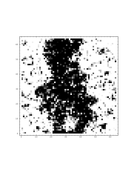
Figure 1: Interfaces in a typical mixed phase configuration for $\mu^{2}=1.40$ and $L=64$. Values of $\phi_{i}>0.5(<-0.5)$ have been depicted black (white), values of $|\phi_{i}|<0.5$ have been depicted by varying grey shades. For this configuration the magnetization was $m_{1}\approx-0.2$.

Figure 2: Flat multicanonical distributions as compared to the canonical double-peak histograms of $m_{1}$ after reweighting for $\mu^{2}=1.30$ and different lattice sizes $L=8,16$, and $32$.

Figure 3: Flat multicanonical distributions as compared to the canonical double-peak histograms of $m_{1}$ after reweighting for $L=64$ and $\mu^{2}=1.30,1.35$, and $1.40$. The arrow in Fig. 3c indicates the value of $m_{1}$ which was measured for the configuration displayed in Fig. 1.

Figure 4: Evolution series of $m_{1}$ for $L=16$ and $\mu^{2}=1.30$ using the canonical Metropolis (Fig. 4a), the multicanonical Metropolis (Fig. 4b), the canonical multigrid W-cycle (Fig. 4c), and the multicanonical multigrid W-cycle (Fig. 4d). In Figs. 4a and 4c we also show the digitalized time series according to the simple two-state flip model. The time scales were adjusted so that an evolution over roughly $30\tau^{\rm int}_{m_{1}}$ is displayed in each figure.

Figure 5: Autocorrelation time $\tau(k)$ together with a three-parameter fit according to eq. (16) for ${\cal O}=m_{1}\exp(f)$, $\mu^{2}=1.40$, $L=64$, and the multicanonical W-cycle. The horizontal line shows the integrated autocorrelation time $\tau^{\rm int}_{m_{1}e^{f}}=\tau(\infty)$ together with error bounds. The inset shows a logarithmic plot of the autocorrelation function $A(j)$ together with linear fits $\ln A(j)={\rm const}-j/\tau^{\rm exp}_{m_{1}e^{f}}$. See the text for a detailed explanation.

Figure 6: Effective autocorrelation times $\tau^{\rm eff}_{m_{1}}$ and integrated autocorrelation times $\tau^{\rm int}_{m_{1}e^{f}}$ as a function of $L$. Straight lines are fits according to $\tau=aL^{z}$.

Figure 7: Two-dimensional histograms of $m_{1}$ and $m_{2}$ simulated for $L=64$ and $\mu^{2}=1.40$ and reweighted to different values of $\mu^{2}$. The multicanonical distributions are shown in Fig. 7a for $\mu^{2}=1.40$ without reweighting, in Fig. 7c after reweighting to $\mu^{2}=1.375$, and in Fig. 7e after reweighting to $\mu^{2}=1.35$. Figs. 7b, 7d, and 7f show the respective canonical distributions after additional reweighting with the multicanonical reweighting factor $\exp(f(m))$.

Figure 8: Interface tension $\sigma_{L}$ as a function of $\mu^{2}$ for $L=8,16,32$, and $64$. The filled circles show the actual simulation data and the dashed lines were obtained by reweighting. The values for $\sigma=\sigma_{\infty}$ were obtained by an extrapolation according to $\sigma_{L}=\sigma_{\infty}+a/L$, and the solid straight line shows a fit $\sigma_{\infty}=a(\mu^{2}-\mu^{2}_{c})$ with $\mu^{2}_{c}=1.274(3)$.

References

- [1] J.D. Gunton, M.S. Miguel, and P.S. Sahni, in Phase Transitions and Critical Phenomena, Vol. 8, edited by C. Domb and J.L. Lebowitz (Academic Press, N.Y., 1983).
- [2] H.J. Herrmann, W. Janke, and F. Karsch (eds.), Dynamics of First Order Phase Transitions (World Scientific, Singapore, 1992).
- [3] B.A. Berg and T. Neuhaus, Phys. Lett. B267 (1991) 249; Phys. Rev. Lett. 68 (1992) 9.
- [4] W. Janke, B.A. Berg and M. Katoot, Nucl. Phys. B382 (1992) 649.
- [5] B.A. Berg, U. Hansmann, and T. Neuhaus, Phys. Rev. B47 (1993) 497; B.A. Berg, U. Hansmann, and T. Neuhaus, Z. Phys. B90 (1993) 229; U. Hansmann, B.A. Berg, and T. Neuhaus, in Ref.[2].
- [6] A. Billoire, T. Neuhaus, and B.A. Berg, Nucl. Phys. B396 (1993) 779; B413 (1994) 795.
- [7] B. Grossmann and M.L. Laursen, in Ref.[2]; and Nucl. Phys. B408 (1993) 637. B. Grossmann, M.L. Laursen, T. Trappenberg, and U.-J. Wiese, Phys. Lett. B293 (1992) 175.
- [8] B.A. Berg, in Ref.[2].
- [9] W. Janke, in Ref.[2].
- [10] C.F. Baillie, Int. J. Mod. Phys. C1 (1990) 91; R.H. Swendsen, J.-S. Wang, and A.M. Ferrenberg, New Monte Carlo Methods for Improved Efficiency of Computer Simulations in Statistical Mechanics, in The Monte Carlo Method in Condensed Matter Physics, edited by K. Binder (Springer, Berlin, 1992) p. 75; A.D. Sokal, Bosonic Algorithms, in Quantum Fields on the Computer, ed. M. Creutz (World Scientific, Singapore, 1992) p. 211; A.D. Kennedy, Nucl. Phys. B (Proc. Suppl.) 30 (1993) 96.
- [11] J. Goodman and A. D. Sokal, Phys. Rev. Lett. 56 (1986) 1015; Phys. Rev. D40 (1989) 2035.
- [12] G. Mack, in Nonperturbative quantum field theory, Cargèse 1987, ed. G.‘t Hooft et al. (Plenum, New York, 1988); G. Mack and S. Meyer, Nucl. Phys. B (Proc. Suppl.) 17 (1990) 293.
- [13] D. Kandel, E. Domany, D. Ron, A. Brandt, and E. Loh, Jr., Phys. Rev. Lett. 60 (1988) 1591; D. Kandel, E. Domany, and A. Brandt, Phys. Rev. B40 (1989) 330.
- [14] R.G. Edwards, J. Goodman, and A.D. Sokal, Nucl. Phys. B354 (1991) 289; A. Hulsebos, J. Smit, and J.C. Vink, Nucl. Phys. B356 (1991) 775; R.G. Edwards, S.J. Ferreira, J. Goodman, and A.D. Sokal, Nucl. Phys. B380 (1992) 621; M.L. Laursen and J.C. Vink, Nucl. Phys. B401 (1993) 745.
- [15] W. Janke and T. Sauer, Chem. Phys. Lett. 201 (1993) 499.
- [16] W. Janke and T. Sauer, in Path Integrals from meV to MeV, ed. H. Grabert et al. (World Scientific, Singapore, 1993) p. 17.
- [17] W. Janke and T. Sauer, Phys. Rev. E49 (1994) 3475.
- [18] K. Rummukainen, Nucl. Phys. B390 (1993) 621.
- [19] W. Kerler and A. Weber, Phys. Rev. B47 (1993) 11563.
- [20] A. Milchev, D.W. Heermann, and K. Binder, J. Stat. Phys. 44 (1986) 749.
- [21] R.C. Brower and P. Tamayo, Phys. Rev. Lett. 62 (1989) 1087.
- [22] R. Toral and A. Chakrabarti, Phys. Rev. B42 (1990) 2445.
- [23] B. Mehlig and B.M. Forrest, Z. Phys. 89 (1992) 89; B. Mehlig, A.L.C. Ferreira, and D.W. Heermann, Phys. Lett. B291 (1992) 151.
- [24] K. Binder, Z. Phys. B43 (1981) 119, Phys. Rev. A25 (1982) 1699.
- [25] N. Madras and A.D. Sokal, J. Stat. Phys. 50, 109 (1988).
- [26] G.M. Torrie and J.P. Valleau, Chem. Phys. Lett. 28 (1974) 578; J. Comp. Phys. 23 (1977) 187; I.S. Graham and J.P. Valleau, J. Phys. Chem. 94 (1990) 7894; J.P. Valleau, J. Comp. Phys. 96 (1991) 193.
- [27] W. Hackbusch, Multi-Grid Methods and Applications (Springer, Berlin, 1985).
- [28] S.F. McCormick (ed.), Multigrid Methods. Theory, Applications, and Supercomputing (Dekker, New York, 1988).
- [29] A.D. Sokal, New York University preprint NYU-TH-93/07/02.
- [30] T. Neuhaus, Nucl. Phys. B (Proc. Suppl.) 34 (1994) 667.
- [31] M. Grabenstein and K. Pinn, J. Stat. Phys. 71 (1993) 607.
- [32] R.G. Miller, Biometrika 61 (1974) 1; B. Efron, The Jackknife, the Bootstrap and other Resampling Plans (SIAM, Philadelphia, PA, 1982).
- [33] A. Billoire, R. Lacaze, A. Morel, S. Gupta, A. Irbäck and B. Peterson, Nucl. Phys. B358 (1991) 231; W. Janke, unpublished notes.
- [34] A.M. Ferrenberg and R.H. Swendsen, Phys. Rev. Lett. 61 (1988) 2635; ibid. 63 (1989) 1195; and Erratum, ibid. 63 (1989) 1658.
- [35] U.-J. Wiese, Bern preprint BUTP-92/37.