FSU-SCRI-94-123
AZPH-TH/94-26
IUHET-288
UUHEP-94/5

THERMAL PHASE TRANSITION IN MIXED ACTION SU(3) LATTICE GAUGE THEORY AND WILSON FERMION THERMODYNAMICS

T. Blum^a, C. DeTar^b, Urs M. Heller^c, Leo Kärkkäinen^a, K. Rummukainen^d, and D. Toussaint^a

^aDepartment of Physics, University of Arizona,
Tucson, AZ 85721, USA

^bDepartment of Physics, University of Utah,
Salt Lake City, UT 84112, USA

^cSCRI, The Florida State University,
Tallahassee, FL 32306-4052, USA

^dDepartment of Physics, Indiana University,
Bloomington, IN 47405, USA

Abstract

We study the thermal phase diagram of pure SU(3) lattice gauge theory with fundamental and adjoint couplings. We improve previous estimates of the position of the bulk transition line and determine the thermal deconfinement transition lines for $N_{t}=2,4,6,$ and 8. The endpoint of the bulk transition line $(\beta_{f},\beta_{a})=(4.00(7),2.06(8))$ improves upon earlier estimates obtained using smaller lattice sizes. For $N_{t}>4$ the deconfinement transition line splits cleanly away from the bulk transition line. With increasing $N_{t}$ the thermal deconfinement transition lines shift to increasingly weaker coupling, joining onto the bulk transition line at increasingly larger $\beta_{a}$ in a pattern consistent with the usual universality picture of lattice gauge theories. We also discuss the possible consequences of an induced adjoint term from the fermionic determinant and determine this induced term numerically with a microcanonical demon method for two flavors of dynamical Wilson fermions.

1 Introduction

The phase diagram of fundamental–adjoint pure gauge systems, shown in Fig. 1, is considerably more complicated than the one with only a fundamental coupling. Early studies found that it has first order (bulk) transitions in the region of small $\beta_{f}$ [1, 2]. For SU(3) the purely adjoint system has a transition at $\beta_{a}=6.5(3)$. For $\beta_{a}\to\infty$ the system reduces to a $Z_{3}$ gauge theory with a transition at $\beta_{f}=0.67$. In the $\beta_{a}$,$\beta_{f}$ plane these transition points are extended to lines that merge into a single terminating line segment as shown. As discussed in Sec. 3, we place the endpoint at $(\beta_{f},\beta_{a})=(4.00(7),2.06(8))$, considerably different from old results obtained on small lattices [2]. We also find a roughly straight line of bulk crossovers extending beyond the endpoint.

Figure 1: The phase diagram for the fundamental–adjoint system.

The non-trivial phase structure in the fundamental–adjoint plane, and in particular the critical endpoint of the transition line pointing toward the fundamental axis, has been shown to be associated with, or even responsible, for the dip in the discrete $\beta$-function of the theory with standard Wilson (fundamental) action, which occurs in the region where the bulk crossover line crosses the fundamental axis. The bulk transition might also mask the thermal deconfinement transition, at least for lattices with small temporal extent $N_{t}$. Indeed, from early simulations by Batrouni and Svetitsky [3] and by Gocksch and Okawa [4] we know that for pure gauge SU(4) theory, for which the bulk transition crosses the fundamental axis, the $N_{t}=2$ temperature transition joins the bulk line, but that for $N_{t}=4$ the bulk line and the thermal line exist separately.

In a recent paper Gavai, Grady and Mathur showed that at nonzero temperature the deconfinement transition in pure gauge SU(2) survives for positive adjoint couplings and is connected to the end point of the bulk transition line [5]. They were not able to distinguish the first order bulk line from the $N_{t}=4$ and 6 thermal transition lines in their simulations. Universality in the continuum limit requires that as $N_{t}$ is increased, the thermal phase transition line shifts to weaker coupling, so that approaching the zero-temperature weak-coupling limit along any line in the fundamental–adjoint coupling plane leads to the same low temperature, confined theory. Thus the thermal phase transition lines could not remain anchored to a bulk transition line for higher $N_{t}$. More recently Mathur and Gavai [6] raised doubts about the very existence of a bulk phase transition in SU(2), characterizing even the first-order portion of the line as a thermal deconfinement transition that is displaced toward weak coupling with increasing $N_{t}$. Clarification is obviously needed.

Puzzled by the finding of Ref. [5], but also motivated by some unexpected results in the study of the high temperature behavior of full QCD with Wilson fermions [7] that might be explained by the fact that the fermion determinant induces, among others, an effective adjoint coupling, we decided to study pure SU(3) gauge theory with a fundamental–adjoint action at finite temperature in more detail. We show that the first order bulk transition in pure gauge SU(3) in the fundamental–adjoint coupling plane indeed separates from the thermal deconfinement transition provided $N_{t}$ is made large enough.

According to universality arguments [8], QCD with only two massless quarks has a second order thermal deconfining phase transition, which becomes a smooth crossover if the quarks are massive. Lattice QCD simulations with two light flavors of staggered quarks support this scenario. However, with two flavors of Wilson quarks recent simulations indicate that at large values of the hopping parameter the phase diagram is more complicated [7]: for $N_{t}=6$ and at hopping parameter $\kappa\sim 0.19$ the system has a strong first order–like transition, where the plaquette expectation value has a sharp discontinuous jump. However, the average Polyakov loop remains small at this point, and starts to increase only when $\beta$ is considerably larger. This behavior is strongly reminiscent of separated bulk and thermal transitions, as in the pure gauge SU(3) model with mixed fundamental–adjoint action. In fact, these systems resemble each other so much that one is tempted to assume that the dynamical  reason for these transitions is the same: the dynamical Wilson fermions induce a strong adjoint term in the effective pure gauge action. We therefore set out to measure such an induced adjoint term employing a microcanonical demon method.

2 The fundamental–adjoint action

Let us consider the action $S$ for SU($N$) lattice gauge theory with fundamental and adjoint coupling:

$$S=\beta_{f}\sum_{P}[1-\frac{1}{N}{\rm Re}{\rm Tr}_{f}U_{P}]+\beta_{a}\sum_{P}[1-\frac{1}{N^{2}}{\rm Tr}_{f}U^{\dagger}_{P}{\rm Tr}_{f}U_{P}].$$ (1)

Here ${\rm Tr}_{f}={\rm Tr}$ is the trace in the fundamental representation, $U_{P}$ is the path ordered product of the link matrices along the elementary plaquette $P$. Using ${\rm Tr}_{a}U=|{\rm Tr}_{f}U|^{2}-1$ for the trace in the adjoint representation, the parametrization (1) is connected to the alternative one, used for general one-plaquette actions [9],

$$S=\beta_{f}\sum_{P}[1-\frac{1}{N}{\rm Re}{\rm Tr}_{f}U_{P}]+\beta_{a}^{\prime}\sum_{P}[1-\frac{1}{N^{2}-1}{\rm Tr}_{a}U_{P}]$$ (2)

by

$$\beta_{a}=\frac{N^{2}}{N^{2}-1}\beta_{a}^{\prime}.$$ (3)

The $\Lambda$-parameters of the standard Wilson and the fundamental–adjoint action are connected by [9]

$$\log\frac{\Lambda^{W}}{\Lambda^{FA}}=\frac{N^{2}+1}{8b_{0}}\left(\frac{\beta_{a}}{\beta_{f}+2\beta_{a}}\right)$$ (4)

with $b_{0}$ the one-loop coefficient of the $\beta$-function. Therefore, the equivalent Wilson coupling, in perturbation theory, is

$$\beta_{W}=\beta_{f}+2\beta_{a}-\frac{N^{2}+1}{2}\frac{\beta_{a}}{\beta_{f}+2\beta_{a}},$$ (5)

and lines of constant $\beta_{W}$ in (5) should represent lines of constant physics (up to two loop and non-perturbative corrections). Of course, at the relatively large couplings that we will be working with, the relation (5) is not very reliable. We shall try to improve the relation by using tadpole improved perturbation theory [10], where a factor $u_{0}$, with $u_{0}^{4}={\rm Tr}U_{P}/N$, is taken out of every link field $U_{\mu}$. In the relation (5) tadpole improvement amounts to the replacement $\beta_{a}\rightarrow u_{0}^{4}\beta_{a}$ with $u_{0}$ computed in the equivalent Wilson theory. Compensating for the $u_{0}^{4}$ as computed in perturbation theory then gives, instead

$$\beta_{W}=\beta_{f}+2\beta_{a}u_{0}^{4}-\frac{\beta_{a}u_{0}^{4}}{\beta_{f}+2\beta_{a}u_{0}^{4}}.$$ (6)

3 The phase diagram in the fundamental–adjoint coupling plane

Monte Carlo simulations with the mixed action described above were carried out using a standard Metropolis updating scheme. First we found it necessary to repeat the early calculation of Bhanot [2] to locate the endpoint of the bulk phase transition more accurately. This was done in a series of simulations with $8^{4}$ lattices by measuring the discontinuity in the average fundamental plaquette $E_{f}=\langle{\rm Tr}U_{P}\rangle$ and adjoint plaquette $E_{a}=\langle|{\rm Tr}U_{P}|^{2}/3\rangle$ along the first order line. Results are shown in Table 1. To support the identification as a bulk transition Fig. 2 shows $E_{f}$, obtained from various lattice sizes, as function of $\beta_{f}$ for $\beta_{a}=2.25$ We note that $E_{f}$ jumps for all lattices at the same point.

$\beta_{a}$	$\beta_{f}$	$\Delta E_{f}$	$\Delta E_{a}$
3.0	3.27	0.656( 2)	0.464(1)
2.75	3.47	0.547( 2)	0.398(2)
2.5	3.66	0.424( 5)	0.315(4)
2.35	3.77	0.336( 9)	0.250(7)
2.25	3.85	0.252(10)	0.193(8)

Table 1: The jumps in in the average plaquette and average adjoint plaquette values across the bulk transition line.

Figure 2: $E_{f}$ as function of $\beta_{f}$ for various lattice sizes, as indicated, at $\beta_{a}=2.25$.

The location of the phase transitions for the different values of $\beta_{a}$ considered was first obtained with runs from mixed starts. At the two $\beta_{f}$ values that straddle the transition we then made runs with hot and cold starts to obtain the gaps in Table 1. When we found metastable states in both cases we took the larger gap measured. In any case, the errors listed in Table 1 are statistical only. We estimate systematic errors to be of order 0.010 to 0.020 in $\Delta E_{f}$.

The endpoint of the bulk transition line $(\beta^{*}_{f},\beta^{*}_{a})$ is then estimated by fitting to

$$\Delta E_{f}=c~{}(\beta_{a}-\beta_{a}^{*})^{p}.$$ (7)

Such a fit works very well, as shown in Fig. 3, having $\chi^{2}=1.16$ for 2 degrees of freedom. In this region of the parameter space the bulk transition line is essentially straight, and from the endpoint value $\beta_{a}^{*}=2.06(8)$ we infer the location of the endpoint of the bulk transition line as

$$(\beta^{*}_{f},\beta^{*}_{a})=(4.00(7),2.06(8)),$$ (8)

shown with our improved location of the bulk phase transition line in Fig. 1. The error of 0.08 in $\beta_{a}^{*}$ includes our estimate of the systematic uncertainties in the gaps, resulting as mentioned above from not obtaining them exactly at the critical coupling. The statistical error from the fit to the data in Table 1 is only 0.03. The best fit values for the other parameters are $c=0.68(1)$ and $p=0.58(3)$.

Figure 3: The average plaquette gap $\Delta E_{f}$ as function of $\beta_{a}$ together with the fit to determine the endpoint $\beta_{a}^{*}$.

4 Results at nonzero temperature

As in pure SU(2), the SU(3) pure gauge deconfinement transition extends to non-zero $\beta_{a}$ values, since the global Z(3) symmetry is not affected by the addition of an adjoint coupling. As we increase the adjoint coupling the transitions for different $N_{t}$ move closer together, and closer to the so called crossover region from strong to weak coupling behavior, which can be regarded as an extension of the bulk phase transition line.

To explore the high temperature behavior of the mixed action theory, we studied the deconfinement transition on lattices with temporal extent $N_{t}=2$, 4, 6 and 8. Note that in the first 3 cases we limited ourselves to lattices with aspect ratio $N_{s}/N_{t}=2$. That proved sufficient to find the deconfinement transitions with sufficient accuracy. The thermal deconfinement transition point is defined as the location of maximum slope in the modulus of the Polyakov loop $\langle|P|\rangle$. All transition points we obtained are shown in Fig. 4 and Table 2. For $N_{t}=2$ the $\beta_{a}=0$ deconfinement transition continues smoothly into the bulk transition, which is shifted significantly from its large $N_{t}$ value, as $\beta_{a}$ increases. For $N_{t}=4$ at $\beta_{a}=2.0$ the deconfinement phase transition joins and is indistinguishable from from the bulk transition, just as was found for SU(2) [5]. But for $N_{t}=6$ at $\beta_{a}=2.0$, there is a clear separation, with the bulk crossover occurring at $\beta_{f}=4.035(5)$ and the thermal deconfinement transition at $\beta_{f}=4.07(2)$. At $\beta_{a}=2.25$, even for the $12^{3}\times 6$ lattice, bulk and deconfinement transition coincide, both occurring at $\beta_{f}=3.850(5)$.

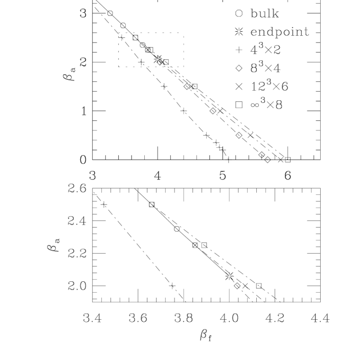
Figure 4: The phase diagram together with the thermal deconfinement transition points for $N_{t}=2$, 4, 6 and 8. The lower plot shows an enlargement of the region around the end point of the bulk transition.

$\beta_{a}$	$\beta_{f}$
	$N_{t}=2$	$N_{t}=4$	$N_{t}=6$	$N_{t}=8$
0.0	5.0941(4)	5.6925(2)	5.8941(5)	6.001(25)
0.5	4.75(5)	5.25(5)	5.425(20)	-
1.0	4.4(1)	4.85(5)	4.96(2)	-
1.5	4.1(1)	4.45(5)	4.525(20)	4.58(2)
2.0	3.75(5)	4.035(5)	4.07(2)	4.135(10)
2.25	-	3.845(5)	3.850(5)	3.89(1)
2.5	3.45(5)	-	-	3.660(5)

Table 2: The deconfinement transition points.

At larger $N_{t}$ the small size of the order parameter required additional care in locating the phase transition. We carried out a finite size analysis with simulations on $N_{s}^{3}\times 8$ lattices with $N_{s}=8$,12,16. In the confined phase $\langle|P|\rangle$ should vanish as $1/\sqrt{V_{s}}$ with increasing spatial volume, while in the deconfined phase it should extrapolate to a nonzero value. To treat both cases identical we made fits to $\langle|P|\rangle=P_{\infty}+c/\sqrt{V_{s}}$. The finite size analysis is shown for $\beta_{a}=2.25$ in Fig. 5. Plots for other $\beta_{a}$ are very similar. In this way we place the $N_{t}=8$ deconfinement transition for $\beta_{a}=2.0$ at $\beta_{f}=4.135(15)$, clearly separated from the bulk crossover as well as from the $N_{t}=6$ deconfinement transition. For $\beta_{a}=2.25$ the deconfinement transition occurs at $\beta_{f}=3.89(1)$, still separated from the bulk transition at $\beta_{f}=3.850(5)$, whereas at $\beta_{a}=2.50$, no clear separation is visible.

Figure 5: $\langle|P|\rangle$ at $\beta_{a}=2.25$ for $N_{t}=8$ and $N_{s}=8$, 12 and 16 and the extrapolation to $N_{s}=\infty$.

We conclude that with increasing $N_{t}$ the deconfinement transition line is displaced toward weaker coupling, joining onto the bulk transition at larger and larger values of $\beta_{a}$, consistent with universality. However, trying to see low temperature continuum physics at larger values of the adjoint coupling $\beta_{a}$ requires larger lattices to avoid strong violations of asymptotic scaling associated with the bulk transition line.

Having found non-perturbatively lines of constant physics, here defined as lines of the thermal deconfinement transition for fixed $N_{t}$, we can compare them to the perturbative predictions obtained from eq. (5). Not surprisingly, the perturbative prediction is poor. Using, instead, the tadpole improved prediction eq. (6) changes the perturbative result in the right direction, but still fails to give the correct lines of constant physics, as shown in Fig. 6. It is interesting to notice, though, that $E_{f}=\langle{\rm Tr}U_{P}\rangle$ is almost constant along the deconfinement transition lines. Therefore, equal effective coupling $\beta_{\rm eff}=2/(1-E_{f}/3)$ describes lines of constant physics remarkably well.

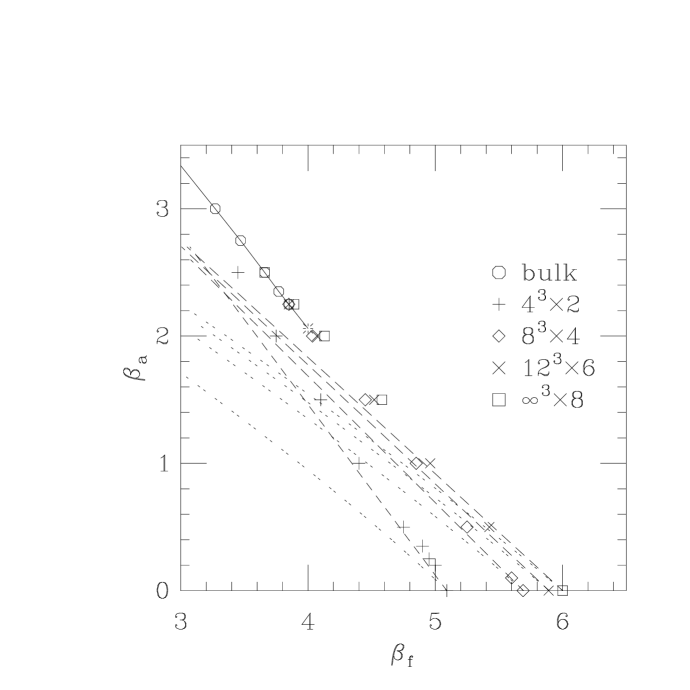
Figure 6: Lines of constant physics as predicted by perturbation theory (dotted lines) and tadpole improved perturbation theory (dashed lines) together with the deconfinement transitions for $N_{t}=2$, 4, 6, and 8.

5 Couplings induced by the fermionic determinant

Full QCD simulations with two flavors of staggered fermions support the view that there is no thermal phase transition at positive quark masses, and a second order transition at zero quark mass [11] (a scenario also supported by universality arguments [8]). However, the phase diagram with dynamical Wilson fermion has turned out to be complicated for large values of the hopping parameter. It was found that for $N_{t}=6$ and hopping parameter $\kappa\sim 0.19$, there is an apparent first order transition leading to a jump in the average plaquette. At slightly higher $\beta_{f}$ the Polyakov loop expectation value $\langle{\rm Re}P\rangle$ remains small in a manner remarkably similar to our findings for the region separating the bulk and thermal phase transition in the mixed action pure gauge theory. It is tempting to speculate that the first order phase transition seen with Wilson quarks is a bulk transition related to the first order pure gauge adjoint bulk transition.

It has been shown, that the location of the deconfinement transition with staggered fermions can be surprisingly well explained by a change in the fundamental coupling induced by heavy fermions [12]. Let us see how new terms in the gauge action are induced by Wilson fermions. The discretized action $S_{0}$ for $n_{f}$ flavors of Wilson fermions is

$$S_{0}=S_{g}+\sum_{f=1}^{n_{f}}\sum_{n,m}{\bar{\psi}}_{n}^{f}M_{nm}[U]\psi_{m}^{f},$$ (9)

where

$$M_{nm}[U]=\delta_{nm}-\kappa\sum_{\mu}((1-\gamma_{\mu})U_{n\mu}\delta_{n+\mu,m}+(1+\gamma_{\mu})U^{\dagger}_{n\mu}\delta_{n-\mu,m})$$ (10)

and $S_{g}$ is the pure gauge action. The fermions can be integrated out and the effective gauge action $S_{\rm eff}$ can be obtained by a hopping parameter ($\kappa$) expansion.

$$S_{\rm eff} =S_{g}-n_{f}{\rm Tr}\ln M[U]$$ (12)

$$=S_{g}+n_{f}\sum_{C}\kappa^{l[C]}{\frac{1}{l[C]}}{\rm Tr}\left(\prod_{C}(1\pm\gamma_{\mu})\right)\cdot\left({\rm Tr}U_{C}+{\rm Tr}U^{\dagger}_{C}\right),$$

where the sum is over all (unoriented) closed loops $C$ and $l[C]$ is the length of the loop. For small hopping parameters $\kappa$, the shift for the fundamental coupling comes from loops around a single plaquette and is given by $\Delta\beta_{f}=n_{f}{\frac{4}{3}}\kappa^{4}$. The shift in the adjoint coupling comes from closed loops winding three times around a plaquette. For small $\kappa$ it is $\Delta\beta_{a}\propto\kappa^{12}$. Similarly the staggered fermion action induces an adjoint coupling. Indeed with eight flavors, a bulk transition has been found [13], but studies have not yet been done to determine whether there is evidence for a similar separation of the bulk transition and the thermal crossover.

The hopping parameter expansion outlined above is accurate only when $\kappa$ is very small. Results with much broader validity range can be obtained with the heavy quark perturbation method. This method was used by Hasenfratz and DeGrand [12] to calculate $\Delta\beta_{f}$. They found shifts $\Delta\beta_{f}$ that agreed very well with MC data. However, such a heavy quark perturbation calculation has not been performed for $\Delta\beta_{a}$.

5.1 Demon Algorithm

We use the microcanonical demon method [14, 15, 16] to project out the induced effective gauge action from full fermionic simulations. Our ansatz for the effective action is given by eq.  (1), with a priori unknown coupling constants $\beta_{i}=\beta_{f}$ or $\beta_{a}$. For both of the coupling constants we introduce a demon , which is a real-valued action variable with $0\leq D_{i}\leq D_{i}^{\rm max}$. Effectively, the fermionic action is used as a heat bath to thermalize the demons: starting from a configuration generated with the original action, we update the system microcanonically with demons. During the microcanonical update $S_{i}+D_{i}={\rm const.}$ separately for both fundamental and adjoint parts of the action. After the microcanonical update, the old gauge configuration is discarded, and the demon update is started again from a new gauge configuration, while preserving the demon values. The principle of the method is shown graphically in fig. 7.

Figure 7: Flow diagram of the demon algorithm. The configurations are generated with the original fermionic action $S_{0}$ (top) eq. (9), and copied for the microcanonical demon update. At the end of the microcanonical update, the demon values are copied for the next update phase (bottom).

The microcanonical update phase is performed with a Metropolis algorithm: the proposed new gauge link is accepted only if the demons can give or take the amount of energy needed:

$$\Delta S_{i}\geq D_{i}{\hskip 14.22636pt}\mbox{and}{\hskip 14.22636pt}-\Delta S_{i}\leq D_{i}^{\rm max}-D_{i}$$ (13)

for both $i=f$ or $a$. Because both of the demons have to accept the update step for it to be performed, the demon distributions are correlated. After the whole update procedure is repeated many times, the demons attain an equilibrium distribution and we can measure $\langle D_{i}\rangle$. The induced effective couplings can be solved from equations

$$\langle D_{i}\rangle=\frac{1}{\beta_{i}}-\frac{D_{i}^{\rm max}}{\exp(\beta_{i}D_{i}^{\rm max})-1}\,.$$ (14)

It is not necessary to limit the demon action from above if the expected value of the corresponding coupling constant is large. In our case, we had to limit only the adjoint demon values from above; for the fundamental demon $D_{f}^{\rm max}=\infty$ and in this case eq. (14) reduces to $\beta_{f}=1/\langle D_{f}\rangle$.

One drawback of the demon method is that the final results can depend on the details of the update procedure. Some of the factors affecting the results are the range and shape of the distribution from which the new gauge matrix is chosen in the Metropolis update (true even if the detailed balance is always satisfied), the acceptance rate, and the ‘length’ of the demon update phase: one can update each configuration microcanonically until the demons and the systems are properly thermalized, or one can stop the update after only one – or even partial – update sweep. These effects are easy to observe in some simple test models where the energy distributions can be exactly calculated. This does not mean that some methods are correct, some incorrect; different methods only correspond to different projections from the original action to the functional space spanned by the ansatz for the effective action. Nevertheless, one should not ignore this problem when using the demon method. Furthermore, let us note that if the effective action is completely equivalent to the original action, the above effects vanish and the demon method yields a unique $\beta_{i}$. Conversely, if the effective action is close to the true action – which should be the case for all reasonable effective actions – one can expect that the differences between the methods will be small.

The autocorrelations between configurations can introduce further systematic errors [16]. These errors are unrelated to the errors above. However, in most cases the differences are expected to behave as $1/V$ as $V\rightarrow\infty$ (the heat capacity of the system $\gg$ the heat capacity of the demons).

In our case we have a dramatically truncated effective action, and a priori we do not have any guarantee of the ‘goodness’ of the ansatz. The results were checked by using different update schemes: we performed 1 or 20 trajectories with the fermionic action between the microcanonical update phases, and 1/8, 1 or 50 microcanonical update sweeps for each gauge configuration. In all our tests the possible differences were completely overwhelmed by the statistical noise, indicating that the method is quite robust to the accuracy we reached. The results given below are all calculated by performing one microcanonical update sweep for each gauge configuration and after each fermionic trajectory.

5.2 Simulations and Results

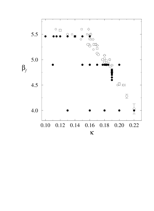
Figure 8: The location of the dynamical Wilson fermion runs in the $(\beta^{0}_{f},\kappa)$-plane (filled circles). The open circles indicate the location of the $N_{t}=4$ finite temperature crossover, the squares the $N_{t}=6$ phase transition, and the diamonds the zero-temperature $\kappa_{c}$. The data is from ref. [7] and from references therein.

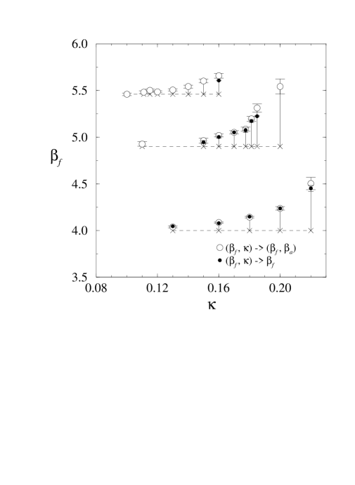
Figure 9: The induced $\beta_{f}$. Small crosses on horizontal dashed lines indicate the simulation $(\beta_{f}^{0},\kappa)$, open circles and black dots the measured $\beta_{f}$-values using the effective fundamental–adjoint and fundamental only gauge action, respectively. The length of the vertical bars gives the magnitude of the induced $\Delta\beta_{f}$.

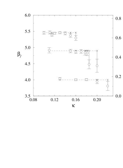
Figure 10: The induced $\beta_{a}$. The scale on the right gives the magnitude of the induced $\beta_{a}$, measured as the vertical distance between the plot symbols and dashed horizontal lines. Points below the dashed lines indicate negative $\beta_{a}$.

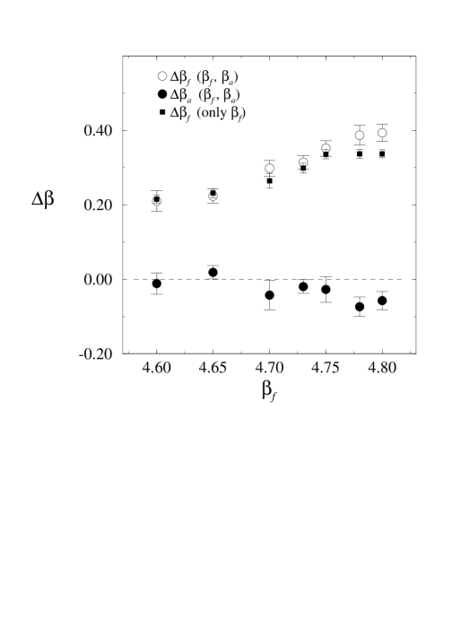
Figure 11: The induced $\beta_{f}$ and $\beta_{a}$, when $\kappa=0.19$.

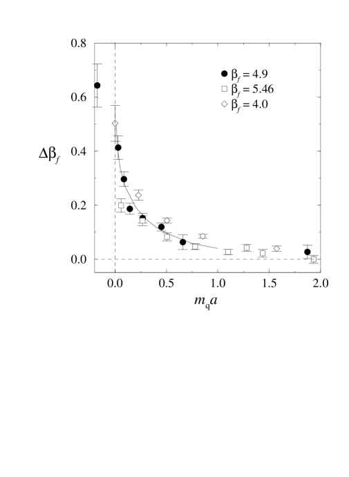
Figure 12: Comparison of the analytical result for $\Delta\beta_{f}$ [12] by Hasenfratz and DeGrand (solid line) to the MC data.

We tested the demon method by applying it to pure gauge fundamental–adjoint simulations. On a $4^{4}$-lattice we simulated the system at couplings $(\beta_{f},\beta_{a})_{0}=(3.6,1.8)$ and $(4.0,2.0)$. The induced couplings were $(3.594(6),1.812(17))$ and $(4.017(27),1.92(6))$, respectively, compatible with the input values. The latter coupling pair is very close to the bulk transition line in the $(\beta_{f},\beta_{a})$-plane. When we used an effective action consisting only of the $S_{f}$-part, $\beta_{f}$ was 4.688(9) and 6.044(12); the latter value is very close to the extension of the bulk transition line to the $\beta_{a}=0$ -axis.

If the Wilson fermion action induces a strong adjoint coupling giving rise to a bulk fundamental–adjoint transition, one should be able to observe the induced coupling already in small volumes. We performed simulations on $4^{4}$ lattices with 28 different $(\beta^{0}_{f},\kappa)$ pairs. Fig. 8 shows the location of all runs performed. In Figs. 9 and 10 we show the measured $\beta_{f}$ and $\beta_{a}$ calculated with $\beta^{0}_{f}=4.0$, 4.9, 5.46, and several $\kappa$ values, and in Fig. 11 the results with constant $\kappa=0.19$. In Figs. 9 and 11 we also show $\beta_{f}$ when $S_{\rm eff}=\beta_{f}S_{f}$ only.

When $\kappa$ is small, the quarks are very massive and the induced couplings are quite small (left side of Figs. 9 and 10). When $\kappa$ is increased, we approach the critical line where $m_{\rm q}\rightarrow 0$, and the fermionic contribution to the action becomes more significant. This is clearly visible as an increase in $\beta_{f}$ in Figs. 9 and 11. The critical values of $\kappa$ are approximately 0.16 ($\beta^{0}_{f}=5.46$), 0.19 (4.9) and 0.22 (4.0). We observe no significant increase in $\beta_{a}$; on the contrary, when $\kappa_{c}$ is approached, the induced $\beta_{a}$ becomes slightly negative! The minor role of the adjoint action is also evident from the fact that $\beta_{f}$ remains practically the same whether we use the $S_{a}$-term of the effective action or not. We also checked the results with a few simulations on $6^{4}$ lattices with similar results.

In Fig. 12 we compare $\Delta\beta_{f}$ to the predictions of ref. [12], as a function of quark mass $m_{\rm q}a=\kappa^{-1}-\kappa_{c}^{-1}$. The agreement is very good, especially when $\beta_{f}^{0}=4.9$.

6 Conclusions

We have shown that the fundamental–adjoint pure SU(3) gauge theory behaves as expected near the first order bulk transition. The thermal deconfinement transition lines join onto the bulk transition lines for larger and larger $\beta_{a}$. For $N_{t}=2$ the thermal transition continues smoothly into the bulk transition which is, however, shifted from its location for larger $N_{t}$. The $N_{t}=4$ thermal transition line joins the bulk transition line very close to the end point at $\beta_{a}\sim 2.0$, for $N_{t}=6$ at $\beta_{a}\sim 2.25$ and for $N_{t}=8$ at $\beta_{a}\sim 2.5$. Before joining the bulk transition line, the thermal transition line for a larger $N_{t}$ is to the right (at larger $\beta_{f}$) than for a smaller $N_{t}$. This finding is in agreement with what is expected from the usual universality picture of lattice gauge theories.

We speculated that the bulk transition observed with Wilson fermions for $N_{t}=6$ and large $\kappa$ [7], that looked very reminiscent of the situation seen in the pure gauge fundamental–adjoint action model, might be caused by an induced adjoint coupling. However, in measurements with the microcanonical demon method we did not observe that Wilson fermions induce any significant adjoint term in the pure gauge effective action, while the induced fundamental term is very well described by analytical calculations. It is thus very improbable that the transition observed in $N_{t}=6$ Wilson thermodynamics simulations could be explained by the fundamental–adjoint pure gauge transition, and the real cause of this phenomenon remains to be uncovered.

Acknowledgments

This work was partly supported by the U. S. Dept. of Energy under grants # DE-FG02-8SER40213, # DE-FG05-85ER250000, # DE-FG05-92ER40742, and # DE-FG02-91ER40661, and the U.S. National Science Foundation under grants PHY9309458. LK wants to thank the Antti Wihuri foundation for additional support. TB, CD, LK, KR and DT thank the Institute for Theoretical Physics, Santa Barbara, where the dynamical Wilson fermion part of this project was initiated. KR would like to thank M. Hasenbusch for many useful discussions. Computations were carried out on the UNIX clusters at the Supercomputer Computations Research Institute at The Florida State University and at the Pittsburgh Supercomputer Center, using several workstations in parallel with PVM, on IBM RS6000 workstations at the University of Utah and Indiana University, and on SUN workstations at the University of Arizona and Indiana University. Many of the simulations on the larger lattices were done on the IBM SP1 at the Cornell Theory Center, which receives major funding from the U.S. National Science Foundation and the State of New York, with additional funding from the Advanced Research Projects Agency, the National Institute of Health, IBM Corporation, and other members of the Cornell Theory Center’s Corporate Research Institute.

References

- [1] J. Greensite and B. Lautrup, Phys. Rev. Lett. 47 (1981), 9.
- [2] G. Bhanot, Phys. Lett. 108B (1982) 337.
- [3] G. G. Batrouni and B. Svetitsky, Phys. Rev. Lett. 52 (1984) 2205.
- [4] A. Gocksch and M. Okawa, Phys. Rev. Lett. 52 (1984) 1751.
- [5] R.V. Gavai, M. Grady, M. Mathur, Nucl. Phys. B423 (1994) 123.
- [6] Manu Mathur and R. V. Gavai, Universality and the Deconfinement Phase Transition in SU(2) Lattice Gauge Theory, preprint BI-TP 94/52, TIFR/TH/94-31, hep-lat/9410004.
- [7] T. Blum, T.A. DeGrand, C. DeTar, S. Gottlieb, A. Hasenfratz, L. Kärkkäinen, D. Toussaint and R.L. Sugar, Phys. Rev. D50 (1994) 3377.
- [8] R. Pisarski and F. Wilczek, Phys. Rev. D29 (1984) 338; F. Wilczek, J. Mod. Phys. A7 (1992) 3911.
- [9] A. Gonzales-Arroyo and C. P. Korthals-Altes, Nucl. Phys. B220 [FS8] (1982) 46.
- [10] G.P. Lepage and P. Mackenzie, Phys. Rev. D48 (1993) 2250.
- [11] F. Karsch, Phys. Rev. D49 (1994) 3791.
- [12] A. Hasenfratz, T. DeGrand, Phys. Rev. D49 (1994) 466.
- [13] F.R. Brown, H. Chen, N.H. Christ, Z. Dong, R. Mawhinney, W. Schaffer and A. Vaccarino, Phys. Rev. D46 (1992) 5655.
- [14] M. Creutz, A. Gocksch, M. Ogilvie, M. Okawa, Phys. Rev. Lett. 53 (1984) 875.
- [15] K. Yee, LSU-0725-94; hep-ph/9407383.
- [16] M. Hasenbusch, K. Pinn, C. Wieczerkowski, CERN-TH-7730/94; hep-lat/9411043.