String tension and monopoles in $T\neq 0$ SU(2) QCD

Abstract

Monopole and photon contributions to abelian Wilson loops are calculated using Monte-Carlo simulations of finite-temperature $SU(2)$ QCD in the maximally abelian gauge. The string tension is reproduced by monopole contribution alone also in finite temperature SU(2) QCD. The spatial string tension scales as $\sqrt{\sigma}\propto g^{2}(T)T$ and is reproduced almost by monopole contribution alone. Each configuration has one long monopole loop, and the long monopole loops alone are responsible for the string tension in the confinement phase. On the other hand, the spatial string tension in the deconfinement phase is reproduced by wrapped monopole loops alone.

1 Introduction

The dual Meissner effect due to condensation of color magnetic monopoles is conjectured to be the color confinement mechanism in QCD. We consider QCD after abelian projection[1]. The abelian projection of QCD is to extract an abelian theory performing a partial gauge-fixing.

A gauge called maximally abelian (MA) gauge is interesting among many abelian projections[2]. The string tension can be reproduced from residual abelian link variables[3]. Moreover, the string tension is explained by monopole contributions alone[4] as in compact QED [5].

The aim of this note is 1) to show that the string tension is explained by monopole contribution alone also in finite-temperature $SU(2)$ QCD, 2) to study the spatial string tension both in the confinement and in the deconfinement phases and 3) to study what kind of monopole loops are responsible for the physical and the spatial string tensions.

2 Formalism and simulations

We adopt the usual $SU(2)$ Wilson action and choose the maximally abelian gauge in which diagonal components of all link variables are maximized. Gauge fixed link variables are decomposed into a product of two matrices: $\widetilde{U}(s,\hat{\mu})=c(s,\mu)u(s,\mu)$ where $u(s,\mu)$ is diagonal abelian gauge field. An abelian Wilson loop operator is given by a product of monopole and photon contributions[4].

$$W\ = W_{1}\cdot W_{2}$$ (1)

$$W_{1} = \exp\{-i\sum\partial^{\prime}_{\mu}\bar{f}_{\mu\nu}(s)D(s-s^{\prime})J_{\nu}(s^{\prime})\}$$

$$W_{2} = \exp\{2\pi i\!\sum\!k_{\beta}(s)D(s\!-\!s^{\prime}\!)\frac{1}{2}\epsilon_{\alpha\beta\rho\sigma}\partial_{\alpha}M_{\rho\sigma}(\!s^{\prime}\!)\},$$

where $\partial$ $(\partial^{\prime})$ is a forward (backward) derivative on the lattice, $J_{\mu}(s)$ is an external current taking $\pm 1$ along the Wilson loop and $M_{\mu\nu}(s)$ is an antisymmetric variable as $J_{\nu}(s)=\partial_{\mu}^{\prime}M_{\mu\nu}(s)$ also $f_{\mu\nu}(s)=\bar{f}_{\mu\nu}(s)+2\pi n_{\mu\nu}=\partial_{\mu}\theta_{\nu}(s)-\partial_{\nu}\theta_{\mu}(s)$ $(-\pi<\bar{f}_{\mu\nu}(s)\leq\pi)$, where $\theta_{\mu}(s)$ is the angle variable defined from $u(s,\hat{\mu})$. $D(s)$ is the lattice Coulomb propagator and a monopole current $k_{\mu}(s)$ is defined as $k_{\mu}(s)=(1/4\pi)\epsilon_{\mu\alpha\beta\gamma}\partial_{\alpha}\bar{f}_{\beta\gamma}(s)$ following DeGrand-Toussaint[6]. $W_{1}(W_{2})$ is the photon (the monopole) contribution to the abelian Wilson loop. To study the features of both contributions, we calculated the expectation values of $W$ (called abelian), of $W_{1}$ (photon part) and of $W_{2}$ (monopole part), separately.

The Monte-Carlo simulations were performed on $24^{3}\times 8$ lattice at $\beta=2.3\sim 2.8$. All measurements were done every 50 sweeps after a thermalization of 2000 sweeps. We took 50 configurations totally for measurements. Assuming the static potential is given by linear + Coulomb + constant terms, we tried to determine the potential by the Creutz ratios using the least square fit.

The data are shown in Fig. 1. We calculated the physical string tension and the spatial string tension. The latter is given by Wilson loops composed of only spatial link variables. In the confinement phase, both string tensions from the abelian Wilson loops show the same value as that in ($T=0$) $SU(2)$ QCD, which is also the same as the full string tension[4]. Moreover, the physical string tension vanishes at the critical coupling $\beta_{c}$. However, the spatial string tension does not vanish and remains finite even in the deconfinement phase. Both physical and spatial string tensions from the monopoles almost agree with those from the abelian Wilson loops in the confinement phase. In the deconfinement phase, the monopole contributions to the physical string tension vanish, whereas those to the spatial one remain non-vanishing. The string tension from the photons is negligibly small.

Figure 1: Physical string tensions (circle) and spatial string tensions (square) from the abelian Wilson loops (upper) and from the monopoles (lower). The triangles are physical string tensions from the photons.

3 Scaling properties of the spatial string tension for $T>T_{c}$

It is believed that, at high temperature, four dimensional QCD can be regarded through dimensional reduction as an effective three dimensional QCD with $A^{0}$ as a Higgs field[8]. In this effective theory, the spatial string tension is expected to obey $\sqrt{\sigma_{s}(T)}\propto g^{2}(T)T,$ where $g(T)$ is the four dimensional coupling constant. The scaling properties of the spatial string tension derived from the usual full Wilson loops is confirmed recently in Monte-Carlo simulations of $SU(2)$ QCD[9].

To check if the same thing happens in the abelian case, we performed additional Monte-Carlo simulations varying both $N_{t}$ and $\beta$ on $24^{3}\times N_{t}$ lattices following Bali et al.[9]. We measured the string tension for $N_{t}=2,4,6,8\ {\rm and}\ 12$ at $\beta=2.30,2.51\ {\rm and}\ 2.74$ which are the critical points for $N_{t}=4,8\ {\rm and}\ 16$, respectively.

The data are plotted in Fig. 2. In the case of the spatial string tension derived from the abelian Wilson loops, we get almost the same behaviors as those of the full ones denoted by cross points. The latter is cited from Ref.[9]. $\sqrt{\sigma}/T_{c}$ is independent of $\beta$ and so the spatial string tension is expected to be a physical quantity remaining in the continuum limit. The spatial string tension from the monopoles is also $\beta$ independent, and is a little bit lower, but shows almost the same behavior.

Figure 2: The spatial string tensions from the abelian Wilson loops (upper) and from the monopoles (lower) versus temperature. The crosses denote full spatial string tensions.

4 A long monopole loop, a wrapped monopole loop and the string tension

The features of the abelian monopole currents were studied in [7] through Monte-Carlo simulations. They obtained the followings: 1) In the confinement phase, there is one long monopole loop in each configuration. 2) In the deconfinement phase, long monopole loops disappear. All monopole loops are short.

These results bring us an idea that the long monopole current plays an important role in the string tension, because the physical string tension exists only in the confinement phase and vanishes in the deconfinement phase. We investigated contributions from the longest monopole loops and from all other monopole loops to the string tension separately. The data on $24^{3}\times 8$ lattice are shown in Fig. 3. Clearly, the contributions from the long loop alone reproduce almost the full value of the string tension. On the other hand, the short loop contributions are almost zero. Only a few percent of the total links are occupied by monopole currents belonging to the long loop. Nevertheless, it gives rise to the full value of the string tension.

Next, we consider the case of the spatial string tension at high temperature. The static (wrapped) monopole , which closes by periodicity of the time direction, is expected to be important for the spatial string tension, because, in three dimensional SU(2) QCD with a Higgs field, the confinement mechanism is explained by an instanton [10], and this instanton is a static monopole in terms of four dimensional QCD at high temperature. We calculated the contributions from the wrapped loops and the non-wrapped loops to the string tension separately. The data on $16^{3}\times 4$ lattice are plotted in the Fig. 4. About $30\%$ of the monopole currents are the wrapped monopole currents in deconfinement phase. The contributions from the wrapped loop alone reproduce almost the full value of the spatial string tension from the total monopoles, whereas those from the non-wrapped loops are almost zero.

Details are published in [11]. This work is financially supported by JSPS Grant-in Aid for Scientific Research (B)(No.06452028).

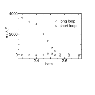
Figure 3: The contributions from the longest monopole loop (circle) and from all other monopole loops (square) to the string tensions.

Figure 4: The contributions from the wrapped loops (square), from the non-wrapped loops (diamond) and from the total monopole loops (circle) to the spatial string tensions.

References

- [1] G. ’tHooft, Nucl. Phys. B190, (1981) 455.
- [2] A.S. Kronfeld et al., Phys. Lett. B198, (1987) 516; A.S. Kronfeld et al., Nucl.Phys. B293, (1987) 461.
- [3] T. Suzuki and I. Yotsuyanagi, Phys. Rev. D42, (1990) 4257.
- [4] H.Shiba and T.Suzuki, Phys. Lett. B333, (1994) 461.
- [5] J.D. Stack and R.J. Wensley, Nucl. Phys. B371, (1992) 597.
- [6] T.A. DeGrand and D. Toussaint, Phys. Rev. D22, (1980) 2478.
- [7] S.Kitahara et al., in preparation.
- [8] T.Appelquist and R.D.Pisarski, Phys. Rev. D23, (1981) 2305.
- [9] G.S.Bali et al., Phys. Rev. Lett. 71, (1993) 3059.
- [10] Polyakov, Nucl. Phys. B120, (1977) 429.
- [11] Ejiri et al., to appear in Phys. Lett. B.