Structure of flux tube in $SU(2)$ lattice gauge theory

Abstract

The structure of the flux tube is studied in $SU(2)$ QCD from the standpoint of the abelian projection theory. It is shown that the flux distributions of the orthogonal electric field and the magnetic field are produced by the effect that the abelian monopoles in the maximally abelian (MA) gauge are expelled from the string region.

1 Introduction

It is important to investigate the structure of the flux tube in order to understand the confinement mechanism. A possible mechanism is the dual Meissner effect due to the condensation of the abelian monopoles, which is the basic idea of the abelian projection theory[1]. From the standpoint of this theory, the flux distribution in the flux tube is explained by the following two effects:

1. The effect that the abelian monopoles are expelled from the string region.

2. The squeezing of the abelian electric flux into the string region.

The purpose of this work is to check the validity of this picture (in the MA gauge).

2 Color distribution around a monopole

If monopoles have no correlation with color fields, they can not contribute directly to the color distribution in the flux tube. In order to investigate the color distribution around a monopole, we introduce a correlation function

$$p^{mon}_{\mu\nu}({\bf r})=\frac{\langle\delta^{mon}(c({\bf x},x_{0}))P_{\mu\nu}({\bf x}+{\bf r},x_{0})\rangle}{\langle\delta^{mon}\rangle}-\langle P_{\mu\nu}\rangle,$$

with $P_{\mu\nu}(x)=1-\frac{1}{2}tr[U_{\mu}(x)U_{\nu}(x+\hat{\mu})U^{\dagger}_{\mu}(x+\hat{\nu})U^{\dagger}_{\nu}(x)]$ being the plaquette action. $c({\bf x},x_{0})$ is a spatial cube located at $({\bf x},x_{0})$ and $\delta^{mon}(c)$ is an operator defined by

$$\delta^{mon}(c)=\left\{\begin{array}[]{ll}1&\mbox{if $c$ contains a monopole,}\\ 0&\mbox{otherwise.}\end{array}\right.$$

$p^{mon}_{\mu\nu}({\bf r})$ measures the difference between the average of the plaquette action in the presence of a monopole, separated by ${\bf r}$, and its vacuum expectation. We performed Monte Carlo simulations on a $16^{4}$ lattice at $\beta=2.5$. The Degrand-Toussaint scheme was used for determining the magnetic charge in a cube from abelian gauge fields after the abelian projection in the MA gauge[2].

In Fig.1, $p^{mon}_{\mu\nu}$ is plotted against $R$, the distance from the center of the cube to the plaquette. Monopoles correlate to color fields around themselves: the average of the plaquette action is large in the vicinity of a monopole and decreases to the vacuum expectation as the distance becomes large $(R>2)$.

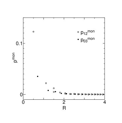
Figure 1: The correlation $p^{mon}_{\mu\nu}$ versus $R$.

3 Monopole contribution to the flux tube

The flux distribution in the presence of a static $q\bar{q}$ pair is measured by the correlation function:

$$p_{\mu\nu}({\bf x})=\frac{\langle W(R,T)\ P_{\mu\nu}({\bf x},T/2)\rangle}{\langle W(R,T)\rangle}-\langle P_{\mu\nu}\rangle,$$

where $W(R,T)$ is a Wilson loop of the size $R\times T$. Position of the plaquette relative to the $q\bar{q}$ sources is specified by ${\bf x}$. The squared electric and magnetic field components (in Minkowski space) relative to the vacuum are given by

$$(E^{2}_{1},E^{2}_{2},E^{2}_{3})=-2\frac{\beta}{a^{4}}(p_{01},p_{02},p_{03}),$$

$$(B^{2}_{1},B^{2}_{2},B^{2}_{3})=2\frac{\beta}{a^{4}}(p_{23},p_{31},p_{12}).$$

From these fields, the energy and action densities are obtained:

$${\cal E}=\frac{1}{2}[{\bf E}^{2}+{\bf B}^{2}],\ {\cal S}=\frac{1}{2}[{\bf E}^{2}-{\bf B}^{2}].$$

An interesting feature of the flux distribution measured is that the magnetic energy density relative to the vacuum is negative in contrast to the positive electric energy density. From the standpoint of the abelian projection theory, it is expected that this feature can be explained by abelian monopoles. The monopoles, which possibly correspond to Cooper Pairs in a superconductor, may be expelled from the string region of the flux tube. This indicates that the monopole density is lower in the inner part of the flux tube than in the vacuum. Such a behavior is also observed on the lattice, in the MA gauge[3]. In addition, the average of the plaquette action is large in the vicinity of a monopole, as shown in the previous section. As a result, the monopoles can make negative contributions to the correlation $p_{\mu\nu}({\bf x})$ in the string region. This means that the monopole contributions are positive for the electric energy density and are negative for the magnetic energy density.

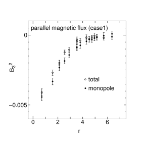
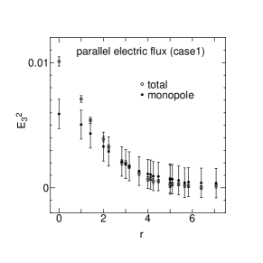
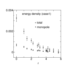
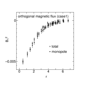
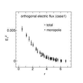
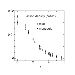
Figure 2: Flux distributions and monopole contributions. $r$ is the transverse distance from the $q\bar{q}$ axis.

To determine the monopole contributions quantitatively, we separate the whole lattice into the core regions corresponding to the monopole cores and the interstitial regions between them on the basis of the observation in the previous section. We define operators $\delta^{I}_{\mu\nu}(x)$ and $\delta^{II}_{\mu\nu}(x)$ on a plaquette by

$$\delta^{I}_{\mu\nu}(x)=\left\{\begin{array}[]{ll}1&\mbox{if plaquette $(x;\mu,\nu)$ belongs to}\\ &\mbox{the core regions,}\\ 0&\mbox{otherwise,}\end{array}\right.$$

$$\delta^{II}_{\mu\nu}(x)=1-\delta^{I}_{\mu\nu}(x).$$

The correlation $p_{\mu\nu}({\bf x})$ can be decomposed into $p_{\mu\nu}({\bf x})=p^{M}_{\mu\nu}({\bf x})+p^{F}_{\mu\nu}({\bf x})$, where

$$p^{M}_{\mu\nu}({\bf x})=\sum_{i}[\langle\delta^{i}_{\mu\nu}({\bf x})\rangle_{q\bar{q}}-\langle\delta^{i}_{\mu\nu}\rangle]\langle P^{i}_{\mu\nu}\rangle_{vac},$$

$$p^{F}_{\mu\nu}({\bf x})=\sum_{i}\langle\delta^{i}_{\mu\nu}({\bf x})\rangle_{q\bar{q}}[\langle P^{i}_{\mu\nu}({\bf x})\rangle_{q\bar{q}}-\langle P^{i}_{\mu\nu}\rangle_{vac}],$$

$$\langle\delta^{i}_{\mu\nu}({\bf x})\rangle_{q\bar{q}}=\frac{\langle W(R,T)\delta^{i}_{\mu\nu}({\bf x},T/2)\rangle}{\langle W(R,T)\rangle},$$

$$\langle P^{i}_{\mu\nu}\rangle_{vac}=\frac{\langle\delta^{i}_{\mu\nu}(x)P_{\mu\nu}(x)\rangle}{\langle\delta^{i}_{\mu\nu}\rangle},$$

$$\langle P^{i}_{\mu\nu}({\bf x})\rangle_{q\bar{q}}=\frac{\langle W(R,T)\delta^{i}_{\mu\nu}({\bf x},T/2)P_{\mu\nu}({\bf x},T/2)\rangle}{\langle W(R,T)\delta^{i}_{\mu\nu}({\bf x},T/2)\rangle},$$

with $i=I,II$. $p^{M}_{\mu\nu}({\bf x})$ monitors how the change in the monopole distribution by the presence of a $q\bar{q}$ pair $\langle\delta^{i}_{\mu\nu}({\bf x})\rangle_{q\bar{q}}-\langle\delta^{i}_{\mu\nu}\rangle$ contributes to $p_{\mu\nu}({\bf x})$. It corresponds to the monopole contributions. On the other hand, $p^{F}_{\mu\nu}({\bf x})$ monitors how the difference $\langle P^{i}_{\mu\nu}({\bf x})\rangle_{q\bar{q}}-\langle P^{i}_{\mu\nu}\rangle_{vac}$, which is irrelevant to the monopole distribution, contributes to $p_{\mu\nu}({\bf x})$. From the standpoint of the abelian projection theory, this contribution corresponds to the (abelian) net electric flux, which spreads from $q\bar{q}$ sources and connects them. We call $p^{F}_{\mu\nu}({\bf x})$ as the net flux contributions. If our expectation is true, $p^{F}_{\mu\nu}({\bf x})$ must contribute only to the electric field component parallel to the $q\bar{q}$ axis in the flux tube; in other words, the electric field components perpendicular to the $q\bar{q}$ axis and the magnetic field components should be reproduced by the monopole contributions alone.

We have measured the total flux and the monopole contributions on a $16^{4}$ lattice at $\beta=2.5$. 284 configurations were taken for the measurements. The flux distribution on the transverse plane midway between the $q\bar{q}$ pair was measured on the Wilson loop of the size $R\times T$ with $R=6$, $T=5$. Smearing was applied to the spatial part of the Wilson loop in order to increase the ground state overlap[4]. After 10 smoothing steps we reached the overlap of $78\%$ for a spatial separation $R=6$. All plaquettes were separated into the core regions and the interstitial regions. To check the dependence on the way of this separation, we tried three types of separation. In case 1, the core regions consists of plaquettes on the boundary of a cube that contains monopoles. In case 2 and in case 3, additional plaquettes were included to the core regions. But quantitative results did not depend on this choice.

In Fig.2, the total flux and the monopole contributions are compared. The monopole contributions almost agree with the total flux for the orthogonal electric flux $E^{2}_{1}$ and the magnetic flux $B^{2}_{3}$ and $B^{2}_{1}$. As is predicted by the abelian projection theory, the flux distribution of these field components is produced by the effect that the monopoles are expelled from the string region of the flux tube. The monopoles also contribute to the parallel electric flux $E^{2}_{3}$. The monopole contributions to $E^{2}_{3}$ are approximately equal to the contributions to the other flux components in magnitude. As for the total flux, the parallel electric flux is larger than the other flux components in magnitude. As a result, the monopole contributions are less than the total for the parallel electric flux by the amount of this difference. The difference between them comes from the net flux contributions. As for the energy density, the monopole contributions are far less than the total. The substantial difference comes from that in the parallel electric flux. This result shows that the energy is almost carried by the net flux contributions. On the other hand, the monopole contributions are dominant for the action density.

Our results support the abelian projection theory in the MA gauge. To prove the abelian dominance in the flux tube, it is necessary to show that the net flux contributions to the parallel electric flux are composed of the abelian flux alone. Such an investigation is in progress.

References

- [1] G. ’tHooft, Nucl. Phys. B190, 455 (1981).
- [2] T. Suzuki, Nucl. Phys. B(Proc. Suppl.) 30, 176 (1993) and references therein.
- [3] L.D.Debbio , Phys. Lett. 267B, 254 (1991).
- [4] G.S.Bali , Nucl. Phys. B(Proc. Suppl.) 34, (1994) 216 .