Deconfinement transition and monopoles
in ${\bf T\neq 0}$ ${\bf SU(2)}$ QCD

Abstract

The role of monopoles in the deconfinement transition is discussed in the framework of abelian projection in the maximally abelian gauge in $T\neq 0$ $SU(2)$ QCD. Only one (or a few near $\beta_{c}$) long connected monopole loop exists uniformly through the whole lattice in each vacuum configuration in addition to some very short loops in the confinement phase and the long loop disappears in the deep deconfinement region. Energy-entropy balance of the long loops of maximally extended monopoles explains the existence of the deconfinement transition and reproduces roughly the value of the critical temperature.

§1 Introduction

Modern computers enable us to simulate the system of quarks and gluons. It has been evident from Monte-Carlo simulations of lattice QCD that quarks are confined. However why and how quarks are confined is not yet known. To understand the mechanism of the confinement is important in order to explain hadron physics out of QCD. The ’tHooft idea of abelian projection of QCD is interesting.[1] The abelian projection is to fix the gauge in such a way that the maximal torus group remains unbroken. After the abelian projection, monopoles appear as a topological quantity in the residual abelian channel. QCD can be regarded as an abelian theory with electric charges and monopoles. If the monopoles make Bose condensation, charged quarks and gluons are confined due to the dual Meissner effect.

There are, however, infinite ways of extracting such an abelian theory out of $SU(3)$ QCD. It seems important to find a good gauge in order to test whether the conjecture is true or not at least on a practically accessible lattice. It has been found that, if one adopts a gauge called a maximally abelian (MA) gauge,[2, 3, 4] the ’t Hooft conjecture is seen to be beautifully realized in QCD.

1. The first interesting findings are some phenomena called abelian dominance. Abelian loop operators composed of abelian link variables alone seem to reproduce essential features of color confinement in the MA gauge.[3, 5] Explicitly, abelian static potentials derived from abelian Wilson loops can reproduce the string tensions which is a key quantity of confinement. Abelian Polyakov loops and abelian energy densities play the role of an order parameter of the deconfinement transition in finite-temperature pure QCD.[4] The abelian quantities show clearer behaviors around the critical coupling.

2. Furthermore, it has been shown that monopoles alone are responsible for the above interesting phenomena played by the abelian quantities. Abelian Wilson loops[6, 7, 8, 9, 10] and abelian Polyakov loops[11, 12] are written by a product of monopole and photon contributions. The string tension and the behavior of the Polyakov loop as an order parameter of the deconfinement transition are all reproduced by the monopole contributions alone.

3. Abelian dominance suggests that there must exist a $U(1)$ invariant effective action which can explain confinement. It is possible to get the $U(1)$ effective action in terms of monopole currents in $T=0$ $SU(2)$ QCD after performing a dual transformation numerically.[13, 7, 14, 15, 16] The effective action is fixed also for extended monopoles.[17] Considering extended monopoles corresponds to making a block spin transformation on the dual lattice. The actions determined are very interesting because they appear to satisfy a scaling behavior of the renormalized trajectory on which one can take the continuum limit. [13, 7, 15, 16] If the similar behaviors would show up on a larger lattice, one could conclude that $T=0$ $SU(2)$ QCD is always ( for all $\beta$ in the infinite lattice limit) in the monopole condensed phase. Color confinement would be proved then.

What happens in the case of the deconfinement transition in the finite-temperature ($T\neq 0$) QCD? Can the similar monopole dynamics like the energy-entropy balance explain the transition? This is the main subject of this note. It is highly probable, since the monopole contributions alone explain the string tension and the behavior of the Polyakov loop also in $T\neq 0$ QCD.[9, 10, 11, 12]

In the next section, what is abelian projection is shortly reviewd. Section 3 reviews the results in $T=0$ QCD. Section 4 is the most important part of this note discussing the case of $T\neq 0$ $SU(2)$ QCD. Final section is devoted to conclusion and remarks.

§2 Abelian projection

2.1 Abelian projection in the continuum QCD

Abelian projection of QCD is done as follows. Choose an operator $X(x)$ which is transformed non-trivially under $SU(3)$ transformation:

$$A_{\mu}(x) \to \widetilde{A}_{\mu}(x)=V(x)A_{\mu}(x)V^{\dagger}(x)-\frac{i}{g}\partial_{\mu}V(x)V^{\dagger}(x)$$ (1)

$$\psi(x) \to \widetilde{\psi}(x)=V(x)\psi(x).$$ (2)

Abelian projection is to choose $V(x)$ so that $X(x)$ is diagonalized as

$$X(x)\to\widetilde{X}(x)=\left(\begin{array}[]{ccc}\lambda_{1}(x)&&\smash{\lower 4.30554pt\hbox{\bg 0}}\\ &\lambda_{2}(x)&\\ \smash{\hbox{\bg 0}}&&\lambda_{3}(x)\end{array}\right).$$ (6)

$V(x)$ is fixed up to the diagonal element $d(x)$ of $SU(3)$, where

$$d(x)=\left(\begin{array}[]{ccc}\exp(i\alpha_{1}(x))&&\smash{\lower 4.30554pt\hbox{\bg 0}}\\ &\exp(i\alpha_{2}(x))&\\ \smash{\hbox{\bg 0}}&&\exp(i\alpha_{3}(x))\end{array}\right)\quad\in SU(3),\qquad\sum_{i=1}^{3}\alpha_{i}(x)=0.$$ (10)

$\{d(x)\}$ is the maximum torus group of $SU(3)$, which is the residual $U(1)\times U(1)$ gauge symmetry.

We look at QCD at this stage without further fixing the gauge of the residual symmetry. First, we explore how the fields after the abelian projection transform under an arbitrary $SU(3)$ gauge transformation $W(x)$. Since $X(x)$ is a functional of (gauge) fields and so it transforms under $W(x)$. Hence $V(x)$ also transforms non-trivially. Let us fix the form of $V(x)$ such that all diagonal components of the exponent of $V(x)$ are zero. This is always possible if one uses the residual symmetry. Then $V(x)$ is found to transform under $W(x)$ as

$$V(x)\stackrel{{\scriptstyle W}}{{\longrightarrow}}V^{W}(x)=d^{W}(x)V(x)W^{\dagger}(x).$$ (11)

$V^{W}(x)$ diagonalizes an operator which is transformed from $X(x)$ under $W(x)$. $d^{W}(x)$ is necessary for $V^{W}(x)$ to take the fixed form.

The gauge field after the abelian projection, $\widetilde{A}_{\mu}(x)$, transforms under $W(x)$ as

$$\widetilde{A}_{\mu}(x)\stackrel{{\scriptstyle W}}{{\longrightarrow}}\widetilde{A}_{\mu}^{W}(x)=d^{W}(x)\widetilde{A}_{\mu}(x)d^{W\dagger}(x)-\frac{i}{g}\partial_{\mu}d^{W}(x)d^{W\dagger}(x).$$ (12)

After the abelian projection, $\widetilde{A}_{\mu}(x)$ transforms only under the diagonal matrix $d^{W}(x)$. Since the last term of (12) is composed of the diagonal part alone, the diagonal part of $\widetilde{A}_{\mu}(x)$ transforms like a photon. The off diagonal part of $\widetilde{A}_{\mu}(x)$ transforms like a charged matter. The quark field transforms under $W(x)$ as

$$\widetilde{\psi}(x)\stackrel{{\scriptstyle W}}{{\longrightarrow}}\widetilde{\psi}^{W}(x)=d^{W}(x)\widetilde{\psi}(x).$$ (13)

It is important that $\widetilde{\psi}^{\dagger}_{i}(x)\widetilde{\psi}_{i}(x)$ and $\widetilde{\psi}_{1}(x)\widetilde{\psi}_{2}(x)\widetilde{\psi}_{3}(x)$ are neutral and at the same time invariant under any $SU(3)$ transformation $W(x)$. Color confinement is regarded as abelian charge confinement after abelian projection.

The most interesting fact of abelian projection is that monopoles appear in the residual abelian channel. We treat $SU(2)$ QCD for simplicity. After abelian projection, we define an abelian field strength as

$$f_{\mu\nu}(x)=\partial_{\mu}\widetilde{A}_{\nu}^{3}(x)-\partial_{\nu}\widetilde{A}_{\mu}^{3}(x).$$ (14)

The abelian field $\widetilde{A}_{\mu}^{3}(x)$ written in terms of the original field is

$$\widetilde{A}_{\mu}^{3}(x)=\hat{Y}^{a}(x)A_{\mu}^{a}(x)-\frac{1}{g}\frac{1}{1+\hat{Y}^{3}(x)}\varepsilon_{3ab}\hat{Y}^{a}(x)\partial_{\mu}\hat{Y}^{b}(x),$$ (15)

where $\hat{Y}(x)=V^{\dagger}(x)\sigma_{3}V(x)=\hat{Y}^{a}(x)\sigma^{a}$. $\hat{Y}^{a}(x)$ obeys

$$\hat{Y}^{a}(x)\hat{Y}^{a}(x)=1.$$ (16)

$f_{\mu\nu}(x)$ can be rewritten in the form

$$f_{\mu\nu}(x)=\partial_{\mu}(\hat{Y}^{a}(x)A_{\nu}^{a}(x))-\partial_{\nu}(\hat{Y}^{a}(x)A_{\mu}^{a}(x))-\frac{1}{g}\varepsilon_{abc}\hat{Y}^{a}(x)\partial_{\mu}\hat{Y}^{b}(x)\partial_{\nu}\hat{Y}^{c}(x)$$ (17)

in terms of the original field. A current

$$k_{\mu}(x) = \frac{1}{2}\varepsilon_{\mu\nu\rho\sigma}\partial^{\nu}f^{\rho\sigma}(x)$$ (18)

$$= \frac{1}{2g}\varepsilon_{\mu\nu\rho\sigma}\varepsilon_{abc}\partial^{\nu}\hat{Y}^{a}(x)\partial^{\rho}\hat{Y}^{b}(x)\partial^{\sigma}\hat{Y}^{c}(x)$$ (19)

is always zero if $V(x)$ is fixed. However, at a point $x$ where the eigenvalue of the diagonalized operator $X(x)$ is degenerate, $V(x)$ is not well defined and $k_{\mu}(x)$ does not vanish there. We calculate the charge in the three dimensional volume $\Omega$ around $x$:[18]

$$g_{m}=\int_{\Omega}k_{0}(x)d^{3}x = \frac{1}{2g}\int_{\Omega}\varepsilon_{0\nu\rho\sigma}\varepsilon_{abc}\partial^{\nu}\hat{Y}^{a}(x)\partial^{\rho}\hat{Y}^{b}(x)\partial^{\sigma}\hat{Y}^{c}(x)d^{3}x$$ (20)

$$= \frac{1}{2g}\int_{\partial\Omega}\varepsilon_{ijk}\varepsilon_{abc}\hat{Y}^{a}(x)\partial_{j}\hat{Y}^{b}(x)\partial_{k}\hat{Y}^{c}(x)d^{2}\sigma_{i}$$ (21)

$$= \frac{4\pi n}{g},$$ (22)

where $n$ is an integer. $n$ is a topological number corresponding to a mapping between the sphere (16) in the parameter space and the sphere $\partial\Omega$ of $\Omega$. Because this equation represents the Dirac quantization condition, $g_{m}$ can be interpreted as a magnetic charge. The monopole current $k_{\mu}(x)$ is a topologically conserved current $\partial_{\mu}k^{\mu}(x)=0.$ Abelian projected QCD can be regarded as an abelian theory with electric charges and monopoles. ’tHooft[1] conjectured if the monopoles condense, abelian charges are confined due to the dual Meissner effect. This means color confinement.

2.2 Abelian projection on a lattice

We can perform abelian projection on a lattice similarly. Choose an operator $X(s)$ in, for simplicity, $SU(2)$ QCD. The gauge transformation on a lattice is

$$\widetilde{U}(s,\hat{\mu})=V(s)U(s,\hat{\mu})V^{\dagger}(s+\hat{\mu}),$$ (23)

where $U(s,\hat{\mu})$ represents a link field corresponding to a gauge field in the continuum theory. After abelian projection is over, abelian link fields can be separated from $SU(2)$ link fields as follows:

$$\widetilde{U}(s,\hat{\mu}) = \left(\begin{array}[]{cc}\sqrt{1-\left|c(s,\mu)\right|^{2}}&-c^{\ast}(s,\mu)\\ c(s,\mu)&\sqrt{1-\left|c(s,\mu)\right|^{2}}\end{array}\right)\left(\begin{array}[]{cc}e^{i\theta_{\mu}(s)}&0\\ 0&e^{-i\theta_{\mu}(s)}\end{array}\right)$$ (28)

$$= C(s,\hat{\mu})u(s,\hat{\mu}).$$ (29)

$u(s,\hat{\mu})$ transforms like a photon and $C(s,\hat{\mu})$ transforms like a charged matter under the residual $U(1)$ gauge symmetry. The abelian field strength is defined as a plaquette variable

$$\theta_{\mu\nu}(s)=\theta_{\mu}(s)+\theta_{\nu}(s+\hat{\mu})-\theta_{\mu}(s+\hat{\nu})-\theta_{\nu}(s).$$ (30)

The monopole current is defined[19] as

$$k_{\mu}(s)=\frac{1}{2}\varepsilon_{\mu\nu\rho\sigma}\partial_{\nu}n_{\rho\sigma}(s+\hat{\mu}),$$ (31)

where $\partial_{\nu}$ is a forward derivative on a lattice and $\theta_{\mu\nu}(s)$ is decomposed into

$$\theta_{\mu\nu}(s)=\bar{\theta}_{\mu\nu}(s)+2\pi n_{\mu\nu}(s),\quad-\pi<\bar{\theta}_{\mu\nu}(s)\leq\pi.$$ (32)

$n_{\mu\nu}(s)$ is an integer corresponding to the number of the Dirac string through the plaquette. The monopole currents are conserved topologically

$$\partial_{\mu}^{\prime}k_{\mu}=0,$$ (33)

where $\partial_{\mu}^{\prime}$ is a backward derivative on a lattice. The monopole currents make closed loops on the four dimensional lattice.

Fig. 1: An extended cube on which an $2^{3}$ extended monopole is defined as the sum of eight (=$2^{3}$) smallest monopoles.

The above monopole current is defined by $n_{\mu\nu}(s)$ surrounding the smallest cube as shown in (31). To study the long range behavior important in QCD, considering extended monopoles[17] is essential.[13, 7, 15, 16] They are defined by $n_{\mu\nu}(s)$ surrounding an extended cube. For example, Fig.1 represents a $2^{3}$ cube defining a $2^{3}$ extended monopole. Adopting a $n^{3}$ extended monopole corresponds to performing a block spin transformation on a dual lattice[13, 15, 16] and so is suitable for exploring the long range property of QCD. When adopting a $n^{3}$ extended monopole on $N_{s}^{3}\times N_{t}$ lattice, the effective lattice on which the extended monopole runs is

$$\left(\frac{N_{s}}{n}\right)^{3}\times\left(\frac{N_{t}}{n}\right)$$ (34)

which we call a renormalized lattice.

§3 Monopole condensation in $T=0$ QCD

As shown in the introduction, a gauge called a maximally abelian (MA) gauge[2, 3, 4] is very interesting. In the MA gauge,

$$X(s)=\sum_{\mu}\left[U(s,\hat{\mu})\sigma_{3}U^{\dagger}(s,\hat{\mu})+U^{\dagger}(s-\hat{\mu},\hat{\mu})\sigma_{3}U(s-\hat{\mu},\hat{\mu})\right]$$ (35)

is diagonalized. Abelian loop operators composed of $u(s,\hat{\mu})$ alone seem to reproduce essential features of color confinement. Here we review briefly the results showing that monopoles are a key quantity of confinement in $T=0$ $SU(2)$ QCD. They are obtained by Shiba and one of the authors (TS) recently.[13, 6, 7, 8, 14, 15, 16]

The first interesting result is that one can determine an effective $U(1)$ action in terms of monopole currents in the MA gauge in $SU(2)$ QCD.[13, 7, 14, 15] The partition function of interacting monopole currents is expressed as

$$Z=(\prod_{s,\mu}\sum_{k_{\mu}(s)=-\infty}^{\infty})\,(\prod_{s}\delta_{\partial^{\prime}_{\mu}k_{\mu}(s),0})\,\exp(-S[k]).$$ (36)

It is natural to assume $S[k]=\sum_{i}f_{i}S_{i}[k]$. Here $f_{i}$ is a coupling constant of an interaction $S_{i}[k]$. For example, $f_{1}$ is the coupling of the self energy term $\sum_{n,\mu}(k_{\mu}(s))^{2}$, $f_{2}$ is the coupling of a nearest-neighbor interaction term $\sum_{n,\mu}k_{\mu}(s)k_{\mu}(s+\hat{\mu})$ and $f_{3}$ is the coupling of another nearest-neighbor term $\sum_{n,\mu\neq\nu}k_{\mu}(s)k_{\mu}(s+\hat{\nu})$.[13, 15] Shiba and Suzuki[13, 7, 14, 15] extended a method developed by Swendsen[20] to the system of monopole currents obeying the current conservation rule (33). The monopole actions are obtained locally enough for all extended monopoles considered even in the scaling region. They are lattice volume independent. The coupling constant $f_{1}$ of the self-energy term is dominant and the coupling constants decrease rapidly as the distance between the two monopole currents increases.

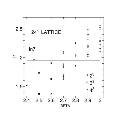
Fig. 2: Coupling constants $f_{1}$ versus $\beta$ for $2^{3},3^{3}$, and $4^{3}$ extended monopoles on $24^{4}$ lattice.

Since the action is fixed, it is possible to study energy and entropy balance of monopole loops in order to confirm the occurence of monopole condensation. If the entropy of a monopole loop exceeds the energy, the condensation of a monopole loop occurs. As done in compact QED,[21] the entropy of a monopole loop can be estimated as $\ln 7$ per unit loop length. Since monopole currents are distributed randomly in average for large $L$, interaction terms between two separate currents is expected to be canceled. That this actually happens will be shown later in the case of $T\neq 0$ QCD case. Hence the action may be approximated by the self energy part $f_{1}L$. Here dominance of currents with a unit charge is used. Since $f_{1}$ is regarded as the self energy per unit monopole loop length, the free energy per unit monopole loop length is approximated by

$$f_{1}-\ln 7.$$ (37)

If $f_{1}<\ln 7$, the entropy dominates over the energy, which means condensation of monopoles. In Fig.2, $f_{1}$ versus $\beta$ for various extended monopoles on $24^{4}$ lattice is shown in comparison with the entropy value $\ln 7$. Each extended monopole has its own $\beta$ region where the condition $f_{1}<\ln 7$ is satisfied. When the extendedness is bigger, larger $\beta$ is included in such a region. Larger extended monopoles are more important in determining the phase transition point.

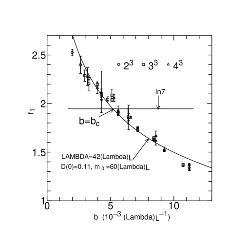
Fig. 3: Coupling constants $f_{1}$ versus $b$.

The behaviors of the coupling constants are different for different extended mono-poles. However, if we plot them versus $b=n\times a(\beta)$, we get a unique curve as in Fig.3. The coupling constants seem to depend only on $b$, not on the extendedness nor $\beta$. There is a critical $b_{c}$ corresponding to critical $\beta^{n}_{c}$, i.e., $b_{c}=na(\beta^{n}_{c})$. The monopole action may be fitted by

$$S[k] = \sum m_{0}bk_{\mu}(s)k_{\mu}(s)+\frac{1}{2}(\frac{4\pi}{g(b)})^{2}\sum k_{\mu}(s)\bar{D}(s-s^{\prime})k_{\mu}(s^{\prime}),$$ (38)

where $g(b)$ is the SU(2) running coupling constant

$$g(b)^{-2}=\frac{11}{24\pi^{2}}\ln(\frac{1}{b^{2}\Lambda^{2}})+\frac{17}{44\pi^{2}}\ln\ln(\frac{1}{b^{2}\Lambda^{2}}).$$ (39)

$\bar{D}(s)$ is a modified lattice Coulomb propagator. This form of the action is predicted theoretically by Smit and Sijs.[22] The solid line is the prediction given by the action with the parameters written in Fig.3.

Suppose the effective monopole action remains the same for any extended mono-poles larger than $4^{3}$ in the infinite volume limit. Then the finiteness of $b_{c}=na(\beta^{n}_{c})$ suggests $\beta^{n}_{c}$ becomes infinite when the extendedness $n$ goes to infinity. $SU(2)$ lattice QCD is always (for all $\beta$) in the monopole condensed and then in the color confinement phase.[1] This is one of what one wants to prove in the framework of lattice QCD.

Notice again that considering extended monopoles correponds to performing a block spin transformation on the dual lattice. The above fact that the effective actions for all extended monopoles considered are the same for fixed $b$ means that the action may be the renormalized trajectory on which one can take the continuum limit. Our results suggest the continuum monopole action takes the form (38) predicted by Smit and Sijs.[22] The simulation of the monopole action is in progress.

Shiba and Suzuki[6, 7, 8] showed furthermore that monopoles alone can reproduce the full value of the string tension in $SU(2)$ QCD. These facts strongly suggest that the monopole condensation occurs in QCD and quarks and gluons are confined due to the dual Meissner effect.

§4 Deconfinement transition in $T\neq 0$ QCD

Now let us study the role of the monopoles in the deconfinement transition in $T\neq 0$ QCD. There have been interesting data already suggesting the importance of monopoles also in $T\neq 0$ QCD. Monopole contribution to the string tension has been studied in the MA gauge also in $T\neq 0$ $SU(2)$ QCD. The string tension from the monopoles almost agrees with that from the abelian Wilson loops in the confinement phase, whereas it vanishes clearly in the deconfinement phase. The data are shown in Fig.4. The string tension from the photon part is negligibly small.

Fig. 4: Physical string tensions (circle) and spatial string tensions (square) from monopoles on $24^{3}\times 8$ lattice.

Fig. 5: Monopole Dirac string and photon contributions to Polyakov loops in the MA gauge in $SU(2)$ QCD on $16^{3}\times 4$ lattice. Total means the abelian Polyakov loops.

An abelian Polyakov loop which is written in terms of abelian link fields alone is given by a product of contributions from Dirac strings of monopoles and from photons. It has been found [11, 12] that the characteristic features of the Polyakov loops as an order parameter of the deconfinement transition are due to the Dirac string contributions alone. In Fig.5, the $SU(2)$ data in the MA gauge are plotted. The abelian Polyakov loops vanish in the confinement phase whereas they begin to rise for $\beta$ larger than the critical temperature $\beta_{c}=$ 2.298. The Dirac string contribution shows similar behaviors more drastically. The photon part has a finite contribution for both phases and it changes only slightly. The fact that monopoles are responsible for the essential feature of the Polyakov loop is found also in $U(1)$ and in $SU(3)$ in the MA gauge. In addition, a remarkable result has been found. The behavior of the abelian Polyakov loops as an order parameter and the monopole responsibility are seen also in other gauges like unitary ones. This is the first phenomena suggesting gauge independence of the ’tHooft conjecture.

4.1 The expected role of maximally extended monopoles

In $T=0$ QCD, each extended monopole has its own $\beta$ region where the entropy dominance of monopoles occurs, i.e., where the condition $f_{1}<\ln 7$ is satisfied. When the extendedness is bigger, larger $\beta$ is included in such a region. Larger extended monopoles are more important in determining the phase transition point. In the infinite-volume limit, one can adopt infinitely extended monopoles. If the situations remain unaltered even in the infinite-volume limit, one can prove that $T=0$ $SU(2)$ lattice QCD is always (for all $\beta$) in the monopole condensed and then in the color confinement phase.[1]

What happens in $T\neq 0$ QCD? It is expected that the confinement - deconfinement transition in $T\neq 0$ QCD also can be explained in terms of monopoles. Then energy and entropy balance of monopoles must be the mechanism as shown above in $T=0$ QCD. However, there is a big difference between $T=0$ and $T\neq 0$ QCD. Namely the time extent $N_{t}$ is kept finite in $T\neq 0$ case. This means that the extendedness of monopoles running in the space direction (which we call dynamical monopoles) is restricted to be finite, since monopoles are defined by a three dimensional cube perpendicular to the direction of the current. The monopole currents which contribute to the physical string tension are those running in the direction perpendicular to the Wilson loops. Because the Wilson loops are on a plane which include the time axis and a space one, dynamical monopoles are essential in the confinement mechanism. It is our expectation that the existence of the maximum size of extended dynamical monopoles is the reason there is a deconfinement phase transition at a finite value of $\beta_{c}$, i.e., $T_{c}$ in the finite temperature QCD. Here $T_{c}$ is the critical temperature.

In the following subsections, we explore what is the maximum size of extended monopoles and whether $\beta_{c}$ can be explained by balancing of energy and entropy of the maximally extended monopole loops in the MA gauge.

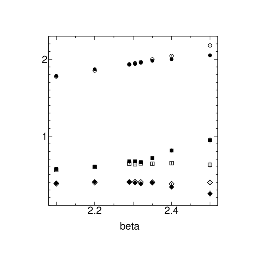
Fig. 6: Coupling constants $f_{1}$(circle), $f_{2}$(square) and $f_{3}$(diamond) versus $\beta$ on $16^{3}\times 4$ lattice for $1^{3}$ monopoles. Open symbols are the couplings connecting two space-like currents and filled ones are those connecting two time-like currents.

4.2 Monopole action in $T\neq 0$ QCD

Monopole action can be calculated from monopole current configurations similarly as in $T=0$ $SU(2)$ QCD. The partition function is expressed by Eq.(36). In contrast with the case of $T=0$ QCD, we must treat time and space directions separately. Since the number of sites in the time direction is small, we consider only up to next to the nearest quadratic couplings. Owing to the current conservation, five interaction terms are sufficient in this case. In Fig.6 the action is calculated in both the confinement and the deconfinement phases on $16^{3}\times 4$ lattices. We used 50 (100 at some points) configurations adopting $1^{3}$ monopoles. $f_{1}$ is the coupling of the self energy term $\sum_{n,\mu}(k_{\mu}(s))^{2}$, $f_{2}$ is the coupling of the term $\sum_{n,\mu}k_{\mu}(s)k_{\mu}(s+\hat{\mu})$ and $f_{3}$ is the coupling of the term, $\sum_{n,\mu\neq\nu}k_{\mu}(s)k_{\mu}(s+\hat{\nu})$. Other couplings between currents larger distance apart are much smaller. $f_{1}$ is dominant in both phases. In the deconfinement phase, the discrepancy between space-space and time-time couplings is large, whereas it is negligible in the confinement phase.

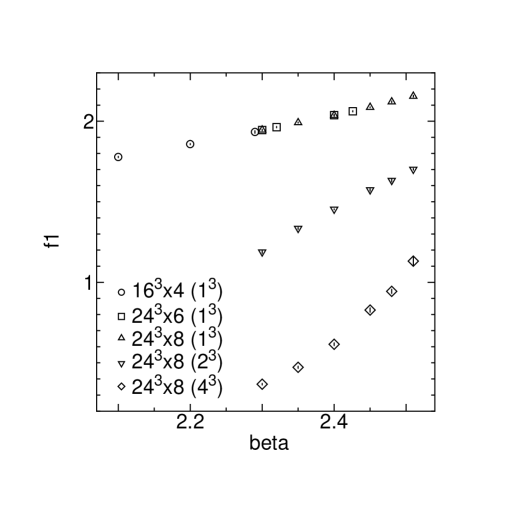
Fig. 7: Coupling constants $f_{1}$ in the confinement phase versus $\beta$ on various lattices. The parenthesized number represents the extendedness of monopoles.

$f_{1}$ of the monopole action is plotted in Fig.7 in the confinement phase on various lattices. In the confinement phase the action is independent of $N_{s}$ and $N_{t}$ ,i.e., of the lattice volume and the action obtained seems the same as that given in $T=0$ QCD.

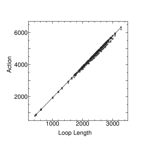
Fig. 8: The values of the total monopole action (circle), self energy term of the action (square) and $f_{1}$ times the length of a monopole loop $L$ versus monopole loop length (solid line).

Now that the energy of a monopole loop is evaluated, let us check if all terms other than the self energy are canceled because of randomness of the monopole loop distribution. In Fig.8 we compare the value of the total monopole action with that of the self energy term and also with that of $f_{1}\times L$, where $L$ is the length of a monopole loop. The length of monopole loops will be defined in detail in the next subsection. The data show that the cancellation is good and the total action is well approximated only by the self energy term. Furthermore the value of the self energy term is in fairly good agreement with $f_{1}\times L$, which suggests dominance of monopole currents with unit charge. Next, we pay attention to the entropy of a monopole loop.

4.3 Monopole loop length

Suppose that the behavior of a monopole loop is represented by non-backtracking random walks, the number of loops of length $L$ on four-dimensional large lattice behaves as $7^{L}$. The entropy of a monopole loop can be estimated as $\ln 7$ per unit loop length in $T=0$ QCD. However, the entropy of the loop in $T\neq 0$ QCD must be affected by the finiteness of the time direction and the entropy may become smaller than $\ln 7$. To estimate the entropy, we have to investigate the behavior of monopole loops carefully in $T\neq 0$ QCD.

(a)
$L$	number	$L$	number	$L$	number	$L$	number
4	708	24	4	46	1	5010	1
6	238	26	1	52	1	5012	1
8	89	28	1	100	1	5092	1
10	50	30	3	4612	1
12	33	32	4	4798	1
14	24	34	3	4822	1
16	15	36	1	4854	1
18	8	40	2	4876	1
20	9	42	1	4880	1
22	6	44	1	4940	1
(b)
$L$	number	$L$	number	$L$	number	$L$	number
2	19	10	1	1292	1	1336	1
4	14	1272	2	1302	1	1340	2
6	2	1288	1	1318	1	1348	1

Table 1: The total number of loops of length $L$ on a sample of 10 configurations on $16^{3}\times 4$ lattice at $\beta=$2.20 for $1^{3}$ monopoles (a) and $2^{3}$ monopoles (b).

First, we calculate the length of monopole loops. Bode et al.[23] studied the length of monopole loops in $U(1)$ lattice gauge theory. They found that in the confinement phase one large loop occupies the whole lattice and in the Coulomb phase it splits into several smaller pieces. We define the monopole loop length following Bode et al[23] in the MA gauge in $SU(2)$ QCD. If two closed loops occupy some sites in common, these two loops are regarded as one loop with the number of crossings. It is found that in the confinement phase, a long monopole loop exists in each configuration in addition to some short loops. The separation of long loop and other short loops is clearly seen in Table 1, where the data are obtained from 10 configurations at $\beta=$ 2.20 on $16^{3}\times 4$ lattice. Note that the number of long loop is equal to the number of configurations. In this case, $\beta_{c}$ is 2.298. For $\beta<\beta_{c}$ long monopole loops have a characteristic length at each $\beta$ and the long loops become shorter or split into a few parts around $\beta_{c}$. In the deep deconfinement region, no long loop exists and all monopole loops are short. These results are consistent with those in the $U(1)$ case.[23]

(a)
$\beta$	2.35	2.45	2.48	2.51	2.53	2.57	2.63	2.70
$\langle L\rangle$	4980	2205	1710	838	479	148	69	35
$\langle$crossing$\rangle$	1120	316	219	94	50	13	5	2
charge 1	97.62	98.67	98.88	99.04	99.07	99.52	99.29	99.27
charge 2	2.36	1.32	1.12	0.96	0.93	0.48	0.70	0.73
charge 3	0.02	0.01	0.00	0.00	0.00	0.00	0.00	0.00
charge 4	0.00	0.00	0.00	0.00	0.00	0.00	0.00	0.00
(b)
$\beta$	2.35	2.45	2.48	2.51	2.53	2.57	2.63	2.70
$\langle L\rangle$	1140	700	605	450	357	169	54	21
$\langle$crossing$\rangle$	714	320	246	157	110	45	12	3
charge 1	81.07	90.98	92.10	93.85	94.92	95.92	96.44	98.54
charge 2	16.98	8.43	7.69	5.91	5.02	4.02	3.36	1.45
charge 3	1.87	0.57	0.20	0.23	0.06	0.06	0.19	0.00
charge 4	0.09	0.03	0.01	0.01	0.00	0.00	0.00	0.00

Table 2: The length of the longest loop, the number of crossings and the ratio (percent) of the number of multicharged monopole currents to the total number of monopole currents in the case of $2^{3}$-extended monopoles (a) and that of $4^{3}$-extended monopoles (b) on $24^{3}\times 8$ lattice. The numbers are averages over 30 configurations.

In Table 2, the $\beta$-dependence of the loop length $\langle L\rangle$, the number of crossings and the ratio of the number of multicharged currents to the number of the total currents are shown. Those quantities are calculated from 30 configurations for two different sized monopoles on $24^{3}\times 8$ lattice. $\beta_{c}$ is 2.51 on this lattice. The number of crossings is small in the case of $2^{3}$ monopole, whereas it is not so small in the case of $4^{3}$ monopole. The monopole currents with a unit charge are dominant for both extended monopoles, which is consistent with that $f_{1}$ is dominant on the monopole action. In the case of $4^{3}$ monopole, $\langle L\rangle$ exceeds the site number of the renormarized lattice for $\beta<\beta_{c}$, whereas they are nearly equal around $\beta_{c}$. In the case of $2^{3}$ monopole $\langle L\rangle$ is smaller than the number of the sites.

Recently, Ejiri et al.[9, 10] have evaluated the string tension derived from long and short monopole loops separately. They have found that the long loops alone can reproduce the full value of the string tension in spite of the fact that only a few percents of a total dual links are occupied by the long loop. Other short loops do not contribute to the string tension. This suggests that the long loops are essential in the deconfinement transition.

4.4 The distribution of monopole currents

Now we pay attention to long loops and investigate the distribution of monopole currents contained in a long loop. Even the longest loop occupies only about 10 percent of the total dual links. Does the long loop spread uniformly through the lattice or not? In Ref.[23]), it is filling up the whole lattice in compact QED.

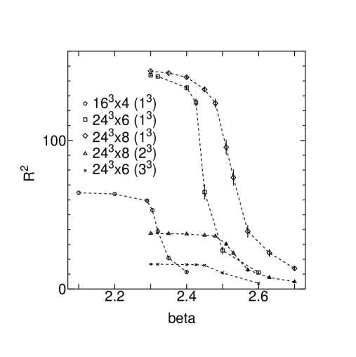
Fig. 9: $R^{2}$ versus $\beta$ on various lattices. The number in the parentheses represents the extendedness of monopoles.

We calculate the mean square of the distance from the center as follows:

$$R^{2}=\frac{1}{L}\sum_{i}(\vec{r}_{i}-\vec{R}_{G})^{2},$$ (40)

where $L$ is the length of the monopole loop, $\vec{r}_{i}$ is the position of a monopole current and $\vec{R}_{G}$ is the position of the center. If the monopole currents exist uniformly on the $N_{s}^{3}\times N_{t}$ lattice, $R^{2}$ should be evaluated as

$$\frac{1}{N_{s}^{3}N_{t}}\int^{N_{s}/2}_{-N_{s}/2}dx\int^{N_{s}/2}_{-N_{s}/2}dy\int^{N_{s}/2}_{-N_{s}/2}dz\int^{N_{t}/2}_{-N_{t}/2}dt(x^{2}+y^{2}+z^{2}+t^{2})=\frac{N_{s}^{2}}{4}+\frac{N_{t}^{2}}{12}.$$ (41)

In the case of $n^{3}$ extended monopole, $R^{2}$ should be

$$\frac{(N_{s}/n)^{2}}{4}+\frac{(N_{t}/n)^{2}}{12}.$$ (42)

Our data of $R^{2}$ are shown in Fig.9. $\beta_{c}$ is 2.426 in the case of $N_{t}=6$ and $\beta_{c}$ is 2.51 in the case of $N_{t}=8$. In the confinement phase, the data almost coincide with the expected values (42). For example, $R^{2}$ is expected to be 147 in the case of $1^{3}$ monopole on $24^{3}\times 6$ lattice and in the case of $3^{3}$ monopole $R^{2}$ is expected to be 16. The long monopole loop is almost uniformly distributed in the whole lattice in the confinement phase. In the deconfinement phase $R^{2}$ starts to decrease rapidly above $\beta_{c}$. In the case of extended monopoles the uniformity is better than in the $1^{3}$ case for $\beta\leq\beta_{c}$.

4.5 Monopole effective size

Assuming that crossings of the loop are ignored, an $n^{3}$ monopole loop seems to spread almost uniformly through the whole lattice for $\beta\leq\beta_{c}$. Considering that almost all magnetic charge is $\pm 1$ and that the loop length is rather restricted in comparison with all link numbers $4\times N_{s}^{3}\times N_{t}$, there appears to work some repulsive force between currents. To study the force, we may define an effective size of monopoles as follows:

$$l^{3}(n)=\frac{(N_{s}/n)^{3}\times(N_{t}/n)}{\langle L(n)\rangle},$$ (43)

where the numerator is the volume of the renormalized lattice of $n^{3}$ extended monopoles and the denominator is the length of the monopole loop in the renormalized lattice unit. For $\beta>\beta_{c}$ the distribution of monopole currents is not uniform as seen in the previous subsection. In this case we assume that the distribution is uniform in the region restricted to $2R$ in each spatial direction and $N_{t}$ in the time direction. Note that $2R$ is still larger than $N_{t}$ near $\beta_{c}$. Hence the effective renormalized volume which is occupied by the longest loop may be given by $(2R/n)^{3}\times(N_{t}/n)$. $l(n)$ represents the range affected by one of the $n^{3}$ monopole world line. If the monopole current with a range $l(n)$ exists on a link, the nearest current could be put on links more apart than $l(n)$. The $n^{3}$ extended monopole current with a range $l(n)$ seems to have an exclusion volume $l(n)^{4}$ in the renormalized lattice.

Considering the exclusion volume, the entropy of monopoles may be discussed, in the case of $n^{3}$ extended monopoles having the range $l(n)$, not on the whole renormalized lattice but on a reduced lattice

$$\frac{(N_{s}/n)^{3}\times(N_{t}/n)}{N(l)^{4}}\quad({\rm for}\beta\leq\beta_{c}),$$ (44)

where $N(l)$ is an integer depending on $l(n)$. It seems natural to adopt $N(l)=[l(n)]+1$, where the symbol $[l(n)]$ is the integer not exceeding $l(n)$. Monopoles are seen as if they were running only on the reduced lattice.

Fig. 10: $l(n)$ versus $\beta$ for $1^{3}$ monopoles on $16^{3}\times 4$ lattice. The dotted vertical line denotes $\beta_{c}$.

Fig. 11: $l(n)$ versus $\beta$ for $1^{3}$ (circle) and $3^{3}$ (square) monopoles on $24^{3}\times 6$ lattice. The dotted vertical line denotes $\beta_{c}$.

Fig. 12: $l(n)$ versus $\beta$ for $1^{3}$ (circle), $2^{3}$ (triangle) and $4^{3}$ (diamond) monopoles on $24^{3}\times 8$ lattice. The dotted vertical line denotes $\beta_{c}$.

$l(n)$ are shown in Figs.10-12. In the case of $1^{3}$ monopole on $16^{3}\times 4$ lattice shown in Fig.10, we see that $l(n=1)$ is less than 2 for $\beta<\beta_{c}$ and approaches 2 at $\beta_{c}$. $l(n=1)$ approaches 3 from below as $\beta\to\beta_{c}$ in the case of $1^{3}$ monopole on $24^{3}\times 6$ lattice, whereas $l(n=3)\leq 1$ in the case of $3^{3}$ as seen from Fig.11. The same regularity exists also for any extended monopole on $24^{3}\times 8$ lattice shown in Fig.12. It is stressed that $l(n)$ is always less than or equal to $N_{t}/(2n)$ for $\beta\leq\beta_{c}$. This leads us to that the reduced lattice always has a time extent $2=(N_{t}/n)/(N_{t}/(2n))$ for $\beta\leq\beta_{c}$. Then the entropy of a $n^{3}$ extended monopole loop for any $n$ should be calculated always on a reduced lattice with the time extent 2 for $\beta\leq\beta_{c}$. This means that the entropy of a $n^{3}$ monopole is the same for any $n$, since the reduced lattice is the same for any extendedness $n$ if the original lattice is the same.

4.6 The entropy of a monopole loop and the deconfinement transition

In the previous subsection, we have seen that the entropy of a $n^{3}$ monopole is the same for any $n$ if the original lattice is the same. However, the action is different for different extended monopoles at fixed $\beta$. Since the entropy is equal, larger extended monopoles are more important to fix the point of the deconfinement transition as seen from Fig.7.

What is the maximum size of extended monopole? To define dynamical monopole currents which are important, the renormalized lattice should have at least two independent lattice sites in the time direction. This means that the maximum size $n_{max}$ of dynamical extended monopoles is $N_{t}/2$. From Figs.10-12, we see the maximally extended monopoles have always $l(n_{max})\leq 1$ for $\beta\leq\beta_{c}$. The reduced lattice is the same as the renormalized one for $\beta\leq\beta_{c}$ in the case of the maximally extended monopole.

What is the entropy of a long monopole loop on the reduced lattice with $N_{t}=2$ ? As shown above, a long monopole loop seems to behave like a random walk with a stronger repulsive condition than a simple non-backtracking. However to know the condition correctly is not simple. Moreover, the number of crossing increases as extendedness becomes large. The entropy is very difficult to estimate contrary to the case in $T=0$ $SU(2)$ QCD.

Fig. 13: The histograms of the length of $2^{3}$ monopole loops on $12^{3}\times 4$ lattices.

Therefore, let us investigate the entropy by a histogram method using Monte Carlo simulations. It is easy to get the histogram of the length of monopole loops from many configurations generated in the Monte Carlo simulations. The lengths of $2^{3}$ extended monopole loops are measured on $12^{3}\times 4$ lattice, since they are the maximally extended monopole in this case. The histogram is obtained from 3000 configurations as shown in Fig.13. $\beta_{c}$ is 2.298 on the lattice. The vertical line represent the frequency of length. The distribution of the long monopole loops seems to be Gaussian.

The number of loops of length $L$ through a given point goes asymptotically like $\mu^{L}$ irrespective of the conditions of random walks.[24] Hence the distribution of the long loop length may be fitted by the following form

$$-aL^{2}+bL+c,\quad b=\ln\mu-f_{1},$$ (45)

where $f_{1}$ comes from the self energy term in the monopole action and c is a constant. The term of $-aL^{2}$ should come from all other terms than the self energy and it is very small as seen from Fig.8. But the term is important because it suppresses proliferation of monopole loops in the condensed phase. The linear term may determine the entropy $\ln\mu$.

$\beta$	a	b
$2.10$	$1.80\times 10^{-4}$	$2.93\times 10^{-1}$
$2.20$	$1.41\times 10^{-4}$	$1.76\times 10^{-1}$
$2.30$	$6.65\times 10^{-5}$	$4.93\times 10^{-2}$
$2.35$	$5.70\times 10^{-5}$	$2.31\times 10^{-2}$

Table 3: Least square fitting of the histogram for $\beta=2.10$, $2.20$, $2.30$ and $2.35$.

We plot in Table 3 the values of the parameters of the Gaussian fit to the data at $\beta=2.1\sim 2.35$, where the Gaussian shape is seen. We see from the table that the linear term at $\beta_{c}=2.298$ is already small and it almost vanishes around $\beta=$ 2.35. If the balancing of energy and entropy of maximally extended monopole is the origin of the deconfinement transition, the predicted critical coupling is $\beta_{c}\sim 2.35$ which is near to the actual critical coupling $\beta_{c}=2.298$. Considering the finite size effects near $\beta_{c}$, the agreement is fairly good.

From the fit, one can estimate roughly the value of the entropy using the values of $f_{1}(\beta)$, i.e., $f_{1}(2.35)\sim 1.3$ and $f_{1}(2.298)\sim 1.16$. We get $1.16\leq\ln\mu\leq 1.3$.

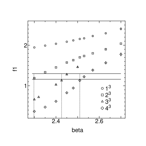
Fig. 14: Coupling constant $f_{1}$ for various extended monopoles. The dotted vertical lines denote $\beta_{c}$ for $N_{t}=4,6$ and $8$ from the left.

In Fig.14, we plot $f_{1}$ for maximally extended monopoles on various lattices in comparison with the entropy estimated above. We find that the balancing of the energy and the entropy of the monopoles can explain the transition points of all lattices approximately. There are, however, many things to be studied. Nevertheless, it is very interesting that the deconfinement transition can be understood roughly by the simple idea of balancing of energy and entropy of monopole loops in $T\neq 0$ $SU(2)$ QCD.

§5 Conclusion and remarks

1. In $T\neq 0$ QCD, it is found that a long monopole loop exists in each configuration and all other loops are short in the confinement phase. They distribute almost uniformly in the confinement phase. Table 1 shows that the number of short loops decrease in the case of $2^{3}$ monopoles in comparison with the case of $1^{3}$ monopoles. To study the continuum limit, we have to make the time extent $N_{t}$ large. Then large extended monopoles are important and short loops would disappear rapidly. It is expected that long monopole loops alone are responsible for the confinement mechanism of quarks. This is consistent with the result that the string tension is reproduced only by long monopole loops.[9, 10]

2. Almost all magnetic charge is $\pm 1$ and the loop length is rather restricted in comparison with all link numbers of lattice. There appears to work some repulsive force between currents, so that monopoles may have an exclusion volume around them. Considering the exclusion volume determined from the distribution data, we have derived that the entropy of extended monopoles may be independent of the extendedness if the original lattice is the same.

3. In $T\neq 0$ QCD there exists a maximally extended ($(N_{t}/2)^{3}$) monopole contrary to the case of $T=0$ $SU(2)$ QCD where larger and larger extended monopoles become important. The critical temperature becomes necessarily finite. Balancing of energy and entropy of the maximally extended monopoles can explain roughly the deconfinement transition of various lattices. However more intensive studies are needed to clarify the transition mechanism definitely. Especially, the finite size effect near $\beta_{c}$ should be clarified in details.

References

- [1] G. ’tHooft, Nucl. Phys. B190 (1981), 455.
-
[2]
A.S. Kronfeld , Phys. Lett.
B198 (1987), 516.
A.S. Kronfeld , Nucl.Phys. B293 (1987), 461. - [3] T. Suzuki and I. Yotsuyanagi, Phys. Rev. D42 (1990), 4257; Nucl. Phys. B(Proc. Suppl.) 20 (1991), 236.
- [4] T. Suzuki, Nucl. Phys. B(Proc. Suppl.) 30 (1993), 176 and references therein.
- [5] S. Hioki , Phys. Lett. B272 (1991), 326.
- [6] H.Shiba and T.Suzuki, Kanazawa University, Report No. Kanazawa 93-10, 1993 (unpublished).
- [7] H.Shiba and T.Suzuki, Nucl. Phys. B(Proc. Suppl.) 34 (1994), 182 .
- [8] H.Shiba and T.Suzuki, Phys. Lett. B333 (1994), 461.
- [9] S.Ejiri, S.Kitahara, Y.Matsubara and T.Suzuki, Kanazawa University Report KANAZAWA 94-14, 1994, to appear in Physics Letters B.
- [10] S.Ejiri, S.Kitahara, Y.Matsubara and T.Suzuki, Talk at Lattice 94, to appear in Nucl. Phys. B(Proc. Suppl.).
- [11] T. Suzuki , Kanazawa University Report KANAZAWA 94-15, 1994, to appear in Physics Letters B.
- [12] Y.Matsubara , Talk at Lattice 94, to appear in Nucl. Phys. B(Proc. Suppl.).
- [13] H.Shiba and T.Suzuki, Kanazawa University Report KANAZAWA 93-09, 1993 (unpublished).
- [14] H.Shiba and T.Suzuki, Kanazawa University Report KANAZAWA 94-11, 1994, to appear in Physics Letters B.
- [15] H.Shiba and T.Suzuki, Kanazawa University Report KANAZAWA 94-12, 1994.
- [16] T. Suzuki and H. Shiba, Talk at Lattice 94, to appear in Nucl. Phys. B(Proc. Suppl.).
- [17] T.L. Ivanenko , Phys. Lett. B252 (1990), 631.
- [18] J. Arafune , Jour. Math. Phys. 16 (1975), 433.
- [19] T.A. DeGrand and D. Toussaint, Phys. Rev. D22 (1980), 2478.
- [20] R.H. Swendsen,Phys. Rev. Lett. 52 (1984), 1165; Phys. Rev. B30 (1984), 3866, 3875.
- [21] T.Banks , Nucl. Phys. B129 (1977), 493.
- [22] J. Smit and A.J. van der Sijs, Nucl. Phys. B355 (1991), 603.
- [23] A. Bode, Th. Lippert and K. Schilling, Nucl. Phys. B(Proc. Suppl.) 34 (1994), 549.
- [24] P.J. Gans, Jour. Chem. Phys. 42 (1965), 4159 and references therein.