Monopole action and condensation in SU(2) QCD

Abstract

An effective monopole action for various extended monopoles is derived from vacuum configurations after abelian projection in the maximally abelian gauge in $SU(2)$ QCD. The action appears to be independent of the lattice volume. Moreover it seems to depend only on the physical lattice spacing of the renormalized lattice, not on $\beta$. Entropy dominance over energy of monopole loops is seen on the renormalized lattice with the spacing $b>b_{c}\simeq 5.2\times 10^{-3}\Lambda_{L}^{-1}$. This suggests that monopole condensation always (for all $\beta$) occurs in the infinite-volume limit of lattice QCD.

To clarify color confinement mechanism is still important in particle physics and the effect dual to the Meissner effect is believed to be the mechanism [1, 2]. This picture is realized in the confinement phase of lattice compact QED[3, 4, 5].

To apply the idea to QCD, we have to find a color magnetic quantity inside QCD. The ’tHooft idea of abelian projection of QCD[6] is very interesting. The abelian projection of QCD is to extract an abelian gauge theory by performing a partial gauge-fixing such that the maximal abelian subgroup remains unbroken. Then QCD can be regarded as an abelian gauge theory with magnetic monopoles and electric charges. ’t Hooft conjectured that the condensation of the abelian monopoles is the confinement mechanism in QCD[6].

There are, however, infinite ways of extracting such an abelian theory out of QCD. It seems important to find a good gauge in which the conjecture is seen to be realized in a coupling region where reliable calculations can be done at present. A gauge called maximally abelian (MA) gauge has been shown to be very interesting [7, 8, 9]. In the MA gauge, there are phenomena which may be called abelian dominance [8, 10]. Moreover the monopole currents $k_{\mu}(s)$ defined similarly as in compact QED[5] are seen in the MA gauge to be dense and dynamical in the confinement phase, while dilute and static in the deconfinement phase [9]. Especially the string tension can be reproduced by the monopole contributions alone[11, 12].

Although these data support the ’tHooft conjecture, there is not a direct evidence of abelian monopole condensation in the QCD vacuum. In the case of compact QED, the exact dual transformation can be done and leads us to an action describing a monopole Coulomb gas, when one adopt the partition function of the Villain form [4, 13, 14, 15]. Monopole condensation is shown to occur in the confinement phase from energy-entropy balance of monopole loops.

In the case of QCD, however, we encounter a difficulty in performing the exact dual transformation. Hence we tried to do it numerically first by fixing an effective U(1) action. Namely, the abelian dominance suggests that a set of $U(1)$ invariant operators are enough to describe confinement after the abelian projection. Then there must exist an effective $U(1)$ action describing confinement. As reported in [9], however, to derive a compact form of such a $U(1)$ action in terms of abelian link variables was unsuccessful in the scaling region. Here we propose a method to directly determine a monopole action numerically from the vacuum configurations of monopole currents given by Monte-Carlo simulations in the MA gauge[16, 17]. This can be done by extending the Swendsen method[18] which was developed in the studies of the Monte-Carlo renormalization group. We have shown recently that the method is successfully applied to compact QED[19]. When applied to SU(2) QCD in the MA gauge, it is suggested that entropy dominance over energy and then monopole condensation always occur in the infinite-volume limit of lattice QCD. A preliminary report was published in [16, 17].

The MA gauge is given on a lattice by performing a local gauge transformation

$$\widetilde{U}(s,\mu)=V(s)U(s,\mu)V^{-1}(s+\hat{\mu})$$ (1)

such that a quantity

$$R=\sum_{s,\hat{\mu}}{\rm Tr}\Big{(}\sigma_{3}\widetilde{U}(s,\mu)\sigma_{3}\widetilde{U}^{\dagger}(s,\mu)\Big{)}$$ (2)

is maximized[7]. In the continuum limit, this corresponds to a gauge $(\partial_{\mu}+igA_{\mu}^{3})(A_{\mu}^{1}-iA_{\mu}^{2})=0.$ Such a gauge fixing keeps a residual U(1) invariance.

After the gauge fixing is done, an abelian link gauge field is extracted from the $SU(2)$ link variables as follows;

$$\widetilde{U}(s,\mu)=\left(\begin{array}[]{cc}(1-|c(s,\mu)|^{2})^{1/2}&-c^{*}(s,\mu)\\ c(s,\mu)&(1-|c(s,\mu)|^{2})^{1/2}\end{array}\right)\left(\begin{array}[]{cc}u(s,\mu)&0\\ 0&u^{*}(s,\mu)\end{array}\right),$$ (7)

where $u(s,\mu)=\exp(i\theta(s,\mu))$ represents the abelian link field and $c(s,\mu)$ corresponds to charged matter fields.

A plaquette variable $\theta_{\mu\nu}(s)\in(-4\pi,4\pi)$ is given by a link angle $\theta(s,\mu)\in[-\pi,\pi)$ as $\theta_{\mu\nu}(s)=\theta(s,\mu)+\theta(s+\hat{\mu},\nu)-\theta(s+\hat{\nu},\mu)-\theta(s,\nu)$. The plaquette variable $\theta_{\mu\nu}(s)$ can be decomposed into

$$\theta_{\mu\nu}(s)=\bar{\theta}_{\mu\nu}(s)+2\pi m_{\mu\nu}(s),$$ (8)

where $\bar{\theta}_{\mu\nu}(s)\in[-\pi,\pi)$ is interpreted as the electromagnetic flux through the plaquette and $m_{\mu\nu}(s)$ can be regarded as a number of the Dirac string penetrating the plaquette. DeGrand and Toussaint[5] defined a monopole current as

$$k_{\mu}(s) = \frac{1}{2}\epsilon_{\mu\nu\rho\sigma}\partial_{\nu}m_{\rho\sigma}(s+\hat{\mu}),$$ (9)

where $\partial$ is the forward difference. It is defined on a link of the dual lattice (the lattice with origin shifted by half a lattice distance all in four directions). $k_{\mu}(s)$ can take only the values $0,\pm 1,\pm 2$ and satisfies

$$\partial^{\prime}_{\mu}k_{\mu}(s)=0,$$ (10)

where $\partial^{\prime}$ is the backward derivative on the dual lattice.

Long-distance behaviors are expected to be important in the confinement phase of QCD. Hence we consider extended monopoles of the type-2 [20] as shown in Fig. 1. The $n^{3}$ extended monopole of the type-2 has a total magnetic charge inside the $n^{3}$ cube and is defined on a sublattice with the spacing $b=na$, $a$ being the spacing of the original lattice.

$$k_{\mu}^{(n)}(s) = \frac{1}{2}\epsilon_{\mu\nu\rho\sigma}\partial_{\nu}m_{\rho\sigma}^{(n)}(s+\hat{\mu})$$ (11)

$$= \sum_{i,j,l=0}^{n-1}k_{\mu}(ns+(n-1)\hat{\mu}+i\hat{\nu}+j\hat{\rho}+l\hat{\sigma}),$$ (12)

$$m_{\rho\sigma}^{(n)}(s) = \sum_{i,j=0}^{n-1}m_{\rho\sigma}(ns+i\hat{\rho}+j\hat{\sigma}).$$ (13)

The definition of the type-2 extended monopoles corresponds to making a block spin transformation of the monopole currents with the scale factor $n$. We call the sublattice as a renormalized lattice. We derived the coupling constants for $1^{3},2^{3},3^{3}$, and $4^{3}$ extended monopoles.

A theory of monopole loops is given in general by the following partition function

$$Z=(\prod_{s,\mu}\sum_{k_{\mu}(s)=-\infty}^{\infty})(\prod_{s}\delta_{\partial^{\prime}_{\mu}k_{\mu}(s),0})\exp(-S[k]),$$ (14)

where $k_{\mu}(s)$ is the conserved integer-valued monopole current defined above in (9) or (11) and $S[k]$ is a monopole action describing the theory. Consider a set of all independent operators which are summed up over the whole lattice. We denote each operator as $S_{i}[k]$. Then the action can be written as a linear combination of these operators:

$$S[k]=\sum_{i}f_{i}S_{i}[k],$$ (15)

where $f_{i}$ are coupling constants.

Let us now determine the monopole action using the monopole current ensemble which are calculated from vacuum configurations generated by Monte-Carlo simulations. Since the dynamical variables here are $k_{\mu}(s)$ satisfying the conservation rule, it is necessary to extend the original Swendsen method[18]. Consider a plaquette $(s^{\prime},\hat{\mu^{\prime}},\hat{\nu^{\prime}})$ instead of a link on the dual lattice. Introducing a new set of coupling constants $\{\tilde{f}_{i}\}$, define

$$\bar{S}_{i}[k]=\frac{\sum_{M=-\infty}^{\infty}S_{i}[k^{\prime}]\exp(-\sum_{i}\tilde{f}_{i}S_{i}[k^{\prime}])}{\sum_{M=-\infty}^{\infty}\exp(-\sum_{i}\tilde{f}_{i}S_{i}[k^{\prime}])},$$ (16)

where $k^{\prime}_{\mu}(s)=k_{\mu}(s)+M(\delta_{s,s^{\prime}}\delta_{\mu\mu^{\prime}}+\delta_{s,s^{\prime}+\hat{\mu}^{\prime}}\delta_{\mu\nu^{\prime}}-\delta_{s,s^{\prime}+\hat{\nu}^{\prime}}\delta_{\mu\mu^{\prime}}-\delta_{s,s^{\prime}}\delta_{\mu\nu^{\prime}}).$ When all $\tilde{f}_{i}$ are equal to $f_{i}$, one can prove an equality $\langle\bar{S}_{i}\rangle=\langle S_{i}\rangle$, where the expectation values are taken over the above original action with the coupling constants $\{f_{i}\}$:

$$\langle O[k]\rangle=\frac{(\prod_{s,\mu}\sum_{k_{\mu}(s)=-\infty}^{\infty})(\prod_{s}\delta_{\partial^{\prime}_{\mu}k_{\mu}(s),0})O[k]\exp(-\sum_{i}f_{i}S_{i}[k])}{(\prod_{s,\mu}\sum_{k_{\mu}(s)=-\infty}^{\infty})(\prod_{s}\delta_{\partial^{\prime}_{\mu}k_{\mu}(s),0})\exp(-\sum_{i}f_{i}S_{i}[k])}.$$ (17)

When there are some $\tilde{f}_{i}$ not equal to $f_{i}$, one may expand the difference as follows

$$\langle\bar{S}_{i}-S_{i}\rangle=\sum_{j}\langle\overline{S_{i}S_{j}}-\bar{S}_{i}\bar{S}_{j}\rangle(f_{j}-\tilde{f}_{j}),$$ (18)

where only the first order terms are written down. This allows an iteration scheme for determination of the unknown constants $f_{i}$. For more details, see [19] where (18) is derived explicitly and is applied to compact QED.

Practically we have to restrict the number of interaction terms. We adopted 12 types of quadratic interactions listed in Table I in most of these studies. To check the validity of the truncation, we also included more quadratic and even quartic interactions in some cases, but found little difference.

Monte-Carlo simulations were done on $8^{4},12^{4},14^{4},16^{4},18^{4},20^{4}$, and $24^{4}$ lattices for $0<\beta\leq 3.0$.

Our results are summarized in the following.

1. The coupling constants $f_{1}\sim f_{5}$ for $1^{3}$ monopoles are plotted (white symbol) for small $\beta$ in Fig. 2. As shown in [9], an effective $U(1)$ action is determined for small $\beta$. It takes a Wilson $U(1)$ action with the effective coupling constant $\beta_{w}=\beta/2$. In Fig. 2, we have also plotted the data (black symbol) obtained in the case of the Wilson $U(1)$ action[19] with the coupling constant substitution. Equivalence of the two theories for small $\beta$ is seen also in the form of the monopole action.

2. For $\beta\geq 2.4$, extended monopoles are considered. The coupling constants $f_{i}$ are fixed for not so large value of $b$ ,i.e., $b<1.3\times 10^{-2}(\Lambda_{L})^{-1}$. The first important observation is that the coupling constants determined are almost independent of the lattice volume as seen from Fig. 3. We see $f_{1}$ is dominant and the coupling constants decrease rapidly as the distance between the two monopole currents increases.

3. Since the monopole action is determined, let us consider energy-entropy balance of monopole loops as done in compact QED[4]. Monopole world lines form closed loops on the dual lattice. Define $n_{L}[k]$ as the number of monopole loops of length $L$ in a monopole configuration $\{k_{\mu}(s)\}$. The contribution of monopole loops of length $L$ is represented by the average of $n_{L}[k]$ :

   $$\langle n_{L}[k]\rangle=\frac{\sum_{\{k\}}n_{L}[k]e^{-S[k]}}{\sum_{\{k\}}e^{-S[k]}},$$ (19)

   where

   $$\sum_{\{k\}}=(\prod_{s,\mu}\sum_{k_{\mu}(s)=-\infty}^{\infty})(\prod_{s}\delta_{\partial^{\prime}_{\mu}k_{\mu}(s),0}).$$ (20)

   Monopole loops of length $L$ take various forms. Choose a monopole loop $C_{L}$ of length $L$ and define

   $$\delta_{C_{L}}[k]=\left\{\begin{array}[]{ll}1&\mbox{if $C_{L}\in\{k\}$}\\ 0&\mbox{otherwise\ . }\end{array}\right.$$ (21)

   $n_{L}[k]$ is written as

   $$n_{L}[k]=\sum_{C_{L}}\delta_{C_{L}}[k],$$ (22)

   where $\sum_{C_{L}}$ denotes the sum over all loops of length $L$. Then the average (19) is

   $$\langle n_{L}[k]\rangle=\sum_{C_{L}}\langle\delta_{C_{L}}[k]\rangle.$$ (23)

   $\langle\delta_{C_{L}}[k]\rangle$ depends not only on the loop length $L$ but also on the shape of $C_{L}$.

   One may define the ’energy’ $E(L)$ of monopole loops of length $L$ as the average of $\langle\delta_{C_{L}}[k]\rangle$ over all loops of length $L$:

   $$e^{-E(L)} = \frac{\sum_{C_{L}}\langle\delta_{C_{L}}[k]\rangle}{\sum_{C_{L}}1},$$ (24)

   $$\langle\delta_{C_{L}}[k]\rangle = \frac{\sum_{\{k\}}\delta_{C_{L}}[k]e^{-S[k]}}{\sum_{\{k\}}e^{-S[k]}}.$$ (25)

   Then we get

   $$\langle n_{L}[k]\rangle=\rho(L)e^{-E(L)},$$ (26)

   where $\rho(L)=\sum_{C_{L}}1$ is the total number of monopole loops of length $L$ on a dual lattice and ln$\rho(L)$ may be regarded as the ’entropy’ of monopole loops of length $L$.

   Now we write

   $$\langle\delta_{C_{L}}[k]\rangle=e^{-S(C_{L})}\times\frac{\sum_{\{k\}}\delta_{C_{L}}[k]e^{-S[k]+S(C_{L})}}{\sum_{\{k\}}e^{-S[k]}},$$ (27)

   where $S(C_{L})$ is the contribution of a loop $C_{L}$ alone to the monopole action. For large $L$, monopole currents in a loop are distributed randomly in average. If the action consists of quadratic terms alone as assumed in our analysis, interaction terms between different currents would cancel. $S(C_{L})$ may be approximated by the self-energy part:

   $$S(C_{L})\sim f_{1}\times L,$$ (28)

   where we assumed the dominance of currents with a unit charge $|k_{\mu}(s)|=1$.

   On the otherhand, $\sum_{\{k\}}\delta_{C_{L}}[k]e^{-S[k]+S(C_{L})}$ has two types of contributions, i.e., 1)those from other loops in the presence of $C_{L}$ and 2)the interactions between $C_{L}$ and other loops. The latter may be cancelled again from randomness when $L$ is large. When we fix $C_{L}$ and make the lattice volume larger, the ratio of the number of links occupied by $C_{L}$ to total link number becomes smaller. Hence the $C_{L}$ dependence of the former may be negligible in the infinite-volume limit. We may approximate for large $L$

   $$\langle\delta_{C_{L}}[k]\rangle\propto e^{-f_{1}L},$$ (29)

   which leads to

   $$E(L)\sim f_{1}L+const.$$ (30)

   If we consider non-backtracking random walks on a four dimensional dual lattice, the number of loops of length $L$ through a given site behaves asymptotically as $7^{L}$ for large $L$. We get

   $$\rho(L)\propto 7^{L}.$$ (31)

   From (30) and (31), we obtain

   $$\langle n_{L}[k]\rangle\propto e^{(\ln 7-f_{1})L}$$ (32)

   for large $L$. If $f_{1}<$ ln7, the ’entropy’ dominates over the ’energy’ and the long monopole loops become dominant. Namely the monopole condensation occurs. The same thing happens also in compact QED[4].

   We plot $f_{1}$ versus $\beta$ for various extended monopoles on $24^{4}$ lattice in comparison with the entropy value ln7 for the infinite volume in Fig. 4. Each extended monopole has its own $\beta$ region where the condition $f_{1}<$ ln7 is satisfied. When the extendedness is bigger, larger $\beta$ is included in such a region.

4. The behaviors of the coupling constants are different for different extended monopoles. But if we plot them versus $b$ , we get a unique curve as in Figs. 5, 6 and 7. The coupling constants seem to depend only on $b$, not on the extendedness nor $\beta$. This suggests the existence of the continuum limit and the monopole action in the continuum may be similar to that given here. From Fig. 5, we see the self-energy per monopole loop length $f_{1}$ on the renormalized lattice decreases as the length scale $b$ increases. A critical length $b_{c}\sim 5.2\times 10^{-3}(\Lambda_{L})^{-1}$ exists at which the $f_{1}$ value crosses the ln7 line.

   Together with the first observation of the volume independence, we may get the following important conclusion in the infinite-volume limit. One can take always (for all $\beta$) a renormalized lattice with a spacing $b>b_{c}$ by making a block spin transformation of the monopole currents with a sufficiently large scale factor. Hence the QCD vacuum in the infinite-volume limit of lattice QCD is always (for all $\beta$) in the monopole condensed phase. This is the most important observation of this report.

5. What is the meaning of the critical length $b_{c}$? When the lattice distance $b$ of the renormalized lattice is larger than the critical length $b_{c}$, the condensation of monopole loops is shown from the above ’energy-entropy’ balance. If monopoles are physical quantities, it must have a finite energy and a finite physical size $R_{m}$. When the lattice distance $b$ is less than the physical monopole size $R_{m}$, one can not regard monopoles as a point particle running a world line on such a renormalized lattice. Hence the ’energy’ and the ’entropy’ of such monopoles can not be represented as in (30) and (31). The condition $f_{1}<$ ln7 can not be applicable to such monopoles. The above consideration suggests $R_{m}\sim O(b_{c})$.

6. Using the data of $f_{i}$, we try to fix the explicit form of the monopole action. Although the coupling constants for largely separated currents are too small with large errors, the monopole action may be fitted by the action predicted theoretically by Smit and Sijs[15]:

   $$S[k] = \sum m_{0}bk_{\mu}(s)k_{\mu}(s)+\frac{1}{2}(\frac{4\pi}{g(b)})^{2}\sum k_{\mu}(s)\bar{D}(s-s^{\prime})k_{\mu}(s^{\prime}),$$ (33)

   where $g(b)$ is the SU(2) running coupling constant

   $$g(b)^{-2}=\frac{11}{24\pi^{2}}\ln(\frac{1}{b^{2}\Lambda^{2}})+\frac{17}{44\pi^{2}}\ln\ln(\frac{1}{b^{2}\Lambda^{2}}).$$ (34)

   The scale parameter determined here is $\Lambda\sim 42\Lambda_{L}$ which is different from that in [15]. $\bar{D}(s)$ is a modified lattice Coulomb propagator[15]. It is almost equal to the usual lattice one except at zero and one lattice distances where the finite monopole size gives a modification. The first can be absorbed into a redefinition of the ’mass’ term $m_{0}$. The existence of the finite monopole size leads to two different $\bar{D}(1)$ when the two currents are separated on the same line or on the parallel line. This may explain the data $f_{2}\neq f_{3}$[15]. The solid lines in Fig. 5, Fig. 6 and Fig. 7 are the prediction given by the action with the parameters written in the figures. The existence of the ’monopole mass’ $m_{0}$ and the running coupling constant $g(b)$ is characterisitic of the action of SU(2) QCD in comparison with that of compact QED.

7. The action (33), if actually correct, depends only on $b$, not on the extendedness of the monopole currents. As shown above, considering the extended monopoles corresponds to making a block spin transformation on a dual lattice. Hence the action (33) is independent of the block spin transformation. This is similar conceptually to the perfect lattice action by Hasenfratz and Niedermayer[21].

8. It is interesting to see the relation between the monopole dynamics and the deconfinement transition in a finite volume[22]. This will be discussed in a separate paper[23].

In summary, the monopole condensation is shown, in the maximally abelian gauge, to occur always in the infinite-volume limit. The abelian charge is confined due to the dual Meissner effect. The U(1) charge confinement after abelian projection means color confinement in SU(2) QCD as proved in [6].

However we have not here clarified the origin of $\beta_{c}$ due to the finite-size effect in terms of abelian monopoles. This will be published elsewhere[23]. In addition, we have not yet understood what happens in other abelian projections. If abelian monopoles play an essential role in the continuum, the mechanism of monopole condensation may not depend on a gauge choice. This will be studied in future.

We wish to acknowledge Yoshimi Matsubara for useful discussions especially on the monopole dynamics and the finite-size effects. Also we are thankful to Osamu Miyamura and Shinji Hioki for discussions on the perfect action on a lattice. This work is financially supported by JSPS Grant-in Aid for Scientific Research (B)(No.06452028).

TABLE I.: The quadratic terms of the monopole action adopted. All terms in which the relation of the two currents is equivalent are added to make each $S_{i}[k]$ invariant under translation and rotation. Here $\hat{a}\equiv\hat{\nu}+\hat{\rho}$, $\hat{b}\equiv\hat{\nu}+\hat{\rho}+\hat{\omega}$, $\hat{c}\equiv\hat{\mu}+\hat{\nu}+\hat{\rho}+\hat{\omega}$, $\hat{d}\equiv 2\hat{\mu}+\hat{\nu}$, where $\hat{\mu},\hat{\nu},\hat{\rho}$ and $\hat{\omega}$ denote unit vectors in four different directions.

i	$S_{i}[k]$
1	$k_{\mu}(s)k_{\mu}(s)$
2	$k_{\mu}(s)k_{\mu}(s+\hat{\mu})$
3	$k_{\mu}(s)k_{\mu}(s+\hat{\nu})$
4	$k_{\mu}(s)k_{\mu}(s+\hat{\mu}+\hat{\nu})$
5	$k_{\mu}(s)k_{\mu}(s+\hat{a})$
6	$k_{\mu}(s)k_{\mu}(s+2\hat{\mu})$
7	$k_{\mu}(s)k_{\mu}(s+\hat{\mu}+\hat{a})$
8	$k_{\mu}(s)k_{\mu}(s+\hat{b})$
9	$k_{\mu}(s)k_{\mu}(s+\hat{c})$
10	$k_{\mu}(s)k_{\mu}(s+\hat{d})$
11	$k_{\mu}(s)k_{\nu}(s+\hat{d})$
12	$k_{\mu}(s)k_{\mu}(s+\hat{d}+\hat{\rho})$

FIG. 1.: An extended cube on which an $2^{3}$ extended monopole is defined as the sum of eight (=$2^{3}$) smallest monopoles.

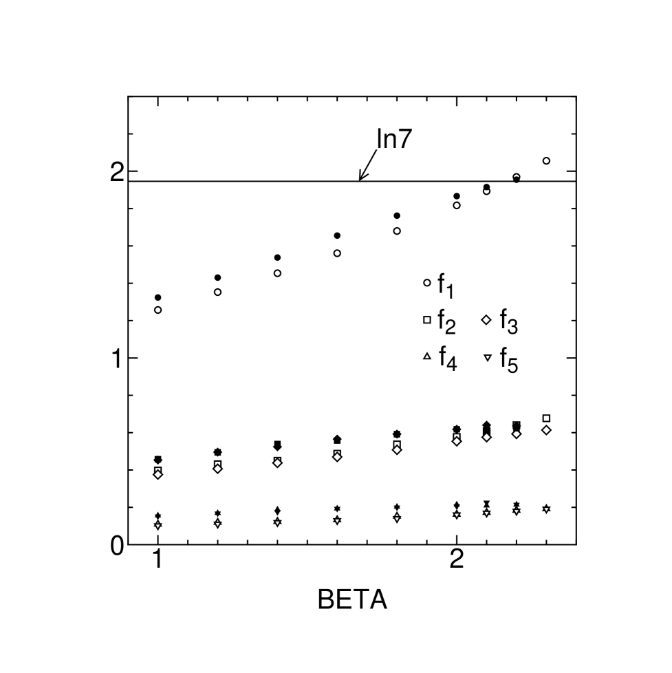
FIG. 2.: Coupling constants $f_{i}$ versus $\beta$ in the strong coupling region. White symbols denote the $SU(2)$ data, whereas black ones show the data of the Wilson form of compact QED with the substitution $\beta_{w}=\beta/2$.

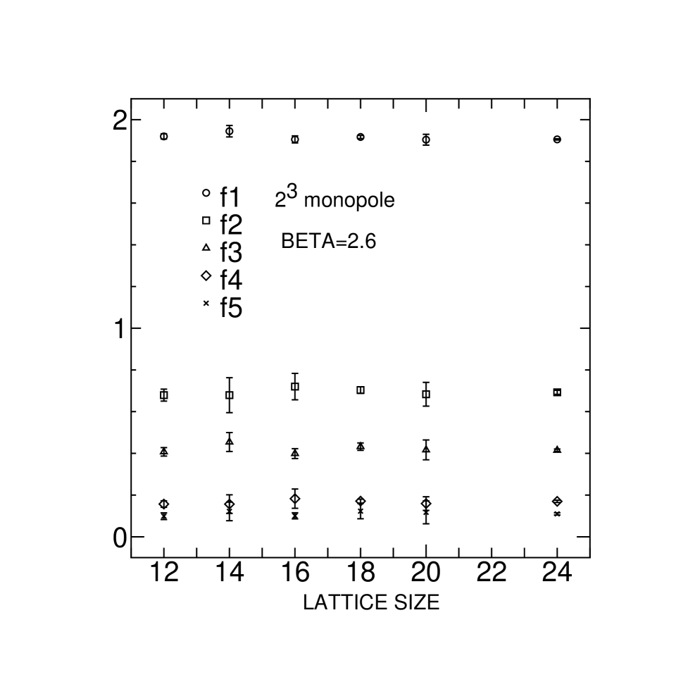
FIG. 3.: Coupling constants $f_{i}$ versus lattice size .

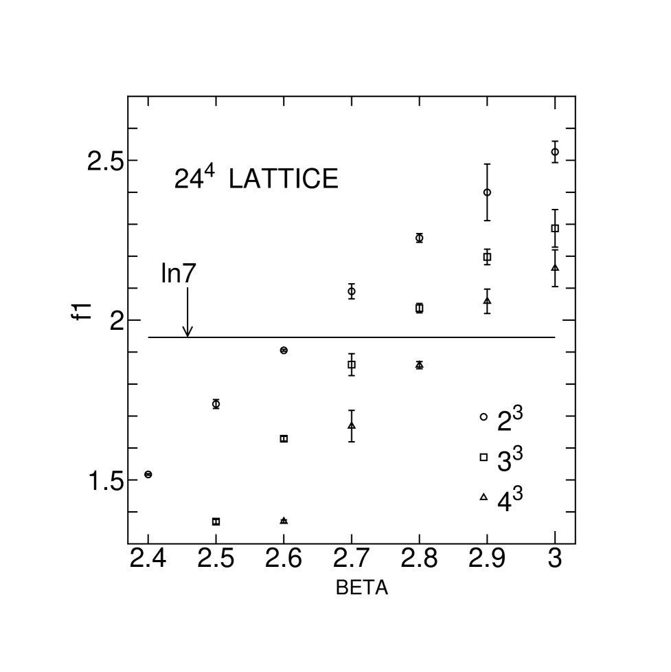
FIG. 4.: Coupling constants $f_{1}$ versus $\beta$ for $2^{3},3^{3}$, and $4^{3}$ extended monopoles on $24^{4}$ lattice.

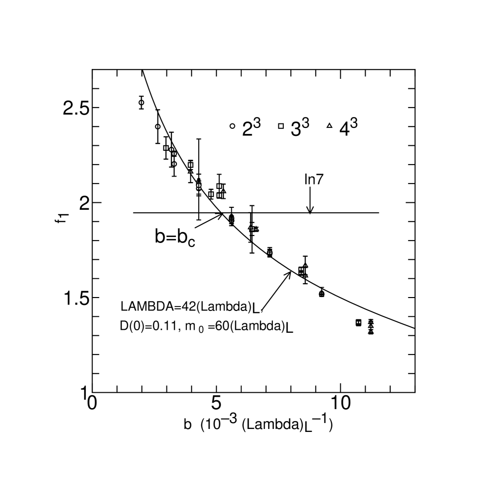
FIG. 5.: Coupling constants $f_{1}$ versus $b$.

FIG. 6.: Coupling constants $f_{2}$ versus $b$. The data with too large errors are omitted.

FIG. 7.: Coupling constants $f_{3}$ versus $b$. The data with too large errors are omitted.

REFERENCES

- [1] G.’tHooft,High Energy Physics, ed.A.Zichichi (Editorice Compositori, Bologna, 1975).
- [2] S. Mandelstam, Phys. Rep. 23C, (1976) 245.
- [3] A.M. Polyakov, Phys. Lett. 59B, (1975) 82.
- [4] T.Banks , Nucl. Phys. B129, (1977) 493.
- [5] T.A. DeGrand and D. Toussaint, Phys. Rev. D22, (1980) 2478.
- [6] G. ’tHooft, Nucl. Phys. B190, (1981) 455.
-
[7]
A.S. Kronfeld , Phys. Lett.
198B, (1987) 516,
A.S. Kronfeld , Nucl.Phys. B293, (1987) 461. - [8] T. Suzuki and I. Yotsuyanagi, Phys. Rev. D42, (1990) 4257; Nucl. Phys. B(Proc. Suppl.) 20, (1991) 236.
- [9] T. Suzuki, Nucl. Phys. B(Proc. Suppl.) 30, (1993) 176 and references therein.
- [10] S. Hioki , Phys. Lett. 272B, (1991) 326.
- [11] H.Shiba and T.Suzuki, Kanazawa University, Report No. Kanazawa 94-07, 1994 to appear in Physics Letters B.
- [12] J.D.Stack, S.D.Neiman and R.J.Wensley, Univ. Illinois, Report No. ILL(TH)-94-#14, 1994.
- [13] M.E. Peshkin, Ann. Phys. 113, (1978) 122.
- [14] J. Frölich and P.A. Marchetti, Euro. Phys. Lett. 2, (1986) 933.
- [15] J. Smit and A.J. van der Sijs, Nucl. Phys. B355, (1991) 603.
- [16] H.Shiba and T.Suzuki, Kanazawa University, Report No. Kanazawa 93-09, 1993.
- [17] H.Shiba and T.Suzuki, Nucl. Phys. B(Proc. Suppl.) 34, (1994) 182.
- [18] R.H. Swendsen,Phys. Rev. Lett. 52, (1984) 1165; Phys. Rev. B30, (1984) 3866, 3875.
- [19] H.Shiba and T.Suzuki, Kanazawa University, Report No. Kanazawa 94-11, 1994.
- [20] T.L. Ivanenko , Phys. Lett. 252B, (1990) 631.
- [21] P. Hasenfratz and F. Niedermayer, Nucl. Phys. B414, (1994) 785.
- [22] E. Kovacs, Phys. Lett. 118B, (1982) 125.
- [23] S. Kitahara, Y. Matsubara and T. Suzuki, in preparation.