CERN-TH.7381/94

PREP N. 1016/94

Supersymmetric corrections to $\epsilon^{\prime}/\epsilon$
at the leading order in QCD and QED

E. Gabrielli

Dip. di Fisica, Università di Roma I “La Sapienza”
P.le A. Moro 2, I-00185 Rome, Italy
INFN – Sezione di Roma I

G.F. Giudice

CERN, Theory Division
CH-1211 Geneva 23, Switzerland

Abstract

We study the corrections to $\epsilon^{\prime}/\epsilon$ in the minimal supersymmetric model at the leading order in QCD and QED. Supersymmetry can increase the standard model prediction for $\epsilon^{\prime}/\epsilon$ by at most 40% for $m_{t}=174$ GeV, an enhancement which is indistinguishable from the present theoretical uncertainties. The most conspicuous effect of supersymmetry is a strong depletion of $\epsilon^{\prime}/\epsilon$. For certain choices of supersymmetric parameters, vanishing and even small negative values of $\epsilon^{\prime}/\epsilon$ can be obtained for the top quark in the CDF range.
CERN-TH.7381/94
PREP. N. 1016/94
July 1994

1 Introduction

CP violation in the kaon system has always been a fertile field in which to test theories beyond the Standard Model (SM). At present the situation for $\epsilon^{\prime}/\epsilon$ is particularly interesting. The experimental results from NA31 at Cern [1]

$$\mbox{Re}~{}\epsilon^{\prime}/\epsilon=23\pm 6.5\times 10^{-4}$$ (1)

and from E731 at Fermilab [2]

$$\mbox{Re}~{}\epsilon^{\prime}/\epsilon=7.4\pm 6.0\times 10^{-4}$$ (2)

are incompatible at the 1-$\sigma$ level. On the theoretical side, there has been great progress in reducing the uncertainties in the prediction for $\epsilon^{\prime}/\epsilon$. The full next-to-leading QCD perturbative corrections have been computed by two groups [3, 4] and developments in lattice calculations should soon provide reliable estimates of the hadronic matrix elements.

Given the inconclusive experimental situation and the notable refinement in the SM calculation for $\epsilon^{\prime}/\epsilon$, the time is right for detailed investigations of $\epsilon^{\prime}/\epsilon$ in theories beyond the SM. If the top quark is indeed as heavy as implied by the CDF measurements [5], the next-to-leading SM prediction for $\epsilon^{\prime}/\epsilon$ sits comfortably in the E731 range, disfavoring the larger NA31 result. While we await improved experimental statistics, which will resolve the conflict between eq. (1) and eq. (2), it is now interesting to see if extensions of the SM can substantially modify the prediction for $\epsilon^{\prime}/\epsilon$ and possibly account for the large value suggested by the NA31 measurement. Furthermore, since the SM prediction for $\epsilon^{\prime}/\epsilon$ suffers a strong accidental cancellation among the different contributions for the top quark in the range of interest, it is conceivable that even modest new-physics effects will easily stand out and sizeably modify the final result.

A notable example of study of $\epsilon^{\prime}/\epsilon$ in theories beyond the SM is contained in ref.[6]. There, in the context of the two-Higgs doublet model, a systematic analysis of $\epsilon^{\prime}/\epsilon$ including leading QCD logarithms has been carried out. It was found that the charged Higgs has the effect of reducing $\epsilon^{\prime}/\epsilon$ with respect to the SM prediction. This reduction occurs partly because of a positive charged-Higgs contribution to $\epsilon$, which suppresses the Cabibbo-Kobayashi-Maskawa (CKM) CP violating parameter $\sin\delta$, and partly because of a new contribution to electroweak penguin and box diagrams, which enhances the degree of cancellation with the strong penguin already present in the SM for a heavy top quark.

The aim of this paper is to generalize the analysis of ref.[6] to the case of the minimal supersymmetric model. Although several analyses of $\epsilon^{\prime}/\epsilon$ in the context of supersymmetry are already present in the literature [7], a complete study including leading QCD logarithms has not been performed. In order to attempt such a study, it is necessary to make precise assumptions regarding the structure of CP violation and flavor-changing neutral currents (FCNC) in the supersymmetric model. Here we choose to work in a minimal version of the model, described in more detail in sect. 2, where both CP violation and FCNC are completely determined by the usual CKM matrix elements. We have several reasons to do this:

i) The corrections to $\epsilon^{\prime}/\epsilon$ considered here are fairly generic to all supersymmetric models. Non-minimal models may contain new CP-violating phases and/or tree-level FCNC, thereby generating extra contributions to $\epsilon^{\prime}/\epsilon$. These contributions are however strongly model-dependent.

ii) The minimal version of the supersymmetric model considered here is very predictive, since CP violation and FCNC are completely determined in terms of only the known CKM angles and phases.

iii) The effective Hamiltonian below the weak scale can be written in terms of the same set of operators used in the case of the SM. This greatly simplifies the analysis, since the anomalous dimension matrix is then completely known at the leading [8] and next-to-leading [9] order. If, for instance, flavor-changing gluino-mediated interactions were included, new operators with different chiral structure would appear and a calculation of new elements of the anomalous-dimension matrix would be required.

Our paper is organized as follows. In sect. 2 we describe the version of the supersymmetric model under investigation and we establish our notation. In sects. 3 and 4 we give the formulae for the supersymmetric corrections to $\epsilon$ and $\epsilon^{\prime}/\epsilon$. The results of our numerical investigation are presented in sect. 5. Finally, in sect. 6 we summarize our results.

2 Supersymmetric model with minimal CP and flavor violation

In general, supersymmetric models have potential sources of new CP violation because of the presence of unremovable phases in the supersymmetry-breaking terms. However, these phases are strongly constrained by measurements on the electric dipole moment of the neutron and must be small, typically less than $10^{-2}-10^{-3}$ [7]. Although there is no compelling theoretical argument which suggests that they are exactly zero, we will make the simplifying (and often used) assumption that the only CP violation resides in the CKM matrix.

It is also well known that FCNC in supersymmetric models can arise at the tree level, since the quark- and squark-mass matrices are diagonalized by different field transformations [10]. Once the heavy supersymmetric particles are integrated out, one is left with FCNC involving ordinary quarks, which are induced by one-loop diagrams with squark and gluino exchange. Their effects are potentially large, since they are O($\alpha_{s}^{2}$), as opposed to the standard model FCNC contributions O($\alpha_{W}^{2}$). The flavor-changing quark-squark-gluino couplings depend however on the details of the supersymmetry-breaking sector, which is still the least-understood part of the theory. It is customary to make the simplifying assumption that all supersymmetry-breaking terms are flavor independent at some grand-unification scale, close to the Planck mass. This is the case if, for instance, the Kähler metric of the underling supergravity theory is flat. In this case flavor-changing quark-squark-gluino couplings are induced by renormalization effects, but their influence in kaon physics is negligible because of the strong limits on gluino and squark masses from hadron colliders [11].

There is growing criticism of this point of view [12], since supergravity theories derived from superstrings do not seem to have flat Kähler metrics and do not seem to have flavor-independent supersymmetry-breaking terms. However, if the supersymmetry-breaking terms have a completely general structure in flavor space, they lead to corrections to $K^{0}-\bar{K}^{0}$ mixing larger than that allowed by experimental constraints. In this case there is need for a suppression of the flavor-changing quark-squark-gluino coupling either by postulating some form of flavor symmetry at the unification scale or by invoking some dynamical mechanism to make squarks more degenerate in mass (e.g. the running from unification to weak scale in a gaugino-dominated supersymmetry-breaking scenario).

In our analysis we will not be concerned about the fundamental mechanism which suppresses FCNC, but we will simply postulate, as we have done for CP violation, that, at the weak scale, FCNC are absent at tree level. As discussed in the introduction, this hypothesis of minimal CP and flavor violation enhances the predictivity of the model and largely simplifies the analysis of QCD effects, since the operator basis of the effective Hamiltonian is the same as in the SM. Let us now briefly present the theoretical framework in which we work, the supersymmetric standard model with minimal CP and flavor violation, and establish our notation.

By making a transformation on superfields, we choose a basis in which the up-quark mass matrix $m_{u}$ is real and diagonal and the down-quark mass matrix is $Vm_{d}$, where $m_{d}$ is real and diagonal and $V$ is the CKM matrix. In this basis, the $6\times 6$ up- and down-squark mass matrices are:

$$\tilde{M}^{2}_{u}=\left(\matrix{\tilde{m}_{u_{L}}^{2}+m_{u}^{2}&A_{u}m_{u}\cr A_{u}m_{u}&\tilde{m}_{u_{R}}^{2}+m_{u}^{2}\cr}\right),$$ (3)

$$\tilde{M}^{2}_{d}=\left(\matrix{\tilde{m}_{d_{L}}^{2}+Vm_{d}^{2}V^{{\dagger}}&A_{d}Vm_{d}\cr A_{d}m_{d}V^{{\dagger}}&\tilde{m}_{d_{R}}^{2}+m_{d}^{2}\cr}\right).$$ (4)

Our minimal CP- and flavor-violation hypothesis states that, at the weak scale, the supersym- metry-breaking terms $\tilde{m}_{u_{L,R}},~{}\tilde{m}_{d_{L,R}}$ and $A_{u,d}$ are CP-conserving and flavor-independent, i.e. real and proportional to the $3\times 3$ identity matrix. If this hypothesis holds, there are no tree-level flavor-violating quark-squark-gluino couplings at the weak scale. Because of the strong constraints imposed by the real part of $K^{0}-\bar{K}^{0}$ mixing, we know that this hypothesis should be approximately satisfied, unless squarks or gluinos are very heavy.

The mass matrices eqs. (3)–(4) can be diagonalized according to

$$T_{u}\tilde{M}^{2}_{u}T^{{\dagger}}_{u}=\mbox{diag}\left(\frac{\tilde{m}_{u_{Li}}^{2}+\tilde{m}_{u_{Ri}}^{2}}{2}+m^{2}_{u_{i}}+\frac{A_{u}m_{u_{i}}}{\sin{2\theta^{u}_{i}}},\frac{\tilde{m}_{u_{Li}}^{2}+\tilde{m}_{u_{Ri}}^{2}}{2}+m^{2}_{u_{i}}-\frac{A_{u}m_{u_{i}}}{\sin{2\theta^{u}_{i}}}\right),$$ (5)

$$T_{d}\tilde{M}^{2}_{d}T^{{\dagger}}_{d}=\mbox{diag}\left(\frac{\tilde{m}_{d_{Li}}^{2}+\tilde{m}_{d_{Ri}}^{2}}{2}+m^{2}_{d_{i}}+\frac{A_{d}m_{d_{i}}}{\sin{2\theta^{d}_{i}}},\frac{\tilde{m}_{d_{Li}}^{2}+\tilde{m}_{d_{Ri}}^{2}}{2}+m^{2}_{d_{i}}-\frac{A_{d}m_{d_{i}}}{\sin{2\theta^{d}_{i}}}\right),$$ (6)

with $i=1,2,3$ and where

$$T_{u}=\left(\matrix{C_{u}&S_{u}\cr-S_{u}&C_{u}\cr}\right),~{}~{}~{}T_{d}=\left(\matrix{C_{d}V^{{\dagger}}&S_{d}\cr-S_{d}V^{{\dagger}}&C_{d}\cr}\right),$$ (7)

$$C_{u,d} = \mbox{diag}\left(\cos{\theta_{i}^{u,d}}\right),~{}~{}~{}~{}~{}S_{u,d}=\mbox{diag}\left(\sin{\theta_{i}^{u,d}}\right),$$ (8)

$$\tan{2\theta_{i}^{u,d}} = \frac{2A_{u,d}m_{i}^{u,d}}{\tilde{m}_{u_{Li},d_{Li}}^{2}-\tilde{m}_{u_{Ri},d_{Ri}}^{2}}.$$ (9)

The chargino mass matrix is diagonalized by two orthogonal $2\times 2$ matrices $U$ and $V$, according to:

$$U\left(\matrix{M&m_{{\scriptscriptstyle W}}\sqrt{2}\sin{\beta}\cr m_{{\scriptscriptstyle W}}\sqrt{2}\cos{\beta}&\mu\cr}\right)V^{-1}=\left(\matrix{\tilde{m}_{\chi_{1}}&0\cr 0&\tilde{m}_{\chi_{2}}\cr}\right),$$

where $\tan{\beta}$ is the ratio of the two Higgs vacuum expectation values, $M$ is the weak gaugino mass, and $\mu$ is the Higgs superfield mixing parameter, taken here to be real.

In order to compute the relevant one-loop diagrams, we need the interaction of charginos $(\tilde{\chi}_{j},~{}j=1,2)$ with down quarks ($d)$ and up squarks $(\tilde{u}_{k},~{}k=1,2)$ in terms of mass eigenstates:

$${\cal L}_{\chi}=g\bar{d}V^{\dagger}\left(Z^{jk}\frac{1-\gamma_{5}}{2}+Y^{jk}\frac{1+\gamma_{5}}{2}\right)\tilde{\chi}_{j}^{(-)}\tilde{u}_{k}+\mbox{h.c.},$$ (10)

$$Z^{jk} = \frac{m_{d}}{\sqrt{2}m_{{\scriptscriptstyle W}}\cos{\beta}}U_{j2}\left(\begin{array}[]{c}\cos{\theta^{u}}\\ -\sin{\theta^{u}}\\ \end{array}\right)_{k}$$ (13)

$$Y^{jk} = \frac{m_{u}}{\sqrt{2}m_{{\scriptscriptstyle W}}\sin{\beta}}V_{j2}\left(\begin{array}[]{c}\sin{\theta^{u}}\\ \cos{\theta^{u}}\\ \end{array}\right)_{k}-V_{j1}\left(\begin{array}[]{c}\cos{\theta^{u}}\\ -\sin{\theta^{u}}\\ \end{array}\right)_{k},$$ (18)

where flavor indices are understood. The CP- and flavor-violation properties of the interaction Lagrangian in eq. (10) are determined by the familiar CKM matrix. This property is satisfied also by the charged-Higgs interactions with quarks:

$${\cal L}_{{\scriptscriptstyle H}}=\frac{g}{\sqrt{2}m_{{\scriptscriptstyle W}}}H^{+}\bar{u}\left(\frac{1}{\tan\beta}m_{u}V\frac{1-\gamma_{5}}{2}+\tan\beta Vm_{d}\frac{1+\gamma_{5}}{2}\right)d+\mbox{h.c.}$$ (19)

We conclude this section by summarizing the free parameters necessary to specify the supersymmetric model, in addition to those of the SM. Whenever convenient, we choose to redefine the original parameters and work with physical particle masses as input. For the first two generations of up-squarks $m_{u}$ is negligible with respect to $\tilde{m}_{u_{L,R}}$ and we will take these squarks to be degenerate in mass, i.e. $\tilde{m}_{u_{L}}\simeq\tilde{m}_{u_{R}}\equiv\tilde{m}$. This is merely a simplifying assumption which will not affect our conclusions. The mixing between the two stops cannot be neglected. We choose as input parameters the lightest stop mass, $m_{\tilde{t}}$, and the stop mixing angle $\theta$ (which can be chosen in the range between 0 and $\pi$, without loss of generality). The mass of the heavier stop ($m_{\tilde{T}}$) is then given by:

$$m_{\tilde{T}}^{2}=2\tilde{m}+2m_{t}^{2}-m_{\tilde{t}}^{2}.$$

The chargino mass matrix is defined by three parameters: we choose them to be the lightest chargino mass ($m_{\chi}$), the ratio of Higgs vacuum expectation values ($\tan{\beta}$), and the weak gaugino mass ($M$). The last free parameter is the charged-Higgs mass ($M_{H^{+}}$), while the relevant $H^{\pm}$ couplings are completely determined once the value of $\tan{\beta}$ is fixed. Therefore the model requires seven input parameters: $\tilde{m},~{}m_{\tilde{t}},~{}\theta,~{}m_{\chi},~{}\tan{\beta},{}~{}M,~{}M_{H^{+}}$. Notice that some of these seven free parameters may become related with one other if additional assumptions are made (specific relations at the GUT scale, constraints from electroweak symmetry breaking, etc.). We prefer to treat them as independent variables in order to describe a larger class of models.

3 The parameter $\epsilon$

The parameter $\epsilon$ gives a measure of the indirect CP-violation in kaon decays. It is defined as

$$\epsilon=\frac{e^{i\pi/4}}{\sqrt{2}\Delta m_{K}}\mbox{Im}M_{12},$$ (20)

where $M_{12}$ is the imaginary part of the off-diagonal element of the neutral kaon system $(K^{0},\bar{K}^{0})$ mass matrix, and $\Delta m_{K}$ is the $K_{L}-K_{S}$ mass difference.

By evaluating the relevant $\Delta S=2$ box diagrams in figure 1a-b, we obtain

$$\epsilon = e^{i\pi/4}\frac{G_{F}^{2}}{12\sqrt{2}\pi^{2}}f^{2}_{{\scriptscriptstyle K}}\frac{m_{{\scriptscriptstyle K}}}{\Delta m_{{\scriptscriptstyle K}}}B_{K}m^{2}_{{\scriptscriptstyle W}}\sum_{i}\left[(\mbox{Im}\lambda_{c}^{2})\eta_{1}^{(i)}S^{(i)}(c,c)+\right.$$ (21)

$$\left.(\mbox{Im}\lambda_{t}^{2})\eta_{2}^{(i)}S^{(i)}(t,t)+2(\mbox{Im}\lambda_{c}\lambda_{t})\eta_{3}^{(i)}S^{(i)}(c,t)\right]$$

where $\lambda_{i}=V_{id}^{*}V_{is}$, $f_{\scriptscriptstyle K}=161$ MeV is the kaon decay constant, and $B_{K}$ is the non-perturbative parameter which defines the normalization of the relevant hadronic matrix element in units of the vacuum-insertion value. The coefficients $\eta_{i}$ include the QCD corrections to the box diagrams and are given in table 1. The values of $\eta_{i}$ for the box diagrams involving squarks and charginos are all equal to the SM value of $\eta_{2}$ because we are assuming that the supersymmetric particles are integrated out at the scale of the $W$ boson.

The functions $S^{(i)}(c,t)$ result from calculation of the box diagrams with exchange of quarks and two W bosons ($WW$), two charged Higgs bosons ($HH$), one W and one charged Higgs ($HW$), and with exchange of squarks and charginos ($\chi$):

$$S^{{\scriptscriptstyle W}{\scriptscriptstyle W}}(c,t) = S(x_{c{\scriptscriptstyle W}},x_{t{\scriptscriptstyle W}})$$

$$S^{{\scriptscriptstyle H}{\scriptscriptstyle H}}(c,t) = \frac{x_{{\scriptscriptstyle H}{\scriptscriptstyle W}}}{4\tan^{4}{\beta}}L_{2}(x_{c{\scriptscriptstyle W}},x_{t{\scriptscriptstyle W}},1)$$

$$S^{{\scriptscriptstyle H}{\scriptscriptstyle W}}(c,t) = \frac{2}{\tan^{2}{\beta}}\left[\frac{1}{4}L_{2}(x_{c{\scriptscriptstyle W}},x_{t{\scriptscriptstyle W}},x_{{\scriptscriptstyle H}{\scriptscriptstyle W}})-L_{1}(x_{c{\scriptscriptstyle W}},x_{t{\scriptscriptstyle W}},x_{{\scriptscriptstyle H}{\scriptscriptstyle W}})\right]$$

$$S^{\chi}(c,t) = f(u,u)-f(u,c)-f(u,t)+f(c,t)$$

$$f(c,t) = \sum_{\stackrel{{\scriptstyle i,j=1,2}}{{\scriptstyle{h,k=1,2}}}}\frac{x_{{\scriptscriptstyle W}\chi_{j}}}{4}Y_{i\tilde{c}_{h}}Y_{i\tilde{t}_{k}}Y_{j\tilde{c}_{h}}Y_{j\tilde{t}_{k}}L_{3}(x_{\tilde{t}_{k}\chi_{j}},x_{\tilde{c}_{h}\chi_{j}},x_{\chi_{i}\chi_{j}}).$$ (22)

We have denoted $x_{ab}\equiv m_{a}^{2}/m_{b}^{2}$ for generic indices $a,b$, and have collected the functions $S$ and $L_{1,2,3}$ in the appendix. The expressions for the charged-Higgs contributions to short-distance effects given in this and the next section agree with ref. [6], and the expressions for the chargino contributions agree with the existent literature whenever results are available (see, in particular, ref.[13]).

For a given set of supersymmetric parameters, one can compare the theoretical prediction for $\epsilon$ in eq. (21) with the experimental result and then determine $\delta$, the CP-violating phase in the “standard” representation [14] of the CKM matrix. In general one obtains two solutions for $\delta$ but, in most of the parameter space, one of them is ruled out by the experimental data on $B^{0}-\bar{B}^{0}$ mixing and on the $b\to s\gamma$ branching ratio.

The $B^{0}-\bar{B}^{0}$ mixing is determined by the box diagrams in figure 1c-d in a manner analogous to $\epsilon$:

$$x_{d}\equiv\frac{\Delta m_{B}}{\Gamma_{B}}=\tau_{B}\frac{G_{F}^{2}}{6\pi^{2}}\eta_{QCD}m_{B}B_{B}f_{B}^{2}m_{{\scriptscriptstyle W}}^{2}|V_{td}|^{2}\sum_{i}S^{(i)}(t,t).$$ (23)

We take $m_{B}=5.28$ GeV, the perturbative QCD correction parameter $\eta_{QCD}=0.84$, and the experimental determination from ARGUS [15] and CLEO [16] for $x_{d}=0.70\pm 0.13.$

The expression for the decay rate of $b\to s\gamma$ in supersymmetry can be found in ref. [13] (or, in a notation very similar to the one employed here, in ref. [17]) and will not be repeated here. In our analysis we will impose the constraint on the inclusive branching ratio $BR(b\to s\gamma)<5.4\times 10^{-4}$ obtained by CLEO [18]. The numerical results will be presented in sect. 5.

4 The parameter $\epsilon^{\prime}$

The parameter $\epsilon^{\prime}$ gives a measure of the direct CP-violation in kaon decays. It is defined as follows:

$$\epsilon^{\prime}=-\frac{\omega}{\sqrt{2}}\xi\left(1-\Omega\right)e^{i\tilde{\phi}},$$ (24)

where

$$\xi=\frac{\mbox{Im}A_{0}}{\mbox{Re}A_{0}},~{}~{}~{}~{}~{}\omega=\frac{\mbox{Re}A_{2}}{\mbox{Re}A_{0}},~{}~{}~{}~{}~{}\Omega=\frac{1}{\omega}\frac{\mbox{Im}A_{2}}{\mbox{Im}A_{0}},~{}~{}~{}~{}~{}\tilde{\phi}=\frac{\pi}{2}+\delta_{2}-\delta_{0}\simeq\frac{\pi}{4}.$$ (25)

$A_{I}$ and $\delta_{I}$ are the amplitudes and final state interaction phases for the decay $K\to(\pi\pi)_{I}$, where $I$ denotes the isospin of the final pion state. Experimentally one has

$$\mbox{Re}A_{0}=3.3\times 10^{-7}\mbox{GeV},~{}~{}~{}~{}~{}~{}~{}~{}\omega\simeq 1/22.$$ (26)

The procedure to relate the amplitudes in eq. (24) to the QCD-improved $\Delta S=1$ effective Hamiltonian is by now standard [19, 21] We will follow the method illustrated in ref. [21], briefly review its results, and show where modifications due to the supersymmetric contributions are necessary.

In the SM, after integrating out the heavy degrees of freedom at the scale of the $W$ boson, the tree-level $\Delta S=1$ Hamiltonian becomes:

$$H_{eff}^{\Delta S=1}=\frac{G_{F}}{\sqrt{2}}V_{ud}V^{*}_{us}\left[\left(1-\tau\right)\left(Q^{u}_{2}-Q^{c}_{2}\right)+\tau\left(Q^{u}_{2}-Q^{t}_{2}\right)\right],$$ (27)

where

$$\tau=-\frac{V_{td}V^{*}_{ts}}{V_{ud}V^{*}_{us}},~{}~{}~{}~{}~{}Q_{2}^{q}=\left(\bar{s}q\right)_{V-A}\left(\bar{q}d\right)_{V-A},~{}~{}q=u,c,t.$$ (28)

With QCD corrections taken into account, the effective Hamiltonian at an energy scale $\mu$ below the charm mass is obtained by replacing in eq. (27) the operators $Q_{2}^{q}$ with the renormalized four-fermion operators $Q_{i}(\mu)$ as follows:

$$\left(Q_{2}^{u}-Q_{2}^{c}\right)\rightarrow\sum_{i=1}^{10}z_{i}(\mu)Q_{i}(\mu),~{}~{}~{}~{}~{}~{}~{}~{}\left(Q_{2}^{u}-Q_{2}^{t}\right)\rightarrow\sum_{i=1}^{10}v_{i}(\mu)Q_{i}(\mu).$$ (29)

In eq. (29), $v_{i}(\mu)$ and $z_{i}(\mu)$ correspond to the relevant Wilson coefficients and the complete basis used for the operators $Q_{i}$ is

$$Q_{1} = (\bar{s}d)_{V-A}(\bar{u}u)_{V-A},{}~{}~{}~{}~{}~{}~{}~{}~{}~{}~{}~{}~{}~{}~{}Q_{2}~{}=~{}(\bar{s}u)_{V-A}(\bar{u}d)_{V-A},$$

$$Q_{3} = (\bar{s}d)_{V-A}\sum_{q=u,d,s}(\bar{q}q)_{V-A},{}~{}~{}~{}~{}~{}~{}~{}~{}~{}Q_{4}~{}=~{}\sum_{q=u,d,s}(\bar{s}q)_{V-A}(\bar{q}d)_{V-A},$$

$$Q_{5} = (\bar{s}d)_{V-A}\sum_{q=u,d,s}(\bar{q}q)_{V+A},{}~{}~{}~{}~{}~{}~{}~{}~{}~{}Q_{6}~{}=~{}-8\sum_{q=u,d,s}(\bar{s}_{L}q_{R})(\bar{q}_{R}d_{L}),$$

$$Q_{7} = \frac{3}{2}(\bar{s}d)_{V-A}\sum_{q=u,d,s}e_{q}(\bar{q}q)_{V+A},{}~{}~{}~{}~{}~{}Q_{8}~{}=~{}-12\sum_{q=u,d,s}e_{q}(\bar{s}_{L}q_{R})(\bar{q}_{R}d_{L}),$$

$$Q_{9} = \frac{3}{2}(\bar{s}d)_{V-A}\sum_{q=u,d,s}e_{q}(\bar{q}q)_{V-A},{}~{}~{}~{}~{}Q_{10}~{}=~{}\frac{3}{2}\sum_{q=u,d,s}e_{q}(\bar{s}q)_{V-A}(\bar{q}d)_{V-A},$$ (30)

where $e_{q}$ is the electric charge of the quark $q$, $(V\pm A)$ refer to $\gamma_{\mu}(1\pm\gamma_{5})$, and $q_{L,R}=1/2(1\pm\gamma_{5})q$. We neglect here magnetic-moment operators [22], since their contribution is unimportant for our purposes.

In general we can therefore write the effective $\Delta S=1$ Hamiltonian at the scale $\mu$ as

$$H_{eff}^{\Delta S=1}=\frac{G_{F}}{\sqrt{2}}V_{ud}V^{*}_{us}\sum_{i=1}^{10}C_{i}(\mu)Q_{i}(\mu),$$ (31)

where

$$C_{i}(\mu)=z_{i}(\mu)+\tau y_{i}(\mu);~{}~{}~{}~{}~{}y_{i}(\mu)\equiv v_{i}(\mu)-z_{i}(\mu).$$ (32)

The Wilson coefficients $C_{i}$ are chosen to match the short-distance contribution at the appropriate scale where heavy particles are integrated out, and then evolved using the renormalization group equation:

$$\left[\mu\frac{\partial}{\partial\mu}+\beta(g)\frac{\partial}{\partial g}-\hat{\gamma}^{T}(g^{2},\alpha)\right]\vec{C}\left(\frac{m_{{\scriptscriptstyle W}}^{2}}{\mu^{2}},g^{2},\alpha\right)=0,$$ (33)

where $\vec{C}$ stands for a ten-dimensional vector, $\beta(g)$ is the QCD beta function, and $\alpha$ is the electromagnetic coupling constant (the running of $\alpha$ is neglected). In this paper we use the anomalous-dimension matrix $\hat{\gamma}^{T}(g^{2},\alpha)$ at the leading order in QCD and QED as given in ref. [21], although it is now known at the next-to-leading order [9]. This is perfectly adequate, in view of the large intrinsic uncertainty due to the ignorance of the supersymmetric parameters and to the inescapable model-dependence. Our aim here is just to illustrate the trend of the supersymmetric corrections to $\epsilon^{\prime}/\epsilon$.

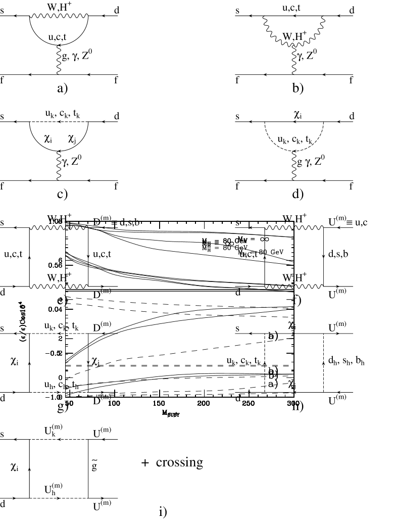
Figure 2: The penguin (a-d) and the box (e-i) diagrams for $\epsilon^{\prime}/\epsilon$ in the minimal supersymmetric SM.

The modifications caused by supersymmetry appear only in the boundary conditions of the Wilson coefficients, which are computed through the appropriate one-loop Feynman diagrams in figure 2. In our analysis we will impose the boundary conditions at the scale $\mu=m_{{\scriptscriptstyle W}}$, although strictly speaking they should apply to the energy scale at which the heavy particles are integrated out. The threshold corrections, originating from this mismatch of energy scales and certainly present in any realistic theory with a non-degenerate mass-spectrum, are numerically not very significant, since the running of $\alpha_{s}$ in the region above $m_{{\scriptscriptstyle W}}$ is not very steep. In the HV renormalization scheme, the boundary conditions for the Wilson coefficients in the minimal supersymmetric model are given by:

$$v_{1}(m_{{\scriptscriptstyle W}}) = \frac{\alpha_{s}({m_{{\scriptscriptstyle W}}})}{16\pi}\left(14-B_{\tilde{g}}\right)$$

$$v_{2}(m_{{\scriptscriptstyle W}}) = 1$$

$$v_{3}(m_{{\scriptscriptstyle W}}) = \frac{\alpha}{6\pi}\frac{1}{\sin^{2}{\theta_{{\scriptscriptstyle W}}}}\left(B^{(d)}+\frac{B^{(u)}}{2}+C\right)-\frac{\alpha_{s}({m_{{\scriptscriptstyle W}}})}{24\pi}E$$

$$v_{4}(m_{{\scriptscriptstyle W}}) = \frac{\alpha_{s}({m_{{\scriptscriptstyle W}}})}{8\pi}E$$

$$v_{5}(m_{{\scriptscriptstyle W}}) = -\frac{\alpha_{s}({m_{{\scriptscriptstyle W}}})}{24\pi}E$$

$$v_{6}(m_{{\scriptscriptstyle W}}) = \frac{\alpha_{s}({m_{{\scriptscriptstyle W}}})}{8\pi}E$$

$$v_{7}(m_{{\scriptscriptstyle W}}) = \frac{\alpha}{6\pi}\left(4C+D\right)$$

$$v_{8}(m_{{\scriptscriptstyle W}}) = 0$$

$$v_{9}(m_{{\scriptscriptstyle W}}) = \frac{\alpha}{6\pi}\left[4C+D+\frac{1}{\sin^{2}{\theta_{{\scriptscriptstyle W}}}}\left(-B^{(d)}+B^{(u)}-4C\right)\right]$$

$$v_{10}(m_{{\scriptscriptstyle W}}) = 0$$ (34)

and

$$z_{1}(m_{{\scriptscriptstyle W}})=v_{1}(m_{{\scriptscriptstyle W}}),~{}~{}z_{2}(m_{{\scriptscriptstyle W}})=v_{2}(m_{{\scriptscriptstyle W}}),~{}~{}z_{i}(m_{{\scriptscriptstyle W}})=0,~{}~{}i=3,10.$$ (35)

The functions which include the contributions from photon-penguins ($D$), Z-penguins ($C$), gluon-penguins ($E$), boxes with external down quarks ($B^{(d)}$) and up quarks ($B^{(u)}$), and gluino-mediated boxes ($B^{({\tilde{g}})}$) are given by:

$$D=D_{SM}(x_{t{\scriptscriptstyle W}})+\frac{1}{\tan^{2}\beta}D_{H}(x_{t{\scriptscriptstyle H}})+\sum_{\stackrel{{\scriptstyle j=1,2}}{{\scriptstyle{k=1,2}}}}\left[Y^{2}_{j\tilde{t}_{k}}x_{{\scriptscriptstyle W}\tilde{t}_{k}}D_{\chi}(x_{\chi_{j}\tilde{t}_{k}})-\left(\tilde{t}\rightarrow\tilde{c}\right)\right]$$ (36)

$$C = C_{SM}(x_{t{\scriptscriptstyle W}})+\frac{x_{t{\scriptscriptstyle W}}}{\tan^{2}\beta}C_{H}(x_{t{\scriptscriptstyle H}})+\sum_{\stackrel{{\scriptstyle i,j=1,2}}{{\scriptstyle{h,k=1,2}}}}\left[Y_{j\tilde{t}_{k}}Y_{i\tilde{t}_{h}}\left\{\frac{1}{2}\delta_{ij}\Delta_{hk}C_{\chi}^{(1)}(x_{\tilde{t}_{h}\chi_{j}},x_{\tilde{t}_{k}\chi_{j}})\right.\right.$$ (37)

$$+ \left.\left.\delta_{hk}\left[U_{i1}U_{j1}C^{(2)}_{\chi}(x_{\chi_{j}\tilde{t}_{k}},x_{\chi_{i}\tilde{t}_{k}})+V_{i1}V_{j1}\left(\frac{1}{16}\log{m^{2}_{\tilde{t}_{k}}}-C^{(1)}_{\chi}(x_{\chi_{j}\tilde{t}_{k}},x_{\chi_{i}\tilde{t}_{k}})\right)\right]\right\}\right.$$

$$- \left.\left(\tilde{t}\rightarrow\tilde{c}\right)\right]$$

$$E=E_{SM}(x_{t{\scriptscriptstyle W}})+\frac{1}{\tan^{2}\beta}E_{H}(x_{t{\scriptscriptstyle H}})+\sum_{\stackrel{{\scriptstyle j=1,2}}{{\scriptstyle{k=1,2}}}}\left[Y^{2}_{j\tilde{t}_{k}}x_{{\scriptscriptstyle W}\tilde{t}_{k}}E_{\chi}(x_{\chi_{j}\tilde{t}_{k}})-\left(\tilde{t}\rightarrow\tilde{c}\right)\right]$$ (38)

$$B^{(d)} = -2B_{SM}(x_{t{\scriptscriptstyle W}})+\frac{1}{8}\sum_{\stackrel{{\scriptstyle i,j=1,2}}{{\scriptstyle{h,k=1,2}}}}Y_{j\tilde{u}_{h}}Y_{i\tilde{u}_{h}}x_{{\scriptscriptstyle W}\chi_{j}}\left[Y_{j\tilde{t}_{k}}Y_{i\tilde{t}_{k}}B_{\chi}^{(d)}(x_{\tilde{t}_{k}\chi_{j}},x_{\tilde{u}_{h}\chi_{j}},x_{\chi_{i}\chi_{j}})\right.$$ (39)

$$- \left.\left(\tilde{t}\rightarrow\tilde{c}\right)\right]$$

$$B^{(u)} = 8B_{SM}(x_{t{\scriptscriptstyle W}})+\frac{1}{4}\sum_{\stackrel{{\scriptstyle i,j=1,2}}{{\scriptstyle{h,k=1,2}}}}U_{j1}U_{i1}x_{{\scriptscriptstyle W}\chi_{j}}\sqrt{x_{\chi_{i}\chi_{j}}}\left[Y_{j\tilde{t}_{k}}Y_{i\tilde{t}_{k}}B_{\chi}^{(u)}(x_{\tilde{t}_{k}\chi_{j}},x_{\tilde{d}_{h}\chi_{j}},x_{\chi_{i}\chi_{j}})\right.$$ (40)

$$- \left.\left(\tilde{t}\rightarrow\tilde{c}\right)\right]$$

$$B^{({\tilde{g}})} = \sum_{\stackrel{{\scriptstyle i=1,2}}{{\scriptstyle{h,k=1,2}}}}\Delta_{hk}x_{{\scriptscriptstyle W}g}\left[\left(V_{i1}^{2}+U_{i1}^{2}\right)B_{\chi}^{(d)}(x_{\chi_{i}g},x_{\tilde{u}_{k}g},x_{\tilde{u}_{h}g})\right.$$ (41)

$$+ \left.2\frac{m_{\chi_{i}}}{m_{g}}V_{i1}U_{i1}B_{\chi}^{(u)}(x_{\chi_{i}g},x_{\tilde{u}_{k}g},x_{\tilde{u}_{h}g})\right],$$

where $\Delta_{hk}=1$ for $h=k$ and $\Delta_{hk}=-1$ for $h\neq k$. Finally, the explicit form of the functions resulting from loop integration is given in the appendix.

Notice that the supersymmetric box diagrams contribute to the operators $Q_{3}$ and $Q_{9}$ via two different functions $B^{(u)}$ and $B^{(d)}$, as opposed to the SM case where a single function ($B_{SM}$) appears. The function $B^{({\tilde{g}})}$ accounts for the contribution of the box diagrams with a gluino, a chargino, and two squarks as internal lines. These diagrams exist also in the limit of flavor-conserving gluino vertices, in which we are working. In order not to further increase the number of free parameters, we have chosen to relate the gluino mass ($m_{\tilde{g}}$) to the $M$ parameter defined in sect. 2 through the GUT relation:

$$m_{\tilde{g}}=\frac{\alpha_{s}(m_{{\scriptscriptstyle W}})\sin{\theta_{{\scriptscriptstyle W}}}M}{\alpha(m_{{\scriptscriptstyle W}})}.$$ (42)

This assumption is however inessential, because the gluino-box contribution to $\epsilon^{\prime}/\epsilon$ is completely negligible.

Using the effective Hamiltonian $H_{eff}^{\Delta S=1}$ of eq. (31), we recast eq. (24) in the form

$$\frac{\epsilon^{\prime}}{\epsilon}=\mbox{Im}\lambda_{t}\frac{G_{F}~{}\omega}{2|\epsilon|\mbox{Re}A_{0}}y_{6}(\mu)\left\langle Q_{6}(\mu)\right\rangle_{0}\Bigl{(}1-\Omega\Bigr{)}$$ (43)

$$\Omega\equiv\Omega_{\eta+\eta^{\prime}}-\sum_{\stackrel{{\scriptstyle i=1,10}}{{i\neq 6}}}\frac{y_{i}(\mu)\left\langle Q_{i}(\mu)\right\rangle_{0}}{y_{6}(\mu)\left\langle Q_{6}(\mu)\right\rangle_{0}}+\frac{1}{\omega}\sum_{i=1,10}\frac{y_{i}(\mu)\left\langle Q_{i}(\mu)\right\rangle_{2}}{y_{6}(\mu)\left\langle Q_{6}(\mu)\right\rangle_{0}},$$ (44)

where $\Omega_{\eta+\eta^{\prime}}$ is the contribution from $\pi-\eta-\eta^{\prime}$ mixing, here taken to be $\Omega_{\eta+\eta^{\prime}}=0.25\pm 0.05$. Following a general convention, we have factored out the dominant contribution from the operator $Q_{6}$ and call $\Omega$ the correction due to the other operators.

In our numerical analysis, we set the renormalization scale $\mu$ at 1 GeV. In order to evaluate eq. (43), we need the relevant hadronic matrix elements at that scale:

$$\left\langle Q_{i}\right\rangle_{I}\equiv\left\langle(\pi\pi)_{I}|Q_{i}|K\right\rangle~{}~{}~{}~{}~{}~{}~{}~{}I=0,2,$$ (45)

where $I$ is the total isospin of the final pion-pion state. In the future, lattice calculations should provide the most reliable evaluation of hadronic matrix elements. For the moment we prefer to follow the approach of ref. [3].

The strategy is to compute the matrix elements $\left\langle Q_{i}\right\rangle_{I}$ at the $m_{c}$ scale and then, using the QCD evolution, to obtain the matrix elements at the scale $\mu<m_{c}$. The advantages of this method are explained in detail in ref. [3]. Starting at $\mu=m_{c}$ one finds [3]:

$$\left\langle Q_{1}\right\rangle_{0} = -\frac{1}{9}XB_{1}^{(1/2)},~{}~{}~{}\left\langle Q_{2}\right\rangle_{0}~{}=~{}\frac{5}{9}XB_{2}^{(1/2)},~{}~{}~{}\left\langle Q_{3}\right\rangle_{0}~{}=~{}\frac{1}{3}XB_{3}^{(1/2)},$$

$$\left\langle Q_{4}\right\rangle_{0} = \left\langle Q_{3}\right\rangle_{0}+\left\langle Q_{2}\right\rangle_{0}-\left\langle Q_{1}\right\rangle_{0},~{}~{}~{}\left\langle Q_{5}\right\rangle_{0}~{}=~{}\frac{1}{3}B_{5}^{(1/2)}\left\langle\overline{Q_{6}}\right\rangle_{0},$$

$$\left\langle Q_{6}\right\rangle_{0} = -4\sqrt{\frac{3}{2}}\left[\frac{m_{{\scriptscriptstyle K}}^{2}}{m_{s}(\mu)+m_{d}(\mu)}\right]^{2}\frac{f_{\pi}}{k}B_{6}^{(1/2)},$$

$$\left\langle Q_{7}\right\rangle_{0} = -\left[\frac{1}{6}\left\langle\overline{Q_{6}}\right\rangle_{0}(k+1)-\frac{X}{2}\right]B_{7}^{(1/2)},$$

$$\left\langle Q_{8}\right\rangle_{0} = -\left[\frac{1}{2}\left\langle\overline{Q_{6}}\right\rangle_{0}(k+1)-\frac{X}{6}\right]B_{8}^{(1/2)},$$

$$\left\langle Q_{9}\right\rangle_{0} = \frac{3}{2}\left\langle Q_{1}\right\rangle_{0}-\frac{1}{2}\left\langle Q_{3}\right\rangle_{0},~{}~{}\left\langle Q_{10}\right\rangle_{0}~{}=~{}\left\langle Q_{2}\right\rangle_{0}+\frac{1}{2}\left\langle Q_{1}\right\rangle_{0}-\frac{1}{2}\left\langle Q_{3}\right\rangle_{0},$$ (46)

$$\left\langle Q_{1}\right\rangle_{2} = \left\langle Q_{2}\right\rangle_{2}=\frac{4\sqrt{2}}{9}XB_{1}^{(3/2)},~{}~{}~{}\left\langle Q_{i}\right\rangle_{2}~{}=~{}0~{}~{}~{}~{}~{}~{}~{}i=3,...,6,$$

$$\left\langle Q_{7}\right\rangle_{2} = -\left[\frac{k}{6\sqrt{2}}\left\langle\overline{Q_{6}}\right\rangle_{0}+\frac{X}{\sqrt{2}}\right]B_{7}^{(3/2)},$$

$$\left\langle Q_{8}\right\rangle_{2} = -\left[\frac{k}{2\sqrt{2}}\left\langle\overline{Q_{6}}\right\rangle_{0}+\frac{\sqrt{2}}{6}X\right]B_{8}^{(3/2)},$$

$$\left\langle Q_{9}\right\rangle_{2} = \left\langle Q_{10}\right\rangle_{2}=\frac{3}{2}\left\langle Q_{1}\right\rangle_{2},$$ (47)

where

$$k = \frac{\Lambda_{\chi}^{2}}{m_{{\scriptscriptstyle K}}^{2}-m_{\pi}^{2}}\simeq 4.55$$

$$X = \sqrt{\frac{3}{2}}f_{\pi}\left(m_{{\scriptscriptstyle K}}^{2}-m_{\pi}^{2}\right)=3.71\times 10^{-2}\mbox{GeV}^{3}$$

$$\left\langle\overline{Q_{6}}\right\rangle_{0} = \frac{\left\langle Q_{6}\right\rangle_{0}}{B_{6}^{(1/2)}}$$ (48)

and $B_{i}^{(1/2)}$, $B_{i}^{(3/2)}$ stand respectively for the $\Delta I=1/2,~{}3/2$ transitions.

These matrix elements are obtained using the vacuum-insertion approximation and soft-pion theorems, with all of the non-perturbative information included in the $B_{i}$ parameters. We will use the following values at the scale $\mu=m_{c}$ [3]:

$$B_{1}^{(1/2)}=5.2,~{}~{}B_{2}^{(1/2)}=5.8\pm 1.1,~{}~{}B_{6}^{(1/2)}=1\pm 0.2,$$

$$B_{1}^{(3/2)}=0.55,~{}~{}B_{8}^{(3/2)}=1\pm 0.2.$$ (49)

The remaining $B_{i}$ parameters play only a minor role in the analysis of $\epsilon^{\prime}/\epsilon$ and we will set them equal to 1.

5 Results

It is well known [20, 21], [3, 4] that the SM value of $\epsilon^{\prime}/\epsilon$ is typically of order $10^{-4}$ for $m_{t}=150-190$ GeV, decreases for increasing $m_{t}$, and becomes zero for $m_{t}=200-220$ GeV. This accidental cancellation occurs because the parameter $\Omega$ in eq. (43) approaches 1 as the top quark mass reaches these large values.

There are two main sources of uncertainty in the SM prediction for $\epsilon^{\prime}/\epsilon$. One affects the Wilson coefficients and comes from uncertainties in SM parameters such as the CKM angles, $m_{t}$, $m_{s}$, and $\Lambda_{QCD}$. As measurements on these parameters become more precise, the calculations of the Wilson coefficients stand on firmer ground. We summarize in table 2 the SM parameter values (and their relative errors) chosen for our numerical analysis.

The second source of uncertainty stems from the hadronic matrix elements, i.e. from the $B_{i}$ parameters discussed in sect. 4. At present lattice calculations seem to be the only tool capable of significantly reducing errors.

Our goal in this paper is to study the effect of supersymmetry on $\epsilon^{\prime}/\epsilon$. Because of the cancellation mentioned above, the SM value of $\epsilon^{\prime}/\epsilon$ is typically smaller than its separate contributions. In this situation, new-physics effects have the chance to emerge and increase significantly the total result.

In our analysis we will vary in the experimentally-allowed region the seven free parameters of the minimal supersymmetric model defined in sect. 2. The parameters are subject to the constraints that all charged supersymmetric particle masses be heavier than $m_{Z}/2$ and that the common squark mass satisfy the CDF bound $\tilde{m}>126$ GeV [11]. We also use the tree-level mass bound $M_{H^{+}}>m_{{\scriptscriptstyle W}}$ obeyed by the supersymmetric charged Higgs boson and the bound $\tan\beta>1$ implied by radiative electroweak symmetry breaking.

Since we are interested here in studying the trend of the supersymmetric corrections, we start by fixing the SM input parameters to the central values given in table 2. As can be seen from eq. (43), there are three sources of new-physics corrections to $\epsilon^{\prime}/\epsilon$: the CKM phase ($\mbox{Im}\lambda_{t}$), the strong penguin ($y_{6}$), and the rest of the electroweak contribution ($\Omega$). Let us first consider the CKM phase $\delta$, which is determined by the $\epsilon$ parameter, eq. (21).

By scanning over the supersymmetric parameter space, we obtain the allowed region of $\delta$ shown as a function of $m_{\mbox{susy}}$ in fig. 3a (for $M_{H^{+}}=80$ GeV) and in fig. 3b (for $M_{H^{+}}=\infty$), for $m_{t}=174$ GeV. We have defined $m_{\mbox{susy}}$ as the mass of the lightest charged supersymmetric particle (either the chargino or the stop). With this definition, it is easy to see from fig. 3 how improvements on the experimental limits on supersymmetric particle masses (e.g. from LEP 200) will affect the allowed range of $\delta$. The two SM solutions for $\cos\delta$ correspond to the minimum values allowed by the supersymmetric bands in fig. 3b. In other words, the presence of supersymmetry has the effect of reducing the value of $\sin\delta$, both for the solution in the first quadrant ($\cos\delta>0$) and in the second quadrant ($\cos\delta<0$); the lighter the charged Higgs, the stronger the reduction. Since $\epsilon^{\prime}/\epsilon$ is proportional to $\sin\delta$, this has the effect of decreasing $\epsilon^{\prime}/\epsilon$, as discussed below. If the constraints from $B^{0}-\bar{B}^{0}$ mixing and $b\to s\gamma$ are imposed, only the solution in the first quadrant survives, as shown in fig. 4. This is true only because we have fixed the SM parameters at their central values. If all uncertainties are properly taken into account, some solutions for $\delta$ in the second quadrant can still be found. In general however a heavy top disfavors solutions with $\cos\delta<0$, unless $f_{B}$ is small.

The impact of supersymmetry on the prediction for $\epsilon^{\prime}/\epsilon$ is illustrated in fig. 5. This shows the allowed range of $\epsilon^{\prime}/\epsilon$ as a function of $m_{\mbox{susy}}$ for $M_{H^{+}}=80$ GeV (fig. 5a) and $M_{H^{+}}=\infty$ (fig. 5b) with $m_{t}=174$ GeV and with the parameters subject to the constraints from $B^{0}-\bar{B}^{0}$ mixing and $b\to s\gamma$. In fig. 5a the strong reduction of $\epsilon^{\prime}/\epsilon$ in the presence of a relatively light charged Higgs is apparent. This is partly caused by the decrease in $\sin\delta$ mentioned above. However the main reason for such small values of $\epsilon^{\prime}/\epsilon$ is that $\Omega$ can approach 1, allowing a complete cancellation for values of $m_{t}$ smaller than that found in the SM. As shown in fig. 5a, $\epsilon^{\prime}/\epsilon$ can even reach negative values if $M_{H^{+}}$ is small enough. The charged-Higgs effect on $\epsilon^{\prime}/\epsilon$ has already been studied by the authors of ref.[6] and we confirm here their results.

As discussed above, the chargino contribution has always the effect to lower $\sin\delta$. However, depending on the choice of the supersymmetric parameters, the chargino contribution to $\Omega$ can have either sign. As a consequence, $\epsilon^{\prime}/\epsilon$ in supersymmetry can also be enhanced with respect to the SM value, as seen in fig. 5. This enhancement is numerically rather small, at most 40%. For comparison, the SM value of $\epsilon^{\prime}/\epsilon$, which can be read in fig. 5b in the limit $m_{\mbox{susy}}\to\infty$, corresponds to the leading-order calculation. We recall that next-to-leading effects tend to suppress even further the value of $\epsilon^{\prime}/\epsilon$ [3, 4].

In tables 3 and 4 we report the values of the three different contributions $\sin\delta$, $\Omega$, and $y_{6}\left\langle Q_{6}\right\rangle_{0}$ corresponding to the minimum and maximum values of $\epsilon^{\prime}/\epsilon$. Notice that the main effect of supersymmetry resides in $\sin\delta$ and $\Omega$, while $y_{6}\left\langle Q_{6}\right\rangle_{0}$ is never reduced by more than 5%. Finally fig. 6 shows how the prediction for $\epsilon^{\prime}/\epsilon$ is affected as the constraints from $B^{0}-\bar{B}^{0}$ mixing and $b\to s\gamma$ are removed.

It is interesting to know for which values of the supersymmetric parameters $\epsilon^{\prime}/\epsilon$ reaches its minimum and maximum. The charged-Higgs contribution is maximized for the minimum allowed values of $M_{H^{+}}$ and $\tan\beta$, respectively equal to $m_{\scriptscriptstyle W}$ and 1. Notice that all charged-Higgs contributions are proportional to $1/\tan^{2}\beta$ and therefore rapidly decrease as $\tan\beta$ increases. The chargino contribution is typically maximized when the chargino and the lightest stop masses are small (i.e. of the order of $m_{\mbox{susy}}$) and $\tilde{m}\to\infty$. In this limit, flavor symmetry is indeed maximally broken. Also the chargino contribution minimizes $\epsilon^{\prime}/\epsilon$ for $\tan\beta=1$ and maximizes it for $\tan\beta$ in the range 3-5.

Next we want to take into account the experimental and theoretical errors of the SM input parameters. We have used the following approach. We first fix the SM parameters to their central values and, for given $m_{\mbox{susy}}$ and $M_{H^{+}}$, we compute the supersymmetric parameters which respectively minimize and maximize the contribution to $\epsilon^{\prime}/\epsilon$. Then, keeping these values of the supersymmetric parameters fixed, we generate a large number of configurations using gaussian and flat distributions for the SM inputs with respectively experimental and theoretical errors. We obtain an event distribution for $\epsilon^{\prime}/\epsilon$, from which we can compute the average value and standard deviation. Notice that by following this procedure we are averaging over solutions with positive and negative $\cos\delta$, both of which are allowed when the uncertainties on the SM inputs are taken into account.

The results are shown in tables 5–7, for three values of the top quark mass, $m_{t}=150,~{}174,~{}190$ GeV, imposing the constraints from $B^{0}-\bar{B}^{0}$ mixing and $b\to s\gamma$. The effect of relaxing these constraints is illustrated in table 8. We observe that the enhancement of $\epsilon^{\prime}/\epsilon$ in supersymmetry is indistinguishable from the SM result within a standard deviation, even in the most favorable case $m_{t}=190$ GeV. On the other hand, the depletion of $\epsilon^{\prime}/\epsilon$ is substantial and statistically significant. Unfortunately the experimental sensitivity is presently not sufficient to identify such small values of $\epsilon^{\prime}/\epsilon$.

6 Conclusions

We have studied the corrections to $\epsilon^{\prime}/\epsilon$ in the supersymmetric model with minimal CP and flavor violation at the leading order in QCD and QED. Our results are the following.

Supersymmetry can enhance the SM prediction for $\epsilon^{\prime}/\epsilon$ by at most 40% for $m_{t}=174$ GeV and up to 60% for $m_{t}=190$ GeV. This enhancement is of the same order of magnitude as the SM prediction within one standard deviation and therefore it is not experimentally distinguishable. In this respect, minimal supersymmetry cannot explain a value of $\epsilon^{\prime}/\epsilon$ as large as the one suggested by the NA31 measurement [1]. The enhancement is caused by a reduction of the electroweak factor $\Omega$ and it is attained for chargino and stop masses just beyond the LEP limit, with all the other squarks and the charged Higgs considerably heavier.

The most conspicuous effect of minimal supersymmetry is however a strong depletion of $\epsilon^{\prime}/\epsilon$. For certain choices of supersymmetric parameters, vanishing and even small negative values of $\epsilon^{\prime}/\epsilon$ can be obtained for the top quark in the CDF range [5], $m_{t}=150-190$ GeV. Unfortunately sensitivity to values of $\epsilon^{\prime}/\epsilon$ below $10^{-4}$ represents experimentally a very challenging proposition. This depletion is caused by a reduction of the value of $\sin\delta$ extracted from $\epsilon$ and by an increase in the electroweak correction $\Omega$, which can become equal to 1 or larger. From the short-distance point of view, the dominant corrections at the origin of the $\epsilon^{\prime}/\epsilon$ depletion come from a light charged Higgs, and from charginos and stops just beyond the LEP limit.

Acknowledgement

One of the authors, E.G. , would like to thank S. Ambrosanio, M. Ciuchini, and E. Franco for useful discussions and the Theoretical Physics Division of CERN for its kind hospitality.

Appendix A

In this appendix we give the expressions for the functions which enter the penguin and box diagrams.

Box($\Delta$ S=2 )

$$S(x,y) = xy\left\{\left[\frac{1}{4}+\frac{3}{2}\frac{1}{1-x}-\frac{3}{4}\frac{1}{(1-x)^{2}}\right]\frac{\log x}{x-y}+\left(x\leftrightarrow y\right)-\frac{3}{4}\frac{1}{(1-x)(1-y)}\right\}$$

$$L_{1}(x,y,z) = xy\left[F(x,y,z)+F(y,z,x)+F(z,x,y)\right]$$

$$L_{2}(x,y,z) = xy\left[xF(x,y,z)+yF(y,z,x)+zF(z,x,y)\right]$$

$$L_{3}(x,y,z) = \frac{1}{xy}L_{2}(x,y,z)$$

$$F(x,y,z) = \frac{x\log{x}}{(x-1)(x-y)(x-z)}$$

Box($\Delta$ S=1)

$$B_{SM}(x) = -\frac{x}{4(x-1)}+\frac{x}{4(x-1)^{2}}\log{x}$$

$$B^{u}_{\chi}(x,y,z) = -\frac{1}{xy}L_{1}(x,y,z)$$

$$B^{d}_{\chi}(x,y,z) = L_{3}(x,y,z)$$

$\gamma$-penguin

$$D_{SM}(x) = \frac{x^{2}\left(25-19x\right)}{36\left(x-1\right)^{3}}+\frac{\left(-3x^{4}+30x^{3}-54x^{2}+32x-8\right)}{18\left(x-1\right)^{4}}\log{x}$$

$$D_{H}(x) = \frac{x\left(47x^{2}-79x+38\right)}{108\left(x-1\right)^{3}}+\frac{x\left(-3x^{2}+6x-4\right)}{18\left(x-1\right)^{4}}\log{x}$$

$$D_{\chi}(x) = \frac{\left(-43x^{2}+101x-52\right)}{108\left(x-1\right)^{3}}+\frac{\left(2x^{3}-9x+6\right)}{18\left(x-1\right)^{4}}\log{x}$$

$Z^{0}$-penguin

$$C_{SM}(x) = \frac{x\left(x-6\right)}{8\left(x-1\right)}+\frac{x\left(3x+2\right)}{8\left(x-1\right)^{2}}\log{x}$$

$$C_{H}(x) = -\frac{1}{2}B_{SM}(x)$$

$$C_{\chi}^{(1)}(x,y) = \frac{1}{16\left(y-x\right)}\left[\frac{x^{2}}{x-1}\log{x}-\frac{y^{2}}{y-1}\log{y}\right]$$

$$C_{\chi}^{(2)}(x,y) = \frac{\sqrt{xy}}{8\left(y-x\right)}\left[\frac{x}{x-1}\log{x}-\frac{y}{y-1}\log{y}\right]$$

Gluon-penguin

$$E_{SM}(x) = \frac{x\left(x^{2}+11x-18\right)}{12\left(x-1\right)^{3}}+\frac{\left(-9x^{2}+16x-4\right)}{6\left(x-1\right)^{4}}\log{x}$$

$$E_{H}(x) = \frac{x\left(7x^{2}-29x+16\right)}{36\left(x-1\right)^{3}}+\frac{x\left(3x-2\right)}{6\left(x-1\right)^{4}}\log{x}$$

$$E_{\chi}(x) = \frac{\left(-11x^{2}+7x-2\right)}{36\left(x-1\right)^{3}}+\frac{x^{3}}{6\left(x-1\right)^{4}}\log{x}$$

	${\scriptscriptstyle W}{\scriptscriptstyle W}$	${\scriptscriptstyle H}{\scriptscriptstyle H}$	${\scriptscriptstyle H}{\scriptscriptstyle W}$	$\chi$
$\eta_{1}$	$0.85$	$0.07$	$0.21$	$0.62$
$\eta_{2}$	$0.62$	$0.62$	$0.62$	$0.62$
$\eta_{3}$	$0.36$	$0.21$	$0.21$	$0.62$

Table 1: Numerical values for the parameters $\eta_{i}$ which represent the QCD corrections to box diagrams.

$B_{K}$	$|V_{cb}|$	$|V_{ub}/V_{cb}|$	$m_{s}\left(\mbox{GeV}\right)$	$\Omega_{\eta+\eta^{\prime}}$	$\Lambda^{(4)}_{{\scriptscriptstyle QCD}}\left(\mbox{GeV}\right)$
$0.65\pm 0.15$	$0.040\pm 0.004$	$0.09\pm 0.04$	$0.15\pm 0.03$	$0.25\pm 0.05$	$0.3\pm 0.1$

Table 2: Numerical values for the relevant input parameters of the SM used in $\epsilon$ and $\epsilon^{\prime}/\epsilon$

$m_{\mbox{susy}}\left(\mbox{GeV}\right)$	$M_{H^{+}}\left(\mbox{GeV}\right)$	$\sin{\delta}$	$\Omega$	$y_{6}\left\langle Q_{6}\right\rangle_{0}\left(\mbox{GeV}^{3}\right)$	$\left(\epsilon^{\prime}/\epsilon\right)_{\mbox{min}}$
45	80	0.567	$1.08~{}$	2.71$\times 10^{-2}$	-6.28$\times 10^{-5}$
45	$\infty$	0.567	0.784	2.64$\times 10^{-2}$	1.65$\times 10^{-4}$
60	$\infty$	0.553	0.721	2.69$\times 10^{-2}$	2.10$\times 10^{-4}$
100	$\infty$	0.822	0.745	2.81$\times 10^{-2}$	3.00$\times 10^{-4}$
$\infty$	$\infty$	0.978	0.682	2.85$\times 10^{-2}$	4.50$\times 10^{-4}$

Table 3: The minimum values of $\epsilon^{\prime}/\epsilon$ and the corresponding values of $\sin{\delta}$, $\Omega$ and $y_{6}\left\langle Q_{6}\right\rangle_{0}$ for different values of $m_{\mbox{susy}}$ and $M_{H^{+}}$ for $m_{t}=174$GeV. The parameters are subject to the constraints from $B^{0}-\bar{B}^{0}$ mixing and $b\to s\gamma$.

$m_{\mbox{susy}}\left(\mbox{GeV}\right)$	$M_{H^{+}}\left(\mbox{GeV}\right)$	$\sin{\delta}$	$\Omega$	$y_{6}\left\langle Q_{6}\right\rangle_{0}\left(\mbox{GeV}^{3}\right)$	$\left(\epsilon^{\prime}/\epsilon\right)_{\mbox{max}}$
45	80	0.798	0.446	2.78$\times 10^{-2}$	6.26$\times 10^{-4}$
45	$\infty$	0.737	0.355	2.75$\times 10^{-2}$	6.64$\times 10^{-4}$
60	$\infty$	0.781	0.435	2.77$\times 10^{-2}$	6.24$\times 10^{-4}$
100	$\infty$	0.878	0.555	2.80$\times 10^{-2}$	5.57$\times 10^{-4}$
$\infty$	$\infty$	0.978	0.682	2.85$\times 10^{-2}$	4.50$\times 10^{-4}$

Table 4: The maximum values of $\epsilon^{\prime}/\epsilon$ and the corresponding values of $\sin{\delta}$, $\Omega$ and $y_{6}\left\langle Q_{6}\right\rangle_{0}$ for different values of $m_{\mbox{susy}}$ and $M_{H^{+}}$ for $m_{t}=174$GeV. The parameters are subject to the constraints from $B^{0}-\bar{B}^{0}$ mixing and $b\to s\gamma$.

$m_{\mbox{susy}}\left(\mbox{GeV}\right)$	$M_{H^{+}}\left(\mbox{GeV}\right)$	$\left(\epsilon^{\prime}/\epsilon\right)_{\mbox{min}}\times 10^{4}$	$\left(\epsilon^{\prime}/\epsilon\right)_{\mbox{max}}\times 10^{4}$
45	80	1.40$\pm$ 1.30	7.24$\pm$ 2.80
45	$\infty$	3.32$\pm$ 1.80	7.30$\pm$ 2.83
60	$\infty$	3.82$\pm$ 2.09	7.14$\pm$ 2.80
100	$\infty$	5.00 $\pm$ 2.43	6.83$\pm$ 2.73
$\infty$	$\infty$	6.49$\pm$ 2.71	6.49$\pm$ 2.71

Table 5: The minimum and maximum average values of $\epsilon^{\prime}/\epsilon$ and their standard deviations for different values of $m_{\mbox{susy}}$ and $M_{H^{+}}$ for $m_{t}=150$GeV. The parameters are subject to the constraints from $B^{0}-\bar{B}^{0}$ mixing and $b\to s\gamma$.

$m_{\mbox{susy}}\left(\mbox{GeV}\right)$	$M_{H^{+}}\left(\mbox{GeV}\right)$	$\left(\epsilon^{\prime}/\epsilon\right)_{\mbox{min}}\times 10^{4}$	$\left(\epsilon^{\prime}/\epsilon\right)_{\mbox{max}}\times 10^{4}$
45	80	-0.432$\pm$ 1.04	5.44$\pm$ 2.60
45	$\infty$	1.51$\pm$ 1.14	5.68$\pm$ 2.66
60	$\infty$	1.92$\pm$ 1.33	5.41$\pm$ 2.57
100	$\infty$	2.75$\pm$ 1.81	5.03$\pm$ 2.46
$\infty$	$\infty$	4.27$\pm$ 2.29	4.27$\pm$ 2.29

Table 6: The minimum and maximum average values of $\epsilon^{\prime}/\epsilon$ and their standard deviations for different values of $m_{\mbox{susy}}$ and $M_{H^{+}}$ for $m_{t}=174$GeV. The parameters are subject to the constraints from $B^{0}-\bar{B}^{0}$ mixing and $b\to s\gamma$.

$m_{\mbox{susy}}\left(\mbox{GeV}\right)$	$M_{H^{+}}\left(\mbox{GeV}\right)$	$\left(\epsilon^{\prime}/\epsilon\right)_{\mbox{min}}\times 10^{4}$	$\left(\epsilon^{\prime}/\epsilon\right)_{\mbox{max}}\times 10^{4}$
45	80	-1.44$\pm$ 1.28	4.32$\pm$ 2.23
45	$\infty$	0.61$\pm$ 0.83	4.65$\pm$ 2.43
60	$\infty$	0.99 $\pm$ 0.94	4.39$\pm$ 2.32
100	$\infty$	1.48 $\pm$ 1.38	3.80 $\pm$ 2.10
$\infty$	$\infty$	2.84$\pm$ 1.93	2.84 $\pm$ 1.93

Table 7: The minimum and maximum average values of $\epsilon^{\prime}/\epsilon$ and their standard deviations for different values of $m_{\mbox{susy}}$ and $M_{{\scriptscriptstyle H}^{+}}$ for $m_{t}=190$GeV. The parameters are subject to the constraints from $B^{0}-\bar{B}^{0}$ mixing and $b\to s\gamma$.

$m_{\mbox{susy}}\left(\mbox{GeV}\right)$	$M_{H^{+}}\left(\mbox{GeV}\right)$	$\left(\epsilon^{\prime}/\epsilon\right)_{\mbox{min}}\times 10^{4}$	$\left(\epsilon^{\prime}/\epsilon\right)_{\mbox{max}}\times 10^{4}$
45	80	-0.440$\pm$ 1.05	5.39$\pm$ 2.67
45	$\infty$	1.51$\pm$ 1.18	5.62$\pm$ 2.76
60	$\infty$	1.92$\pm$ 1.37	5.37$\pm$ 2.67
100	$\infty$	2.72$\pm$ 1.81	4.90$\pm$ 2.51
$\infty$	$\infty$	4.17$\pm$ 2.33	4.17$\pm$ 2.33

Table 8: The minimum and maximum average values of $\epsilon^{\prime}/\epsilon$ and their standard deviations for different values of $m_{\mbox{susy}}$ and $M_{H^{+}}$ for $m_{t}=174$GeV. The parameters are not subject to the constraints from $B^{0}-\bar{B}^{0}$ mixing and $b\to s\gamma$.

Figure 1: The box diagrams $\Delta S=2$ (a-b) and $\Delta B=2$ (c-d) for $\epsilon$ and $B-\bar{B}$ mixing respectively, in the minimal supersymmetric SM.

\begin{picture}(12.0,17.0)\put(-2.0,4.5){} \put(-2.0,-4.5){} \end{picture}

Figure 3: The bounds of $\cos{\delta}$ as a function of $m_{\mbox{susy}}$ for the charged Higgs mass $M_{{\scriptscriptstyle H}}=80\mbox{GeV}$ and $M_{{\scriptscriptstyle H}}=\infty$ respectively in figure a) and b). The parameters are not subject to the constraints from $B^{0}-\bar{B}^{0}$ mixing and $b\to s\gamma$.

\begin{picture}(12.0,17.0)\put(-2.0,4.5){} \put(-2.0,-4.5){} \end{picture}

Figure 4: The bounds of $\cos{\delta}$ as a function of $m_{\mbox{susy}}$ for the charged Higgs mass $M_{{\scriptscriptstyle H}}=80\mbox{GeV}$ and $M_{{\scriptscriptstyle H}}=\infty$ respectively in figure a) and b). The parameters are subject to the constraints from $B^{0}-\bar{B}^{0}$ mixing and $b\to s\gamma$ and the solution for $\cos{\delta}<0$ is excluded.

\begin{picture}(12.0,17.0)\put(-2.0,4.5){} \put(-2.0,-4.5){} \end{picture}

Figure 5: The bounds of $\epsilon^{\prime}/\epsilon$ with $\cos{\delta}>0$ as a function of $m_{\mbox{susy}}$ for the charged Higgs mass $M_{{\scriptscriptstyle H}}=80\mbox{GeV}$ and $M_{{\scriptscriptstyle H}}=\infty$ respectively in figure a) and b). The parameters are subject to the constraints from $B^{0}-\bar{B}^{0}$ mixing and $b\to s\gamma$ and the solution for $\cos{\delta}<0$ is excluded.

\begin{picture}(12.0,17.0)\put(-2.0,4.5){} \put(-2.0,-4.5){} \end{picture}

Figure 6: The bounds of $\epsilon^{\prime}/\epsilon$ as a function of $m_{\mbox{susy}}$ for the charged Higgs mass $M_{{\scriptscriptstyle H}}=80\mbox{GeV}$ and $M_{{\scriptscriptstyle H}}=\infty$ respectively in figure a) and b). The solid and dashed curves correspond to the solutions with $\cos{\delta}>0$ and $\cos{\delta}<0$ respectively. The parameters are not subject to the constraints from $B^{0}-\bar{B}^{0}$ mixing and $b\to s\gamma$.

References

- [1] G.D. Barr et al. (NA31 Collaboration), Phys. Lett. B 317 (1993) 233.
- [2] L.K. Gibbons et al. (E731 Collaboration), Phys. Rev. Lett. 70 (1993) 1203.
- [3] A.J. Buras, M. Jamin, and M.E. Lautenbacher, Nucl. Phys. B 408 (1993) 209.
- [4] M. Ciuchini, E. Franco, G. Martinelli, and L. Reina, Phys. Lett. B 301 (1993) 263.
- [5] F. Abe et al. (CDF Collaboration), Phys. Rev. Lett. 73 (1994) 225
- [6] G. Buchalla, A.J. Buras, M.K. Harlander, M.E. Lautenbacher, and C. Salazar, Nucl. Phys. B 355 (1991) 305.
-
[7]
J.M. Gerard, W. Grimus, and A. Raychaudhuri,
Phys. Lett. B 145 (1984) 400;
J.M. Gerard, W. Grimus, A. Masiero, D.V. Nanopoulos, and A. Raychaudhuri, Nucl. Phys. B 253 (1985) 93;
M. Dugan, B. Grinstein, and L. Hall, Nucl. Phys. B 255 (1985) 413;
A. Dannenberg, L. Hall, and L. Randall, Nucl. Phys. B 271 (1986) 574. -
[8]
J. Bijnens and M.B. Wise, Phys. Lett. B 137 (1984) 245;
A.J. Buras, and J.M. Gerard, Phys. Lett. B 192 (1987) 156;
S.R. Sharpe, Phys. Lett. B 194 (1987) 551;
M. Lusignoli, Nucl. Phys. B 325 (1989) 33. -
[9]
A.J. Buras, M. Jamin, M.E. Lautenbacher, and P.H. Weisz,
Nucl. Phys. B 370 (1992) 69, and Addendum, Nucl. Phys. B 375 (1992) 501;
A.J. Buras, M. Jamin, and M.E. Lautenbacher, Nucl. Phys. B 400 (1993) 37 and
Nucl. Phys. B 400 (1993) 75;
M. Ciuchini, E. Franco, G. Martinelli, and L. Reina, Nucl. Phys. B 415 (1994) 403. -
[10]
M.J. Duncan, Nucl. Phys. B 221 (1983) 285;
J.F. Donoghue, H.P. Nilles, and D. Wyler, Phys. Lett. B 128 (1983) 55. - [11] F. Abe et al. (CDF Collaboration), Phys. Rev. Lett. 69 (1992) 3439.
-
[12]
L. Ibanez and D. Lust, Nucl. Phys. B 382 (1992) ;
V.S. Kaplunovsky and J. Louis, Phys. Lett. B 306 (1993) 269. - [13] S. Bertolini, F.M. Borzumati, A. Masiero, and G. Ridolfi, Nucl. Phys. B 353 (1991) 591.
- [14] Particle Data Group, Review of Particle Properties, Phys. Rev. D 45 (1992) 1.
- [15] H. Albrecht et al. (ARGUS Collaboration), Phys. Lett. B 209 (1988) 119.
- [16] M. Artuso et al. (CLEO Collaboration), Phys. Rev. Lett. 62 (1989) 2233.
- [17] R. Barbieri and G.F. Giudice, Phys. Lett. B 309 (1993) 86.
- [18] R. Ammar et al. (CLEO Collaboration), Phys. Rev. Lett. 71 (1993) 674.
-
[19]
F. Gilman and M. Wise, Phys. Lett. B 83 (1979) 83;
B. Guberina and R.D. Peccei, Nucl. Phys. B 163 (1980) 289;
F.J. Gilman and J.S. Hagelin, Phys. Lett. B 126 (1983) 111;
A.J. Buras and J.M. Gerard, Phys. Lett. B 203 (1988) 272. -
[20]
J.M Flynn and L. Randall, Phys. Lett. B 224 (1989) 221,
Erratum B 235 (1990) 412;
E.A. Paschos and Y.L. Wu, Mod. Phys. Lett. A 6 (1991) 93;
M. Lusignoli, L. Maiani, G. Martinelli, and L. Reina, Nucl. Phys. B 369 (1992) 139. - [21] G. Buchalla, A.J. Buras, and M.K. Harlander, Nucl. Phys. B 337 (1990) 313.
-
[22]
S. Bertolini, M. Fabbrichesi, and
E. Gabrielli, Phys. Lett. B 327 (1994) 136;
N.G. Deshpande, X.G. He, and S. Pakvasa, Phys. Lett. B 326 (1994) 307.