June 1994 UCSD/PTH 94-3

Investigation of Laplacian Gauge Fixing
for U(1) and SU(2) Gauge fields

Jeroen C. Vink

University of California at San Diego,

Department of Physics 0319, La Jolla, CA 92093, USA.

Abstract
The Laplacian gauge on the lattice is investigated numerically using U(1) and SU(2) gauge fields. The problem of Gribov ambiguities is addressed and to asses the smoothness of the gauge fixed configurations, they are compared to configurations fixed to the Landau gauge. The results of these comparisons with the Landau gauge indicate that Laplacian gauge fixing works very well in practice and offers a viable alternative to Landau gauge fixing.

1 Introduction

Gauge fixing, in particular gauge fixing to the smooth Landau gauge, has found several applications in numerical simulations of lattice gauge theories. Gauge fixing is unavoidable when investigating gauge variant quantities, such as quark or gluon propagators [1]. Gauge fixing is also very useful to construct improved, extended, versions of gauge invariant operators, in which the strings of link fields that make these operators gauge invariant are omitted. Leaving out these $U$-fields greatly improves the signal to noise ratio for these operators [2]. Finally, in the ‘Rome approach’ [3] to chiral gauge theories the chiral fermion determinant, which is gauge variant, must be computed on a gauge fixed gauge field. However, Landau gauge fixing suffers from Gribov ambiguities [4], also in its lattice implementation (see for example [5] for recent work). Therefore it is desirable to use a Landau-like gauge fixing prescription which is free from such ambiguities.

Some time ago a ‘Laplacian’ gauge fixing prescription was proposed, which was claimed to be free from Gribov ambiguities, similarly smooth as the Landau gauge and relatively easy to compute in practice [6]. Recently, a practical non-perturbative implementation of the ‘Rome approach’ to chiral gauge theories was proposed that uses this Laplacian gauge [7]. Unlike the Landau gauge, the Laplacian gauge has not been used in practice and it is important to investigate its properties. In this paper we apply Laplacian gauge fixing to (compact) U(1) gauge fields in two dimensions and SU(2) gauge fields in four dimensions. We shall address the problem of Gribov ambiguities of this gauge condition and compare the smoothness of the gauge fixed configurations with those fixed to the Landau gauge.

The paper is organized as follows. First we review the definition of the Laplacian gauge for U(1) and SU(2) gauge fields in sect. 2. We discuss the Gribov ambiguity of this gauge in sect. 3. In sect. 4 we compare the Laplacian gauge with the Landau gauge by computing the average link and the Fourier modes of the gauge fixed gauge fields. Sect. 5 contains our conclusions.

2 Laplacian gauge fixing and Gribov ambiguities

The Laplacian gauge introduced in ref. [6], uses eigenfunctions of the covariant Laplacian,

$$\sum_{y}\Delta(U)_{xy}f_{y}^{s}=\sum_{\mu}\left(2f^{s}_{x}-U_{\mu x}f^{s}_{x+\hat{\mu}}-U_{\mu x-\hat{\mu}}^{\dagger}f^{s}_{x-\hat{\mu}}\right)=\lambda^{s}f^{s}_{x}.$$ (1)

Here we have suppressed the gauge field indices on $U$ and we specialize to gauge groups G=U(1) or SU(2); ref. [6] gives a more general discussion. The gauge transformation $\Omega$ that defines the Laplacian gauge for G=U(1) is computed from the eigenfunction $f^{0}$ with the smallest eigenvalue,

$$\Omega_{x}=f^{0*}_{x}\rho^{-1}_{x},\;\;\rho_{x}=|f^{0}_{x}|.$$ (2)

For G=SU(2) the eigenvalues have a twofold degeneracy, due to the charge conjugation symmetry $U=\sigma_{2}U^{*}\sigma_{2}$,

$$f^{s}\rightarrow\sigma_{2}f^{s*}.$$ (3)

The $\sigma_{k}$ are the usual Pauli matrices. The two degenerate eigenfunctions with the smallest eigenvalue, $f^{0}$ and $\sigma_{2}f^{0*}$, define a $2\times 2$ matrix on all sites $x$, which is projected on SU(2) to obtain the gauge transformation $\Omega_{x}$,

$$\Omega_{x}=\rho_{x}^{-1}i^{1/2}\left(\begin{array}[]{cc}f^{0*}_{1,x}&f^{0*}_{2,x}\\ if^{0}_{2,x}&-if^{0}_{1,x}\end{array}\right),\;\;\rho_{x}=(|f^{0}_{1,x}|^{2}+|f^{0}_{2,x}|^{2})^{1/2}$$ (4)

The two degenerate eigenfunctions $f^{0}$ and $\sigma_{2}f^{0*}$ are normalized, $\sum_{x}(|f^{0}_{1,x}|^{2}+|f^{0}_{2,x}|^{2})=1$, and orthogonal. Both for G=U(1) and SU(2) the $\rho$ is a real number; for other gauge groups it is a positive definite hermitian matrix [6].

As discussed in more detail in ref. [6] the prescriptions (2) and (4) for $\Omega$ are unambiguous, except when either the lowest eigenvalue is degenerate for U(1) or more than two-fold degenerate for SU(2), because in that case it is not clear how to choose the eigenfunction $f^{0}$ from which $\Omega$ is computed. Or when $\rho_{x}$ is zero at some site $x$, because then the projection to U(1) or SU(2) is impossible. The subspace of these exceptional configurations has codimension one. Besides this, the global phase of an eigenfunction is arbitrary and for SU(2) the two degenerate eigenfunctions can be rotated by an arbitrary SU(2) transformation. This implies that $\Omega$ in eqs. (2) and (4) is only defined up to a global U(1) or SU(2) factor. This global gauge transformation, however, is easy to fix by an (arbitrary) prescription, e.g. $\Omega_{x_{0}}=1$ at a given site $x_{0}$.

Also after fixing the global transformation, there is still the subspace of codimension one where the gauge is not determined, which we shall refer to as the Gribov horizon of the Laplacian gauge. Since it has measure zero in the gauge field configuration space, it can be excluded from the integration region of the path integral. This can be implemented by prescribing that the action is equal to infinity ($e^{-S}=0$) on the Gribov horizons.

In practice the gauge is not well defined when the lowest two eigenvalues differ by less than some small number $\epsilon$, which is fixed by the numerical precision that can be obtained in computing the eigenvalues. Similarly the second kind of ambiguity arises in practice when $\rho_{x}$ at some site $x$, is smaller than another threshold $\epsilon^{\prime}=O(\epsilon)$. The prescription to give infinite action to configurations on the Gribov horizon then amounts to excluding a small region of the configurations space which no longer has measure zero but extends $O(\epsilon)$ around the horizons. For finite $\epsilon$ the exclusion of the small region around the Gribov horizons will introduce a small systematic error of order $\epsilon$, but this effect should be very small ($\epsilon$ will be typically $\ll 10^{-6}$) and can be controlled by increasing the numerical precision with which the lowest eigenvalue and eigenfunction of the Laplacian are computed.

To implement Laplacian gauge fixing numerically, we first compute the smallest eigenvalues of the Laplacian with a Lanczos algorithm. Since only the smallest one or two eigenvalues are needed, we only have to iterate until the desired eigenvalues have converged, which makes this algorithm very efficient. Using the, usually very accurate, estimate of the smallest eigenvalue provided by the Lanczos algorithm, we apply inverse iteration to compute the corresponding eigenfunction and further improve the accuracy of the eigenvalue. If more eigenfunctions are required, we proceed with the inverse iteration, while projecting out the eigenfunction(s) found previously. In this way we can typically compute the eigenvalues and eigenfunctions to a precision $\delta<10^{-10}$, where $\delta=||\lambda^{0}f^{0}-\Delta f^{0}||/||f^{0}||$.

To get some idea how frequently Gribov horizons are crossed in an actual numerical simulation and to test the numerical stability of the algorithm, we have computed the lowest two eigenvalues of the Laplacian and the corresponding eigenfunctions for a sequence of gauge fields produced in a simulation of the pure gauge model. Since the exceptional configurations described above, will be very rare, it is only likely that we find one in an equilibrium ensemble, if this ensemble is extremely large. On the other hand, when using a Monte Carlo simulation to generate such an ensemble, subsequent configurations are correlated. For instance in a Hybrid Monte Carlo (HMC) simulation subsequent configurations differ by $O(dt)$, with $dt$ the time step in the HMC evolution. Such a sequence of gradually changing gauge field configurations follows a one dimensional curve in configuration space and since the Gribov horizons have codimension one, it appears likely that these horizons will be encountered along the way. Hence, following the flow of the lowest eigenvalues of the Laplacian for such a sequence of gauge fields, should be a good strategy to try to find exceptional configurations.

We have used a HMC algorithm to produce a chain of U(1) fields in two dimensions and a Metropolis algorithm to get a sequence of SU(2) fields in four dimensions. The results for SU(2) on a $8^{4}$ lattice at $\beta=2.0$ are shown in fig. 1. We are using a rather small value for $\beta$ in order to increase the fluctuations in the values of the smallest eigenvalues of the Laplacian and to enhance the chance of observing a level crossing. The ragged lines represent the lowest two eigenvalues (which are each twofold degenerate) of the Laplacian. Subsequent gauge fields are separated by a single two-hit Metropolis sweep with a maximum update angle of $0.05\pi$.

Figure 1: Lowest two (non-degenerate) eigenvalues of the Laplacian for SU(2) gauge fields along a Markov chain which is produced with a Metropolis algorithm. Subsequent configurations are separated by one update sweep (with two hits per site) of all lattice links, with a maximum update angel of $0.05\pi$; the lattice size is $8^{4}$ and $\beta=2.0$.

One sees that the two eigenvalues fluctuate considerably, but they never come very close to each other. At the points where they come closets to each other, their separation is still many order of magnitude larger than the precision with which the eigenvalues can be computed. We also computed the eigenvalue flow at the larger value of $\beta=2.5$ inside the scaling region. Here we found that the smallest two eigenvalues on the average differ by 0.15, whereas their typical fluctuations are much smaller, $\approx 0.03$. Therefore level crossings are almost excluded in this case.

A similar picture emerges when looking at the eigenvalue flow for U(1) gauge fields in two dimensions, as shown in fig. 2. The lattice size is $16^{2}$ and $\beta=2$. Here the eigenvalues flow much more smoothly, because we are using an HMC algorithm. The evolution of these gauge fields is governed by classical equations of motion except at the occasional momentum refreshments. We have taken the lattice volume unnecessarily large for the $\beta$ considered (the string tension correlation length is $\xi\approx(2\beta)^{1/2}$) in order to make the typical separation between the eigenvalues smaller than their fluctuations.

Figure 2: Lowest two eigenvalues of the Laplacian for U(1) gauge fields along a Markov chain which is produced with a Hybrid Monte Carlo algorithm. Subsequent configurations are separated by one HMC time step $dt=0.1$ and a momentum refreshment every 10 steps. The lattice size is $16^{2}$ and $\beta=2.0$.

For larger $\beta$ at the same lattice volume $V=N^{d}$, the fluctuations of the eigenvalues eventually become smaller than the typical separation of the eigenvalues, which is of order $2\pi/N$, and level crossings become increasingly unlikely. On the other hand, going deeper into the scaling region for $\beta\rightarrow\infty$ one would increase $N$ such that the physical lattice size $L=Na(\beta)$ stays finite with $a(\beta)$ the lattice distance. Then one expects that the typical separation between eigenvalues of the Laplacian decreases $\propto a$, whereas the fluctuations of these eigenvalues are expected to be of order $1/\beta$. In four dimensional gauge theories this implies that the fluctuations of the eigenvalues will become much larger than their typical separation.

If the results of figs. 1 and 2, which suggest that the eigenvalues avoid level crossing, remains valid also deeper into the scaling region where the eigenvalue levels are much closer to each other, it should still be numerically feasible to compute the lowest eigenvalues and eigenfunctions also for large $\beta$ on correspondingly large lattices. However, it has to be expected that the high density of small eigenvalues on increasingly large lattices, at some point defeats attempts to compute them with sufficiently high accuracy.

In order now to implement the prescription discussed in the previous subsection, that configurations on the Gribov horizon must be excluded form the path integral, we would have to compute the lowest two eigenvalues for each configuration on the HMC trajectory, as in figs. 1-2. Then it can be checked when these eigenvalues come so close to each other that the configuration has to be considered as lying on the Gribov horizon. Restricting one self to lattice sizes $N\mbox{}_{\textstyle\sim}^{\textstyle<}32$, the test runs suggest that the gauge fields that are important for a stochastic sampling of the path integral, on lattice sizes and at values of the gauge coupling that are presently used, tend to avoid the Gribov horizons. On a Markov chain with 4000 U(1) configurations, we only found a single configuration for which the two smallest eigenvalues were closer than 0.002 apart (at $t/dt=2393$ in fig. 2 we found $\lambda_{0}=0.2893332$ and $\lambda_{1}=0.2904288$). Also for this nearest degeneracy, however, the two smallest eigenvalues and the corresponding eigenfunctions could easily be computed without ambiguity.

3 Comparison with the Landau gauge

The objective of using gauge fixed gauge fields for the computation of e.g. quark propagators, extended quark bilinears without a string of $U$-fields in between or a chiral fermion determinant is to remove the high-momentum modes of the gauge fields which are present because of the gauge freedom. In this way, the situation in perturbative calculations can be mimicked, where the propagator, fermion bilinears or the chiral fermion determinant are calculated for external gauge fields with momenta that are low compared to the fermion cutoff. The Landau gauge then is a convenient gauge that leads to smooth gauge fixed fields. In this gauge one maximizes the value of the average link,

$$H=\mbox{Re}\sum_{x\mu}\mbox{tr}\,U_{\mu x}.$$ (5)

At an extremum, $H$ is stable under an infinitesimal gauge transformation $U_{\mu x}\rightarrow(1+i\omega_{x})U_{\mu x}(1-i\omega_{x+\hat{\mu}})$, which implies that

$$\sum_{\mu}\partial^{\prime}_{\mu}\,\mbox{Im}\,U_{\mu x}=0,$$ (6)

where the backward lattice derivative is defined by $\partial^{\prime}_{\mu}f_{x}=(f_{x}-f_{x-\hat{\mu}})/a$. Writing $U_{\mu x}=e^{iagA_{\mu x}}$, this corresponds to the Landau condition $\partial^{\prime}_{\mu}A_{\mu x}=0$ up to lattice artifacts of $O(a^{2})$.

For the Laplacian gauge it is not immediately clear that the gauge fixed configurations are equally smooth as in the Landau gauge. To see in what way the Laplacian gauge is related to the Landau gauge, we can rewrite the Landau condition of maximizing $H$ as a minimization of $Q$ defined as,

$$Q=\mbox{Re}\sum_{x\mu}\mbox{tr}\,\left(2\Omega_{x}\Omega_{x}^{\dagger}-\Omega_{x}U_{\mu x}\Omega_{x+\hat{\mu}}^{\dagger}-\Omega_{x+\hat{\mu}}U^{\dagger}_{\mu x}\Omega_{x}^{\dagger}\right)$$ (7)

with $\Omega\in$U(1). Finding the absolute minimum is difficult because $\Omega$ is constraint to lay in the gauge group. For non-trivial gauge fields, $U\not=1$, this minimization is similar to finding the ground state of a spin glass. In practice one can find a local minimum easily but finding the absolute minimum is a ‘noncomputable’ problem. By relaxing the constraint that $\Omega\in$U(1) and replacing $\Omega_{x}$ by $\rho_{x}\Omega_{x}$, with $\rho_{x}>0$ and $\sum_{x}\rho_{x}^{2}=1$ one recognizes that the minimization (7) turns into minimizing the quadratic form $\sum_{xy}f^{*}_{x}\Delta_{xy}f_{y}$, with $\Delta$ the Laplacian defined in (1) and $f_{x}=\rho_{x}\Omega_{x}$. The solution is now easily found and given by the eigenfunction of the Laplacian with the smallest eigenvalue. This is easily seen for $G=$U(1), but also holds for $G=$SU(2). This illustrates that the difference between the Landau and the Laplacian gauge lies in the the ‘weight’ function $\rho_{x}$. In the Landau gauge $\rho\equiv 1$, whereas in the Laplacian gauge it is allowed to deviate from one [6].

This can be made more explicit by using perturbation theory, writing $U^{\Omega}_{\mu x}=e^{iagA_{\mu x}}$ and expanding in $agA$. Such an expansion should be reasonable for the gauge fixed field $U^{\Omega}$. To lowest order one finds that $\rho_{x}=\rho^{(0)}=V^{-1/2}$ is constant, with $V$ the lattice volume. The lowest order correction $\propto gA$ can be computed in perturbation theory and is found to vanish. This implies that we can write $\rho_{x}=\rho^{(0)}+g^{2}\rho^{(2)}_{x}+O(g^{3},a)$. For $U$ in the Laplacian gauge $Q=\sum_{xy}\rho_{x}\Delta_{xy}(U)\rho_{y}$ is stable under an infinitesimal gauge transformation which implies the differential gauge condition,

$$\sum_{\mu}\partial^{\prime}_{\mu}A_{\mu x}=-2\sum_{\mu}\frac{\partial^{\prime}_{\mu}\rho_{x}}{\rho_{x}}A_{\mu x}+O(a).$$ (8)

For smooth functions $\rho_{x}$ with $\partial_{\mu}\rho/\rho\ll 1$, the rhs is close to zero and condition (8) approximately reproduces the differential Landau condition $\partial^{\prime}_{\mu}A_{\mu}=0$. Using the perturbative result mentioned above, one sees that $\partial^{\prime}_{\mu}\rho_{x}/\rho_{x}=g^{2}\partial^{\prime}_{\mu}\rho^{(2)}_{x}/\rho^{(0)}+O(a,g^{3})$, which vanishes $\propto g^{2}$ for $g\rightarrow 0$. On the other hand, for an almost exceptional configuration where $\rho_{x_{0}}\approx 0$, eq. (8) suggests that the Laplacian gauge may deviate substantially form the Landau gauge in the lattice region near the site $x_{0}$.

Since it is important to establish that the Laplacian gauge leads to equally smooth gauge fixed fields as the Landau gauge also outside the perturbative regime, we shall also compare the two gauges numerically.

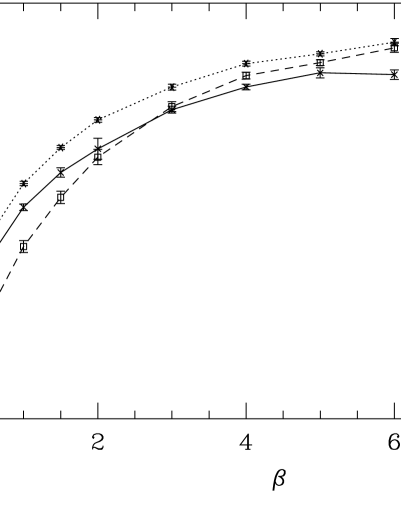
Figure 3: Average link $\langle U\rangle$ as a function of the inverse gauge coupling $\beta$ for U(1) gauge fields in two dimensions, after standard Landau gauge fixing (solid line), Laplacian gauge fixing (dashed line) and Laplacian followed by Landau gauge fixing (dotted line). The lattice size is $20^{2}$.

An obvious quantity to compare is the average link of the gauge fixed gauge field. In fig. 3 the average link $\mbox{$\langle U\rangle$}=\sum_{\mu x}\mbox{Re}\mbox{$\langle U_{\mu x}\rangle$}/V$ is shown for two dimensional U(1) gauge fields, as a function of the inverse gauge coupling $\beta$. If $\langle U\rangle$ is close to one, the configuration should be smooth. The dashed line is the result after Laplacian gauge fixing, the full line is the result after standard Landau fixing. Here we use a checker board relaxation algorithm to maximize the function (5). One sees, that the Laplacian gauge fixing leads to gauge fixed configurations with a larger average link for $\beta\mbox{}_{\textstyle\sim}^{\textstyle>}3$, which roughly corresponds to the scaling region of this model. Only for small $\beta$ the usual Landau fixing produces a larger average link, but even there the difference is not dramatic. The third curve (dots) is obtained by applying Landau gauge fixing after putting the gauge field in the Laplacian gauge. Here we consistently find that the subsequent Landau cooling increases the average link to a somewhat larger value. The standard Landau gauge fixing algorithm is typically unable to find the absolute maximum of (5), and the lattice Landau gauge suffers form Gribov ambiguities, for recent work on lattice Gribov copies, see e.g. ref. [5]. After preconditioning with Laplacian gauge fixing a larger maximum is found, but we have not investigated if this preconditioning actually leads to the absolute maximum.

Similarly we have computed the average link for SU(2) gauge fields in four dimensions. Here we also find little difference between the Laplacian and Landau gauge for $\beta\mbox{}_{\textstyle\sim}^{\textstyle>}2.2$, see fig. 5. To compute the average link shown in fig. 5, we used 8 independent equilibrium configurations and to see the presence of Gribov copies we applied 20 different random gauge transformations to each of them. Typically the average link depends on the initial random gauge transformation of the gauge field, but the differences in the final values of the average link are usually small, less than $\approx 0.005$ for $\beta\mbox{}_{\textstyle\sim}^{\textstyle>}2$, which would be invisible on the scale of fig. 4. For increasing $\beta$ on a fixed lattice size, the number of Gribov copies encountered, decreases and also the difference in values of the average link in the various copies appears to decrease. For smaller values of $\beta$ the ambiguities increase and also the difference between Landau and Laplacian gauge fixed configurations becomes larger.

Figure 4: Average link $\langle U\rangle$ as a function of the inverse gauge coupling $\beta$ for SU(2) gauge fiels in four dimensions, after standard Landau gauge fixing (solid line) and Laplacian gauge fixing (dashed line). The lattice size is $8^{4}$.

The average link singles out the zero momentum mode of the trace of the link field. As in perturbation theory one would like to see that also the other small momentum modes of the gauge fixed field are boosted compared to the high momentum modes. This can be illustrated by computing the Fourier spectrum of the gauge fixed gauge field. In fig. 5 we plot the average value of the coefficients $c_{p}$ of the momentum modes of the SU(2) gauge fixed gauge field,

$$c_{p}^{k}=\mbox{$\langle\left|\sum_{\mu x}u^{k}_{\mu x}e^{-ipx}/4V\right|^{2}\rangle$}^{1/2},$$ (9)

where the $u^{k}$ are the real components of the SU(2) gauge field, $U=i\sum_{k}^{3}\sigma_{k}u^{k}+u^{4}$.

Figure 5: Mean square average of the momentum modes of equilibrium SU(2) gauge fields at $\beta=2.4$ on a $16^{4}$ lattice. The average $u^{4}$ component $c_{p}^{4}$ is shown without gauge fixing (open circles), after Laplacian gauge fixing (boxes) and after Landau gauge fixing (crosses). Similarly the $c_{p}^{1}$ component is shown without gauge fixing (stars), after Laplacian gauge fixing (triangles) and after Landau gauge fixing (three prongs). The results for $c_{p}^{2}$ and $c_{p}^{3}$ are almost indistinguishable from that for $c_{p}^{1}$. To avoid cluttering, we have suppressed some of the momenta for $\hat{p}^{2}>2$.

The modes in fig. 5 are labeled by the value of the lattice momentum $\hat{p}=(\sum_{\mu}(2-2\cos p_{\mu}))^{1/2}$; the lattice size is $16^{4}$ and we used 10 equilibrium configurations at $\beta=2.4$ for the average. The zero momentum mode $c_{0}^{4}$ is responsible for the large value of the expectation value of the average link, which is shown already in fig. 5. One sees that the $u^{k}$ components with $k\not=4$, which represent the three components of the SU(2) gauge potential, are boosted for small momenta $\hat{p}^{2}<2$. The large momentum modes, $\hat{p}^{2}\mbox{}_{\textstyle\sim}^{\textstyle>}2$ of these components as well as all nonzero modes of $u^{4}$ are suppressed, as expected. This is particularly clear in comparison with the result for non-gauge fixed fields. Here it is seen that all momentum components are equally important and the $k\not=4$ modes are indistinguishable from the $k=4$ mode (open circles and stars in fig. 5). Fig. 5 contains both the result for the Landau gauge (open boxes and triangles) and for the Laplacian gauge (crosses and three prongs). It shows that the relative importance of the momentum modes of the gauge fixed field is almost identical in both gauges, over the full range of lattice momenta. For smaller values of $\beta$ this close agreement becomes less.

4 Discussion

In this paper we have performed various tests of the Laplacian gauge fixing prescription. Two important properties claimed in ref. [6] of this gauge are that it is unambiguously computable for almost all gauge fields and that it leads to similarly smooth gauge fixed fields as the Landau gauge.

The Gribov horizons of the Laplacian gauge have measure zero in the gauge field configuration space in the ideal case that the hypersurface where the lowest eigenvalues of the Laplacian cross, or where the eigenvalue on some site vanishes, can be exactly computed. In practice the numerical accuracy $\epsilon$ with which the eigenfunction can be computed, gives the horizons a volume $\propto\epsilon$ and we define the path integral by excluding these Gribov horizon regions. We find that the numerical accuracy of our algorithm is high, leading to a very small $\epsilon$ of order $10^{-10}$.

We have attempted to find how frequently Gribov horizons are encountered in an actual simulation. Using a HMC simulation of U(1) and a Metropolis simulation of SU(2) gauge theory we produced (highly correlated) Markov chains of gauge fields configurations. We never found that the configurations on these chains came within this $\epsilon$ region around the horizons. Only very rarely the two smallest eigenvalues approached each other sufficiently closely that it is likely that the Markov chain actually crossed a Gribov horizon. This suggests that the probability for gauge fields, and hence their ground state wave function, in the regions around the Gribov horizons is small in the cases we have investigated. It is stressed, however, that even if the chain crosses the Gribov horizon, this presents no problem for the gauge fixing algorithm, unless a configurations would accidentally land inside the $\epsilon$ region around the Gribov horizon.

To test the smoothness of the Laplacian gauge fixed configurations, we first showed that for vanishing gauge coupling, $g\rightarrow 0$, the Laplacian gauge reduces to the Landau gauge. We have studied Laplacian gauge fixing numerically for U(1) and SU(2) gauge fields. We find very similar results for the average link and for the relative importance of the various non-zero momentum modes of the Landau and Laplacian gauge fixed configurations. Further more, we find that the Laplacian gauge fixing procedure is rather efficient. When comparing with standard Landau gauge fixing (where we maximize $H$ until its relative change is less than $10^{-12}$) we find that Laplacian gauge fixing typically takes 1-2 times less computer time. These favorable results of Laplacian gauge fixing suggest that, at least on presently used lattice sizes, it is a viable alternative for Landau gauge fixing that could be used to avoid the Gribov ambiguities that afflict the Landau gauge. It would therefore be interesting to repeat e.g. a calculation of glue ball masses with gauge variant glueball operators using the Laplacian gauge and compare the results with those obtained with the Landau gauge.

A disadvantage of Laplacian gauge fixing is that it cannot easily be implemented in perturbation theory. However, this difficulty can perhaps be circumvented by using a Monte Carlo simulation to compute the various two and three point Green functions that are needed to determine e.g. current renormalizations. It may be possible to compute the $\beta$ dependence of these Green functions sufficiently accurately for a range of large values of $\beta$ deep in the perturbative regime, and fit the results to a power series in $1/\beta$. In such a numerical simulation Laplacian gauge fixing could easily be implemented.

Acknowledgement

I would like to thank W. Bock, M. Golterman, J. Hetrick, J. Kuti, S. Sharpe, J. Smit and P. van Baal for discussions. This work is supported by the DOE under grant DE-FG03-91ER40546 and by the TNLRC under grant RGFY93-206.

References

-
[1]
J.E. Mandula and M. Ogilvie, Phys. Lett. B185 (1987) 127;
P. Coddington, A. Hey, J.E. Mandula and M. Ogilvie, Phys. Lett. B197 (1987) 191;
A. Nakamura and R. Sinclair, Phys. Lett. B243 (1990) 396;
C. Bernard, C. Parrinello and A. Soni, Nucl. Phys. B (Proc. Suppl.) 30 (1993) 535. -
[2]
G. Kilcup, Nucl. Phys. B (Proc. Suppl.) 9 (1989) 201;
C. Bernard, A. Soni and K. Yee, Nucl. Phys. B (Proc. Suppl.) 20 (1991) 410;
M.L. Paciello, C. Parrinello, S. Petrarca, B. Taglienti and A. Vladikas, Phys. Lett. B289 (1992) 405. -
[3]
A. Borelli, L. Maiani, G.C. Rossi, R. Sisto and
M. Testa, Phys. Lett. B221 (1989) 360; Nucl. Phys.
B333 (1990) 355;
L. Maiani, Nucl. Phys. B (Proc. Suppl.) 29B,C (1992) 33. - [4] V.N. Gribov, Nucl. Phys. B139 (1978) 1.
-
[5]
A. Nakamura and M. Plewnia, Phys. Lett. 255B (1991) 274.
Ph. de Forcrand, J.E. Hetrick, A. Nakamura and M. Plewnia, Nucl. Phys. B(Proc. Suppl.) 20 (1991) 194.
E. Marinari, C. Parrinello, R. Ricci, Nucl. Phys. B362 (1991) 487;
C. Parrinello, S. Petrarca, A. Vladikas, Phys. Lett. B268 (1991) 236;
M.L. Paciello, C. Parrinello, S. Petrarca, B. Taglienti, A. Vladikas, Phys. Lett. B276 (1992) 163; B281 (1992) 417 (Erratum);
V.G.Bornyakov, V.K. Mitryushkin, M. Müller-Preußker, F. Pahl, Phys. Lett. B317 (1993) 596;
M.I. Polikarpov, K. Yee and M.A. Zubkov, Phys. Rev. D48 (1993) 3377;
P Marenzoni and P. Rossi, Phys. Lett. B311 (1993) 219;
I. Montvay, Phys. Lett. B323 (1994) 378. - [6] J.C. Vink and U.-J. Wiese, Phys. Lett. B289 (1992) 122.
- [7] J.C. Vink, Phys. Lett. B321 (1994) 239.