hep-lat/9406018

UCSD/PTH 94-08

June 1994

Failure of the Regge approach in two

dimensional quantum gravity

Wolfgang Bock        and       Jeroen C. Vink

bock@sdphjk.ucsd.edu               vink@yukawa.ucsd.edu

University of California, San Diego

Department of Physics-0319

9500 Gilman Drive, La Jolla, CA 92093-0319

USA

Abstract

Regge’s method for regularizing euclidean quantum gravity is applied to two dimensional gravity. We use two different strategies to simulate the Regge path integral at a fixed value of the total area: A standard Metropolis simulation combined with a histogramming method and a direct simulation using a Hybrid Monte Carlo algorithm. Using topologies with genus zero and two and a scale invariant integration measure, we show that the Regge method does not reproduce the value of the string susceptibility of the continuum model. We show that the string susceptibility depends strongly on the choice of the measure in the path integral. We argue that the failure of the Regge approach is due to spurious contributions of reparametrization degrees of freedom to the path integral.

1 Introduction

It is still an unsolved problem how a quantum theory of gravitation can be formulated using an euclidean path integral. Well-known problems are the unboundedness of the euclidean action, the perturbative non-renormalizability of the Einstein-Hilbert action and finding a consistent regularization, for instance by discretizing space-time, such that the path integral can be studied non-perturbatively with numerical methods. Here we shall focus on the problem of finding a regularization of the euclidean path integral.

Most studies so far have either used dynamical triangulation [1, 2] or Regge calculus [3]. For recent review articles we refer the reader to refs. [4, 5]. For an approach along a different line, see refs. [6, 7]. In both cases the path integral is replaced by a summation over simplicial manifolds. These simplicial manifolds are built up from $d$ dimensional simplices, triangles in $d=2$ dimensions, which are glued together along their $d-1$ dimensional subsimplices, the edges in two dimensions. In the dynamical triangulation approach one keeps the edge lengths fixed and replaces the integration in the path integral by a summation over simplicial structures with all possible connectivities and numbers of simplices. In the Regge method the edge lengths are the dynamical degrees of freedom, while the connectivities are usually kept fixed. Here the path integral is replaced by an integration over the edge lengths. Both formulations have appealing features, but are also subject to criticism.

In both approaches the metric tensor field, which is the integration variable in the continuum path integral, is replaced by a simplicial structure. With dynamical triangulation, the Einstein-Hilbert action is automatically bounded from below; in the Regge approach one usually adds a curvature square term to make the action bounded [8]. It is far from clear, however, how the continuum integration measure, which includes gauge fixing and Faddeev-Popov terms, has to be translated to a summation over these simplicial structures.

With dynamical triangulation a natural choice is to simply sum over all triangulated surfaces, only weighted by the action. Since it is impossible to use dynamical triangulation to study small fluctuations around a flat space in perturbation theory, the only way to test this conjecture is through numerical simulations. This should reveal the existence of a second order phase transition at which renormalized quantities, such as the volume and curvature fluctuations, become independent of the details of the underlying discrete structure. Studies of the phase structure have given some evidence for the existence of such a critical point in four dimensions [9, 10], but the situation is far from clear [11, 12]. It has furthermore been questioned if the Monte Carlo methods which are presently in use are ergodic [13]. The strongest support for the dynamical triangulation approach comes from its success in two dimensional gravity. Here it has been shown in detail, that the results of the continuum theory are reproduced [4, 5, 14].

In the Regge approach it is less easy to choose a natural measure for the integration over the link lengths. In contrast to the dynamical triangulation approach, it is possible to study the Regge path integral in perturbation theory. Here it has been shown that the path integral with a simple (scale invariant) measure, corresponds to the continuum path integral without gauge fixing or Faddeev-Popov terms [15]. This suggests that also outside perturbation theory, the integration includes degrees of freedom which correspond to coordinate transformations; we shall discuss this in more detail below. To remove these spurious degrees of freedom, one would expect that the measure should include gauge fixing and Faddeev-Popov terms. One has often commented on this issue, but in actual simulations only the scale invariant measure or simple variations thereof have been used.

Even though the justification of the measure used in dynamical triangulation appears to be equally obscure as in the Regge approach, this latter approach has been lacking the compelling success of the dynamical triangulation method in two dimensional gravity. This has motivated some time ago an investigation of the Regge approach in two dimensional gravity [16]. This numerical study claimed that also the Regge method reproduces correctly the scaling of the partition function, in particular the so-called string susceptibility of two dimensional continuum gravity with central charge zero was found. The string susceptibility was not found to coincide with the continuum prediction for non-zero central charge. In the present work we describe the results of a similar study of the central charge zero model, which we believe improves several of the shortcomings of ref. [16]. We shall use the same Regge action, which includes an $R^{2}$ term, and the same scale invariant integration measure as in ref. [16]. Unfortunately, we find wrong values for the string susceptibility, when the simplicial structure has the topology of a sphere or a “bi-torus” (a manifold with two handles). We will show explicitly that the scaling of the Regge partition function depends very sensitively on the details of the integration measure.

The paper is organized as follows. In sect. 2 we review the continuum scaling relations for the path integral over surfaces with a fixed area. We discuss in some detail how the Regge skeletons can be viewed as discretizations of the metric field of continuum manifolds. Sect. 3 deals with the derivation of scaling relations for the Regge path integral over skeletons with a fixed area. We shall show that these scaling relations reveal a sensitive dependence of the string susceptibility on the integration measure. In sect. 4 we discuss the technical aspects of our simulation methods. As a novelty, a Hybrid Monte Carlo algorithm is introduced which can be used to simulate the fixed area Regge path integral. Our numerical results are presented in sect. 5 and a brief summary and some final remarks are contained in sect. 6.

2 Regge approach to two dimensional gravity

2.1 Continuum scaling relations

Let us consider the euclidean path integral for two dimensional pure gravity (the central charge zero model),

$$Z(A) = \int\frac{{\cal D}g}{{\rm Vol(Diff)}}\;e^{-S(g)}\;\delta(\int d^{2}x\sqrt{g}-A)\;,$$ (2.1)

$$S(g) = \int d^{2}x\;\sqrt{g}\;(\lambda+\kappa R+\beta R^{2})\;.$$ (2.2)

In two dimensions the curvature term $\int d^{2}x\sqrt{g}R=4\pi\chi$ is a topological invariant (Gauss-Bonnet theorem) depending only on the Euler characteristic $\chi=2(1-h)$, where $h$ denotes the number of handles or genus of the surface. The genus is zero for the sphere, one for the torus and two for the bi-torus. We have included a $R^{2}$ term in the action with a coupling constant $\beta$ which has a dimension of 1/mass². The coupling constant $\kappa$ is dimensionless and the cosmological constant $\lambda$ has a dimension of mass². The delta function in (2.1) imposes the constraint that the area of the surface is equal to $A$. Formally the measure is normalized by the infinite volume of the diffeomorphism group, which should cancel the infinite factor that arises from the integration over the gauge (reparametrization) degrees of freedom in the path integral. The continuum measure ${\cal D}g$ is ill-defined because it involves an infinite product over all space-time points.

On a formal level, i.e. ignoring the measure, one would expect that

$$Z(A)\propto A^{-1}\exp[-\lambda A]\;,$$ (2.3)

if we set $\beta$ in the action (2.2) equal to zero. However, after regularization and fixing the gauge using the usual Faddeev-Popov procedure, one finds that the measure breaks the conformal (scale) symmetry and the $A$ dependence of the partition function is given by

$$Z(A)\propto A^{\gamma_{{\rm str}-3}}\exp[-\lambda_{R}A]\;,$$ (2.4)

where $\lambda_{R}$ is the renormalized cosmological constant. The string susceptibility $\gamma_{{\rm str}}$ depends on the genus $h$ of the surface,

$$\gamma_{{\rm str}}=2-\frac{5}{2}\;(1-h)\;.$$ (2.5)

The relations (2.4) and (2.5) were first derived for the special case $h=0$ using the light cone gauge [17] and were later confirmed [18] and generalized to topologies of arbitrary genus $h$ [19] using the conformal gauge. Quantum fluctuations are seen to lead to a deviation from the naive scaling dimension of the partition function for $h\neq 1$ and renormalize the cosmological constant.

For small, but non-zero $\beta$ one expects that the result (2.4) remains valid in the regime where $A\gg 1/\beta$, because the $R^{2}$ term should only modify the short distance behavior of the theory. The $R^{2}$ model for $A/\beta\rightarrow 0$ has been studied in ref. [20]. Using the dynamical triangulation method it has been demonstrated numerically that the addition of a small $R^{2}$ term did not affect the value of the string susceptibility [2, 21].

In order to study this two dimensional gravity model using the Regge regularization, one first has to express the action (2.2) in terms of the edge lengths and then integrate over all length variables with an appropriate choice for the measure. In order to expose more clearly the role of reparametrization invariance we shall recall briefly that the Regge action can be viewed as a discretization of the continuum Einstein-Hilbert action. This establishes a link between the edge lengths of a Regge skeleton and the metric field in the continuum and furthermore sheds light on the problem of choosing the integration measure in the Regge approach.

2.2 Regge discretization

Usually the Regge skeletons are considered as special, piecewise flat, continuum manifolds. Here we want to take a somewhat different point of view, in which a Regge skeleton is a discretized version of an underlying continuum manifold which is defined by a metric tensor field $g_{\mu\nu}(x)$. For simplicity we shall assume that the continuum manifold $T$ has the topology of a torus. Then we can choose global coordinates $\{x=(x_{1},x_{2})\}$ on this surface with metric $g_{\mu\nu}(x)$. The coordinates are a (globally defined) map from a flat unit torus $T_{0}=\{x|x_{1}\in[0,1),x_{2}\in[0,1)\}$, into the curved surface of $T$. We can construct a grid on the curved torus $T$ by first defining the grid $\Lambda=\{x|x_{\mu}=n_{\mu}a_{0};n_{\mu}=1,\cdots,N;a_{0}=1/N\}$ on $T_{0}$, as shown in fig. 1 and then mapping it onto the curved surface. In this way we can obtain triangulations of $T$ where the triangles are spanned by the triplets of coordinates $\{(n_{1}a,n_{2}a)$, $((n_{1}+1)a,n_{2}a),((n_{1}+1)a,(n_{2}+1)a)\}$ and $\{(n_{1}a,n_{2}a),(n_{1}a,(n_{2}+1)a),((n_{1}+1)a,(n_{2}+1)a)\}$, cf. fig. 1.

Figure 1: Triangulation of the torus with $N=4$. The boundaries with the same labels have to be identified. The lattice spacing is denoted by $a_{0}$. Each vertex in the skeleton has coordination number six.

The edge lengths to be used in the Regge skeleton, can be defined in various ways: one can take the proper length of images of the corresponding edges on the unit torus $T_{0}$, one can use the geodesic distance or one can use the distances in some flat embedding space.

Using such a construction, one can give the relation between the continuum metric $g_{\mu\nu}$ and the link lengths of the Regge skeleton,

$$l_{1i} = \sqrt{g_{11}}\;a_{0}+O(a_{0}^{2}),$$

$$l_{2i} = \sqrt{g_{22}}\;a_{0}+O(a_{0}^{2}),$$

$$l_{3i} = \sqrt{g_{11}+2g_{12}+g_{22}}\;a_{0}+O(a_{0}^{2}),$$ (2.6)

where $a_{0}=1/N$ is the lattice distance on the unit torus $T_{0}$. The metric tensor $g_{\mu\nu}$ in (2.6) is evaluated at the site $x_{i}=(n_{1}a_{0},n_{2}a_{0})\in\Lambda$ and the three links $l_{1i}$, $l_{2i}$ and $l_{3i}$ are the edges on $T$ that are associated with the coordinate pairs $\{(n_{1}a_{0},n_{2}a_{0})$, $((n_{1}+1)a_{0},n_{2}a_{0})\}$, $\{(n_{1}a_{0},n_{2}a_{0}),(n_{1}a_{0},(n_{2}+1)a_{0})\}$ and $\{(n_{1}a_{0},n_{2}a_{0})$, $((n_{1}+1)a_{0},(n_{2}+1)a_{0})\}$, respectively (see fig. 1).

Let us now for a moment take the more common point of view and consider the skeleton we have constructed above as a piecewise flat manifold, and not as a discretization of a continuum manifold. The curvature is then concentrated at the vertices and is given by $\sum_{i}\delta_{i}\delta(x-x_{i})$ [3], where $\delta_{i}$ is the deficit angle at the vertex $x_{i}$. The deficit angle $\delta_{i}$ is given by $\delta_{i}=2\pi-\sum_{t}\phi_{t}$, where $\phi_{t}$, $t=1,\ldots,6$ are the six dihedral angles that meet at site $x_{i}$. From the point of view that a skeleton represents an approximation of an underlying smooth continuum manifold, such a singular curvature distribution is unnatural. Rather we should approximate the curvature in a region $A_{i}$ around the vertex $x_{i}$ by a constant $R_{i}$, such that $R_{i}A_{i}=\int_{A_{i}}d^{2}x\sqrt{g(x)}R(x)$. This implies that

$$R_{i}=2\delta_{i}/A_{i}\;.$$ (2.7)

There is no unique prescription to assign an area $A_{i}$ to a vertex $x_{i}\in T_{0}$. The easiest way is to follow ref. [8] and use a baricentric subdivision where one divides each triangle on $T$ along the side bisections into three equal pieces. The area $A_{i}$ associated with the vertex $x_{i}$ is then given by

$$A_{i}=\mbox{{\small$\frac{1}{3}$}}\sum_{t=1}^{6}A_{it}\;,$$ (2.8)

where $A_{it}$, $t=1,\ldots,6$ are the six triangle areas connected to the vertex $i$. For a given triangle with edge lengths $l_{\alpha}$, $l_{\beta}$ and $l_{\gamma}$, the triangle area $A_{\alpha\beta\gamma}$ and the dihedral angle $\phi_{\gamma}$ which is opposite to the edge $l_{\gamma}$ are given by

$$A_{\alpha\beta\gamma}\;\; = \;\;\mbox{{\small$\frac{1}{4}$}}\sqrt{-l_{\alpha}^{4}-l_{\beta}^{4}-l_{\gamma}^{4}+2(l_{\alpha}^{2}l_{\beta}^{2}+l_{\beta}^{2}l_{\gamma}^{2}+l_{\alpha}^{2}l_{\gamma}^{2})}$$ (2.9)

$$\phi_{\gamma}\;\; = \;\;\arccos\left(\frac{l_{\alpha}^{2}+l_{\beta}^{2}-l_{\gamma}^{2}}{2l_{\alpha}l_{\beta}}\right)\;.$$ (2.10)

With the replacement $R(x)\rightarrow 2\delta_{i}/A_{i}$ for $x\in A_{i}$ it is also straightforward to discretize the $R^{2}$ term [8] which poses a problem on a piecewise flat manifold because one cannot square the delta functions. This leads to the Regge form of the action (2.2),

$$S(l)=\sum_{i}\left\{\lambda A_{i}+2\kappa\delta_{i}+4\beta\delta_{i}^{2}/A_{i}\right\}\;,$$ (2.11)

with $2\sum_{i}\delta_{i}=4\pi\chi$ the discrete version of the Gauss-Bonnet theorem. For a given torus with a sufficiently smooth metric field, this discretized Regge action approaches the continuum action (2.2) in the limit that the regularization is removed. It can be checked, for instance using the Mathematica package, that $A_{i}=\sqrt{g(x_{i})}a_{0}^{2}+O(a_{0}^{3})$ and $R_{i}=R(x_{i})+O(a_{0})$, when expressing the edge lengths in eqs. (2.7) and (2.8) in terms of the metric, using relations (2.6), and expanding to leading order in $a_{0}$.

The above discretization procedure is not invariant under general coordinate transformations on $T$. Let us illustrate this for the cosmological term. Using the relations (2.6) and (2.9) we can express the sum in (2.8) in terms of $g_{\mu\nu}$,

$$A_{i}\!\! = \!\!a_{0}^{2}\;\sqrt{g}+\frac{a_{0}^{3}}{4\sqrt{g}}\left\{-g_{11}\;\partial_{x_{2}}g_{22}-g_{22}\partial_{x_{1}}g_{11}\right.$$ (2.12)

$$\!\!\left.+g_{12}(\partial_{x_{1}}g_{22}+\partial_{x_{2}}g_{11})+2g_{12}(\partial_{x_{1}}+\partial_{x_{2}})g_{12}\right\}+O(a_{0}^{4})\;,$$

with the metric and its derivatives evaluated at the point $x_{i}=(n_{1},n_{2})$. The relation (2.12) shows that the general coordinate or diffeomorphism invariance is broken by the $O(a_{0})$ terms in the action. This implies that a given set of continuum manifolds which are related by general coordinate transformations on $T$ will lead to Regge skeletons whose actions differ by $O(a_{0})$ effects.

There are two sources of discretization effects when translating a continuum manifold into a Regge skeleton in the above way: Firstly, of course, discretization effects depend on the value of $N$. Secondly, the discretization effects depend on the choice of coordinates on $T$. By choosing an optimal coordinate system, one can minimize the discretization effects at a given $N$. For instance, one could choose a gauge fixing condition that minimizes the square of the terms in the action which are $\propto a_{0}^{3}$ (cf. eq. (2.12)).

According to the picture sketched above, the edge lengths in a Regge skeleton represent both physical degrees of freedom, corresponding to curvature fluctuations, and gauge degrees of freedom, corresponding to coordinate reparametrizations. Since in general there does not exist a transformation which is an invariance of the Regge action (2.11), the identification of a “gauge transformation” on the edge lengths is necessarily ambiguous. For instance, such gauge transformations on $l$ may be defined as

$$l_{1}\!\! \rightarrow \!\!\left[l_{1}^{2}+2\partial^{\prime}_{1}\xi_{1}\right]^{1/2},$$

$$l_{2}\!\! \rightarrow \!\!\left[l_{2}^{2}+2\partial^{\prime}_{2}\xi_{2}\right]^{1/2},$$

$$l_{3}\!\! \rightarrow \!\!\left[l_{3}^{2}+2\partial^{\prime}_{1}\xi_{1}+2\partial^{\prime}_{2}\xi_{2}+2(\partial^{\prime}_{1}\xi_{2}+\partial^{\prime}_{2}\xi_{1})\right]^{1/2}\;,$$ (2.13)

where $\partial^{\prime}_{\mu}\xi_{\nu}=(\xi_{\nu,i+\hat{\mu}}-\xi_{\nu,i})/a_{0}$. This transformation is constructed such that after inserting relations (2.6) into (2.13), one recovers from the leading order terms in $\xi$ the infinitesimal continuum gauge transformations, $g_{\mu\nu}\rightarrow g_{\mu\nu}+\partial_{\mu}\xi_{\nu}+\partial_{\nu}\xi_{\mu}$. The transformations (2.13) are associative, i.e. $l^{\xi+{\xi}^{\prime}}=(l^{\xi})^{\xi^{\prime}}$. This is an important property since it allows us to devide the configuration space of Regge skeletons into equivalence classes $l^{\xi}$ (gauge orbits), that consist of skeletons which are related by a gauge transform of the form (2.13).

2.3 Integration measure

Next we turn to the problem of defining the measure for the integration over Regge skeletons in the path integral. In the continuum path integral, the measure (before gauge fixing) is of the form

$${\cal D}g=\prod_{x}g(x)^{3\alpha}\prod_{\mu\geq\nu}dg_{\mu\nu}(x)\;.$$ (2.14)

For $\alpha=-1/2$ this measure is scale invariant, for $\alpha=-1/4$ it is gauge invariant as follows from Fujikawa’s method [22]. One could now use the relation (2.6) to regularize this measure by expressing it in terms of the edge lengths $l$,

$$g(x)^{3\alpha}\prod_{\mu\geq\nu}dg_{\mu\nu}(x)\rightarrow d\mu(l)=\mbox{{\normalsize$\frac{1}{2}$}}[2A_{123}(l)]^{3\alpha}\prod_{\beta=1}^{3}dl_{\beta}^{2}\;,$$ (2.15)

where we have suppressed the site index $i$. The triangle area $A_{123}$ is defined in (2.9). Such a measure includes the gauge degrees of freedom. In the continuum the gauge degrees of freedom are removed by gauge fixing and the full measure would acquire an additional gauge fixing and Faddeev-Popov term. For the integration over Regge skeletons one is not forced to fix the gauge because the gauge invariance is broken by the the discretization procedure and no infinite volume of the diffeomorphism group can arise.

At this point one can follow two strategies: One can ignore the gauge degrees of freedom (the $\xi$’s of eqs. (2.13)) and hope that these modes decouple automatically from the physical degrees of freedom when approaching the continuum limit. Small $\xi$ fluctuation are indeed almost decoupled, when the Regge skeleton is sufficiently smooth as has been demonstrated in ref. [15], but for a generic skeleton they are strongly coupled and it is difficult to believe that they can ever decouple from the physical degrees of freedom in a non-perturbative evaluation of the path integral. For a discussion of this scenario of dynamical gauge symmetry restoration in the context of a non-perturbative formulation of chiral gauge theories on the lattice, see ref. [23].

The second strategy one could follow, is to mimic the continuum approach. This implies that the gauge degrees of freedom should be removed from the path integral by employing a suitable gauge fixing and Faddeev-Popov procedure. To implement this in the Regge path integral, one could translate the continuum gauge fixing term and corresponding Faddeev-Popov ghost term into a Regge form, e.g. using the correspondence (2.6). In the continuum the BRST symmetry prevents that gauge non-invariant terms emerge in the low energy theory; on the lattice this symmetry is not present and one expects that gauge non-invariant counter terms have to be added in order to recover a BRST invariant low energy theory. Such an approach has been advocated some time ago for the lattice regularization of chiral gauge theories [24], which also have the difficulty that the local gauge symmetry is broken by the regularization. The technical problem with this approach is that the ghost term in the action is very hard to include in a numerical Monte Carlo evaluation of the path integral and a non-perturbative computation of the counterterm coefficients may be very cumbersome.

This second option appears to have the best chance of leading to a well-defined path integral, since it should work at least in perturbation theory. However, faced with the technical difficulties of this strategy, previous studies of the Regge path integral have resorted to the first (non-gauge fixing) approach. The integration measure was chosen to be of a very simple form

$$d\mu_{\zeta}(l)=\prod_{\alpha,i}\frac{dl_{\alpha i}^{2}}{l_{\alpha i}^{2}}\;l_{\alpha i}^{\zeta}\;,$$ (2.16)

which is scale invariant for $\zeta=0$. For a recent investigation of the $\zeta$ dependence of expectation values of local observables see ref. [25].

3 Regge scaling relations

Consider now the path integral for Regge skeletons with a fixed area $A$,

$$Z(A,N_{1})=\int d\mu_{\zeta}(l)\;F(l)\;\exp\left[-\sum_{i}(\lambda\;A_{i}+\beta\;R^{2}_{i})\right]\delta(\sum_{i}A_{i}-A)\;,$$ (3.1)

where we use the abbreviation $R_{i}^{2}=4\delta^{2}_{i}/A_{i}$. The total curvature of a skeleton is $4\pi\chi$ and we leave this term out from the action since we shall study only skeletons with a fixed topology. The measure $d\mu_{\zeta}(l)$ is of the simple form (2.16) and is scale invariant for $\zeta=0$. The factor $F(l)$ is equal to zero if the skeleton contains one or more triangles for which the triangle inequalities are violated, and is one otherwise. We have in (3.1) included the argument $N_{1}$, which is the number of edges (1-simplices) in the skeleton, to indicate that we evaluate the path integral for a fixed number of edges with fixed connectivities.

To eliminate the delta function, we first perform a transformation of variables,

$$l_{\alpha i}\rightarrow\sqrt{s}\;l_{\alpha i}\;.$$ (3.2)

Since $F(l)$ which imposes the triangle inequalities is unaffected by this change of integration variables, eq. (3.1) can be written in the form

$$Z(A,N_{1})=\int d\mu_{\zeta}(\sqrt{s}l)\;F(l)\;\exp\left[-\sum_{i}(\lambda\;s\;A_{i}+\frac{\beta}{s}\;R^{2}_{i})\right]\delta(s\;\sum_{i}A_{i}-A)\;.$$ (3.3)

Since the partition function $Z(A,N_{1})$ does not depend on $s$ we may integrate both sides in (3.3) over $s$ with a normalized weight function $P(s)$, i.e. $\int_{0}^{\infty}dsP(s)=1$,

$$\!\!\!\!\!\!\!\!\!\!\!\!Z(A,N_{1})=\int d\mu_{\zeta}(l)F(l)\int dss^{N_{1}\zeta/2}P(s)\exp\left[-\sum_{i}(\lambda sA_{i}+\frac{\beta}{s}R^{2}_{i})\right]\delta(s\sum_{i}A_{i}-A)$$

$$\!\!\!\!\!\!\!\!\!\!\!\!=\exp[-\lambda A]\int d\mu_{\zeta}(l)F(l)\frac{1}{\sum_{i}A_{i}}\left(\frac{A}{\sum_{i}A_{i}}\right)^{N_{1}\zeta/2}P\left(\frac{A}{\sum_{i}A_{i}}\right)\exp\left[-\frac{\beta}{A}\sum_{j}A_{j}\;\sum_{i}R^{2}_{i}\right]\;$$

$$\!\!\!\!\!\!\!\!\!\!\!\!\equiv\int d\mu_{\zeta}(l)\;F(l)\;\exp[-S^{{\rm scale}}(l)]\;,$$ (3.4)

where the last equality defines the rescaled action $S^{{\rm scale}}(l)$.

Now it appears as if $Z(A,N_{1})$ depends on the arbitrary function $P$, but this is of course not the case. This follows from an infinite set of Ward identities which can be derived by using again the scale transformation (3.2), and observing that $d^{n}Z(A,N_{1})/ds^{n}=0$, $n=1,2,3,\ldots$. For $n=1$ this gives the identity

$$\left\langle\frac{A}{\sum_{i}A_{i}}P^{\prime}\left(\frac{A}{\sum_{i}A_{i}}\right)\left/\right.P\left(\frac{A}{\sum_{i}A_{i}}\right)\right\rangle=-1\;,$$ (3.5)

where the expectation value is with respect to the rescaled action,

$$\mbox{$\langle\bullet\rangle$}=Z(A,N_{1})^{-1}\int d\mu_{\zeta}(l)\;F(l)\;\bullet\;\exp[-S^{{\rm scale}}(l)]\;.$$ (3.6)

We want to investigate if the Regge partition function $Z(A,N_{1})$ reproduces the scaling behavior (2.4) in the continuum limit, i.e. for $N_{1}\rightarrow\infty$. Therefore it is useful to consider the derivative

$$\frac{d\log Z(A,N_{1})}{dA}=-\lambda+\frac{1}{A}\left(\frac{\beta}{A}\mbox{$\langle\sum_{j}A_{j}\sum_{i}R^{2}_{i}\rangle$}+\frac{N_{1}\zeta}{2}-1\right)\;,$$ (3.7)

with $\lambda\beta$ and $N_{1}$ kept fixed. Here we have used the identity (3.5) to eliminate a $P^{\prime}/P$ term.

Next we note that the expectation value $\langle\sum_{j}A_{j}\;\sum_{i}R^{2}_{i}\rangle$ is a function of the ratio $\beta/A$ and of $N_{1}$. This follows from inspecting the path integral (3.4). If for $N_{1}\rightarrow\infty$ this expectation value behaves such that

$$\frac{\beta}{A}\;\mbox{$\langle\sum_{j}A_{j}\;\sum_{i}R^{2}_{i}\rangle$}+\frac{N_{1}\zeta}{2}=-\frac{A}{\beta}\;\delta\lambda+\delta\gamma+O(\frac{\beta}{A})\;,$$ (3.8)

then the Regge partition function would scale as

$$Z(A,\infty)\propto\exp\left[-\left(\lambda+\frac{\delta\lambda}{\beta}\right)A\right]A^{-1+\delta\gamma}$$ (3.9)

and we may identify $\lambda+\delta\lambda/\beta$ with the renormalized cosmological constant and $\delta\gamma+2$ with the string susceptibility $\gamma_{{\rm str}}$.

Since the term $(\beta/A)\sum_{j}A_{j}\;\sum_{i}R^{2}_{i}$ is the total action in the path integral (3.4), its expectation value in general will grow proportionally to $N_{1}$. Hence the limit $N_{1}\rightarrow\infty$ only exists, if the exponent $\zeta$ in the measure is chosen such that $N_{1}\zeta/2$ cancels the term $\propto N_{1}$ in the expectation value of the action.

Instead of the measure (2.16) we could also have used a different measure where the exponent $\zeta$ is given by $\zeta=\zeta_{0}+\zeta_{1}/N_{1}$. Now the term $N_{1}\zeta_{0}/2$ has to cancel the divergence, but the finite part is shifted by the arbitrary constant $\zeta_{1}$ which gives a contribution to the string susceptibility. Hence $\delta\gamma$ appears to depend very sensitively on the choice of the measure. The only way that $\delta\gamma$ could be independent of $\zeta_{1}$ is if it is compensated by the expectation value of the action: An expansion to lowest order in $\zeta_{1}/N_{1}$ shows that $\gamma_{{\rm str}}$ is shifted by $\zeta_{1}(\mbox{{\normalsize$\frac{1}{2}$}}+c)$ with $c$ the connected part of $\langle(\sum_{\alpha,i}\log l_{\alpha i})(\sum_{j}A_{j}\sum_{i}\beta R_{i}^{2}/A)\rangle$, evaluated for $\zeta_{1}=0$. It is very unlikely that $c$ is exactly equal to $-1/2$, such that $\delta\gamma$ is independent of $\zeta_{1}$.

This sensitive dependence of $\delta\gamma$ on the measure is seen particularly clearly for $\beta=0$: Then eq. (3.7) can be integrated easily, giving

$$Z(A,N_{1})\propto A^{-1+N_{1}\zeta_{0}/2+\zeta_{1}/2}\;\exp[-\lambda A]\;.$$ (3.10)

For the choice $\zeta_{0}=0$ the limit $N_{1}\rightarrow\infty$ can be taken and the partition function is of the same form as in the continuum, but with an arbitrary string susceptibility $\gamma_{{\rm str}}=2+\zeta_{1}/2$.

This discussion shows that the real difficulty is the lack of a criterion to fix such ambiguities. This is different in the continuum where the power $\zeta$ is fixed in Fujikawa’s method [22], by the requirement of gauge invariance. Such a guideline is lacking in the Regge model.

These considerations cast serious doubts on the claim made in ref. [16] that the Regge model with scale invariant measure reproduces the continuum values of the string susceptibility. To settle this, we have also performed a numerical simulation of this model using the scale invariant measure, i.e. for $\zeta=0$, and three different topologies with genus $h=0,1$ and $2$. We shall see that the numerical estimates for $\gamma_{{\rm str}}$ differ substantially from the continuum result for $h\neq 1$.

4 Details of the numerical simulation

4.1 Histogramming

The area dependence of the Regge partition function can be inferred from eq. (3.7) by computing $\langle(\beta/A)\sum_{j}A_{j}\sum_{i}R^{2}_{i}\rangle=-\beta d\log Z(A,N_{1})/d\beta$ in the rescaled model (3.4). This is identical to evaluating the expectation value of $\beta R^{2}$ in the original model with the delta function (3.1). Hence there are two ways to proceed: One can simulate either the original model, including the delta function that constraints the area to be fixed, or alternatively one can simulate the rescaled model (3.4).

The first option poses the problem of including the constraint that the total area must be fixed. Such a global constraint is hard to implement efficiently in a Monte Carlo simulation (see however ref. [26]). Alternatively it is possible to include the constraint a posteriori. To this extend we first approximate the delta function by a narrow block function which is normalized to one,

$$\Delta_{h}(A)=\left\{\begin{array}[]{ll}\frac{1}{2h}\;,&\mbox{if}\;\;A\in[-h,h]\\ 0\;,&\mbox{if}\;\;A\not\in[-h,h]\;.\end{array}\right.$$ (4.1)

Then the expectation value of the observable $O(l)$ is given by,

$$\mbox{$\langle O\rangle$}_{A}\!\! = \!\!Z(A,N_{1})^{-1}\int\;d\mu_{\zeta}(l)\;F(l)\;O(l)\;\Delta_{h}(\sum_{i}A_{i}-A)\;\exp[-S(l)]$$ (4.2)

$$= \!\!\mbox{$\langle O(l)\;\Delta_{h}(\sum_{i}A_{i}-A)\rangle$}/\mbox{$\langle\Delta_{h}(\sum_{i}A_{i}-A)\rangle$}\;,$$

where the action $S(l)$ is given in eq. (2.11) with $\kappa=0$ and $\langle\bullet\rangle$ in the lower line is evaluated in the model without the area constraint. In practise this amounts to generating an equilibrium ensemble of skeletons with the unconstraint action and then computing the average of $\beta R^{2}$ on the subensemble for which the total area is within the interval $[A-h,A+h]$ for a selected value of $A$. We shall refer to this method as “the histogramming technique”.

Most of our numerical results to be presented below, have been obtained with this method. For the simulation of the unconstraint action we use a Metropolis algorithm. The $R^{2}$ term in the Regge action extends over several triangles and in order to make the code vectorizable we had to use a four color subdivision of the lattice. In the model without the area constraint we can derive the Ward identity

$$\!\!\!\!\!\!\!\!\!-\frac{N_{1}\zeta}{2}+\frac{1}{Z}\int d\mu_{\zeta}\;F(l)\;\left(\lambda\;\sum_{i}A_{i}-\beta\;\sum_{i}R^{2}_{i}\right)\exp[-S(l)]=0\;,$$ (4.3)

$$\!\!\!\!\!\!\!\!\!Z=\int d\mu_{\zeta}\;F(l)\;\exp[-S(l)]\;,$$ (4.4)

which follows from the invariance under rescaling of the links. This shows that the unconstraint path integral is divergent for $\zeta=0$ and $\beta=0$ because the expectation value of $\sum_{i}A_{i}>0$ can only vanish if (4.4) diverges. This is perhaps seen even more clearly by writing the unconstraint partition function in the form $Z=\int_{0}^{\infty}dA\;Z(A,N_{1})$ with $Z(A,N_{1})$ given in eq. (3.1). The integration of relation (3.7) for $\beta=0$ yields $Z(A,N_{1})\propto A^{\zeta/2-1}\;\exp[-\lambda A]$, which shows that the unconstraint partition function $Z$ has a non-integrable singularity at $A=0$ if $\zeta\leq 0$.

Also the rescaled action (3.4) could be simulated using a Metropolis algorithm. However, the non-local action $\beta\sum_{j}A_{j}\sum_{i}R^{2}_{i}$ prevents vectorization of the code. This suggests to use a Hybrid Monte Carlo algorithm, which can easily be vectorized and is usually found to be more efficient than a Metropolis algorithm.

4.2 Hybrid Monte Carlo algorithm

To use the Hybrid Monte Carlo algorithm we first introduce new degrees of freedom $p_{\alpha i}$ which are viewed as the canonical momenta of the edge lengths $l_{\alpha i}$ with respect to the measure $dl_{\alpha i}\;dp_{\alpha i}$. The path integral (3.4) may then be written in the form

$$Z\!\! = \!\!\int\prod_{\alpha,i}(dl_{\alpha i}\;dp_{\alpha i})\;F(l)\;\exp[-H(l,p)]\;,$$ (4.5)

$$H(l,p)\!\! = \!\!\mbox{{\normalsize$\frac{1}{2}$}}\sum_{\alpha,i}p_{\alpha i}^{2}+\hat{S}(l)\;,$$ (4.6)

$$\hat{S}(l)\!\! = \!\!\frac{\beta}{A}\;\sum_{j}A_{j}\;\sum_{i}R^{2}_{i}-\ln P\left(\frac{A}{\sum_{i}A_{i}}\right)$$ (4.7)

$$\!\!+(\mbox{{\normalsize$\frac{1}{2}$}}\;N_{1}\;\zeta+1)\;\ln\left(\sum_{i}A_{i}\right)-(\zeta-1)\;\sum_{\alpha,i}\ln l_{\alpha i}\;,$$

where we have introduced the hamiltonian $H(l,p)$ and dropped the constant $\lambda A-\mbox{{\normalsize$\frac{1}{2}$}}N_{1}\zeta\ln A$ from $\hat{S}(l)$. The various factors in (3.4) have been included as logarithms in the action, except for $F(l)$ which is a discontinuous function of the edge length $l$.

We now want to find trajectories for $l(t)$ and $p(t)$ such that the hamiltonian $H(l,p)$ is conserved in the (computer) time $t$. After choosing the canonical relation

$$\frac{dl}{dt}=\frac{\partial H(l,p)}{\partial p}=p\;,$$ (4.8)

we can compute the time derivative of $p$ from the requirement that $dH/dt=0$, which leads to

$$\frac{dp_{\alpha i}}{dt}=-\frac{\partial\hat{S}(l)}{\partial l_{\alpha i}}\;.$$ (4.9)

So far we have not done anything to include the constraint $F(l)$ on the edge lengths. The region in configurations space where the triangle inequalities are violated can be avoided by setting the action in this subspace equal to infinity. The trajectories then should bounce back from this potential barrier, with the condition that the momentum is conserved. One way to achieve this is to flip the sign of the momentum component perpendicular to the plane $p_{\alpha}-p_{\beta}-p_{\gamma}=0$, when the triangle with edge lengths $l_{\alpha}$, $l_{\beta}$ and $l_{\gamma}$ just starts to fail the constraint $l_{\alpha}-l_{\beta}-l_{\gamma}>0$. A less sophisticated procedure is to flip the signs of all momenta, $p_{\alpha}\rightarrow-p_{\alpha}$, $p_{\beta}\rightarrow-p_{\beta}$, $p_{\gamma}\rightarrow-p_{\gamma}$.

A new configuration $\{l_{\alpha i}\}$ is computed by integrating the hamiltonian equations of motion (4.8) and (4.9) from $t$ to $t+\Delta t$. These equations are integrated numerically by means of the standard leap frog method [27], which preserves the time reversibility of the evolution. To compensate for discretization errors, $H(t+\Delta t)=H(t)+O(\delta t^{2})$, one accepts the new configuration $\{l(t+\Delta t),p(t+\Delta t)\}$ with probability $\mbox{min}\{1,\exp[-(H(t+\Delta t)-H(t))]\}$. We use a discretization time step $\delta t=\Delta t/n$, with $n\approx 10$ and $\delta t$ chosen such that the acceptance rate is between 60 and 80%.

A practical way to implement the constraint $F(l)$ is the following: We check after each time step $\delta t$ if one or more triangle inequalities are violated. If this is the case, we assume that the momenta are constant over the interval $\delta t$ and compute the earliest time when such a violation has occurred. We use one of the above mentioned prescriptions to flip the momenta which correspond to the links that are responsible for the triangle inequality violation. Afterwards we try to complete the time step with the new set of momenta and repeat the above procedure of flipping momenta until no triangle inequalities are violated at $t+\delta t$. This procedure, which is easy to implement in two dimensions, ensures that the time evolution is still reversible in $t$ when the discretized trajectory bounces off the regions in configuration space where triangle inequalities are violated. We find that the number of triangle inequality violations is typically small and decreases at larger $\beta$.

Figure 2: Triangulation of the sphere with $N=3$ (fig. a) and the bi-torus with $N=4$ (fig. b). The boundaries with the same labels have to be identified. The full circles mark the vertices whose coordination number differs from six.

From eqs. (2.9) and (4.7) it follows that $\partial\hat{S}(l)/\partial l_{\alpha}$ contains terms of the form $\partial A_{\alpha\beta\gamma}/\partial l_{\alpha}=l_{\alpha}(-l_{\alpha}^{2}+l_{\beta}^{2}+l_{\gamma}^{2})/8A_{\alpha\beta\gamma}$, which diverge when $l_{\beta}\rightarrow l_{\alpha}+l_{\gamma}$ or $l_{\gamma}\rightarrow l_{\alpha}+l_{\beta}$. This implies that discretization errors may blow up near the excluded regions in configuration space, which implies that the time step $\delta t$ has to be taken very small in order to keep the acceptance rate sufficiently large. The reduction of $\delta t$ makes the algorithm relatively slow. We could improve on this by generalizing the triangle inequalities, $F(l)\rightarrow F_{\epsilon}(l)$, such that the minimum area that is allowed, is increased from zero to some small non-zero value, i.e. by using the inequalities $-l_{\alpha}+l_{\beta}+l_{\gamma}>\epsilon>0$ instead of $-l_{\alpha}+l_{\beta}+l_{\gamma}>0$. With this modification the Hybrid Monte Carlo algorithm becomes competitive in speed with the Metropolis algorithm and is more efficient for larger values of $\beta$.

4.3 Topologies with genus zero, one and two

Let us close this technical section with a description of the various topologies we have used in our simulations. The simplest skeleton has the topology of a torus, cf. fig. 1. We use the same simple triangulation as in ref. [8, 16], which is obtained by taking a regular lattice with periodic boundary conditions in spatial and time directions and adding diagonal links, such that each site $x=(n_{1}a,n_{2}a)$ is connected by six links, as discussed in sect. 2.2. On a torus with $N_{0}=N^{2}$ vertices ($0$-simplices), the number or triangles ($2$-simplices) is $N_{2}=2N_{0}$ and the number of links ($1$-simplices) is $N_{1}=3N_{0}$. The Euler characteristic is $\chi=N_{2}-N_{1}+N_{0}=0$.

Our second topology is that of a sphere, which has the Euler characteristic $\chi=2$. Here we do not follow the construction of ref. [16], in which a cylinder is made into a sphere by pinching each of the two boundaries to a point. These two vertices have an exceedingly large coordination number of order $\sqrt{N_{0}}$ which has been claimed in ref. [16] to affect the scaling of the partition function. To avoid large coordination numbers, we start from a three dimensional cube and use the two dimensional lattice consisting of its boundary. Each of its six faces is triangulated in the same regular way as the torus. In fig. 2a we have cut the cube open in order to show the triangulation of its front and back side. All vertices have coordination number six except for six of the eight corner points whose coordination number is four. If the number of sites on the square faces of the cube is $N^{2}$, the total number of vertices on the sphere is $N_{0}=6(N-1)^{2}+2$, the number of triangles is $N_{2}=2N_{0}-4$ and the number of links is $N_{1}=3N_{0}-6$.

To illustrate how typical surfaces look like, we have embedded the two dimensional surfaces of the sphere in a three dimensional space. For typical equilibrium configuration at a small and large value of the $R^{2}$ coupling $\beta/A$ we have determined the embedding space coordinates $X_{i}^{1}$, $X_{i}^{2}$ and $X_{i}^{3}$ associated with vertex $i$ using the relations $l_{\alpha i}^{2}=\sum_{\beta=1}^{3}(X_{i}^{\beta}-X_{j}^{\beta})^{2}$, with $i$ and $j$ denoting the two neighboring vertices connected by the edge $l_{\alpha i}$. Fig. 3 exhibits two examples for such surfaces, one obtained at $\beta/A=0.5$ (left graph) and the other at $\beta/A=0.0005$ (right graph). It is clearly seen that the surface at $\beta/A=0.5$ is smoother and appears to be much closer to a sphere, whereas the surface at $\beta/A=0.0005$ is more irregular and crumbled. Notice that the underlying features of the cube have completely disappeared and parts of the surface which contain a vertex with coordination number four do not to carry an exceptional amount of curvature.

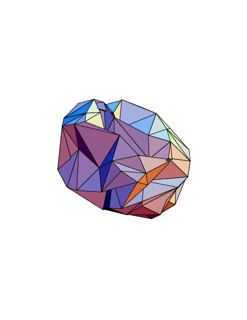
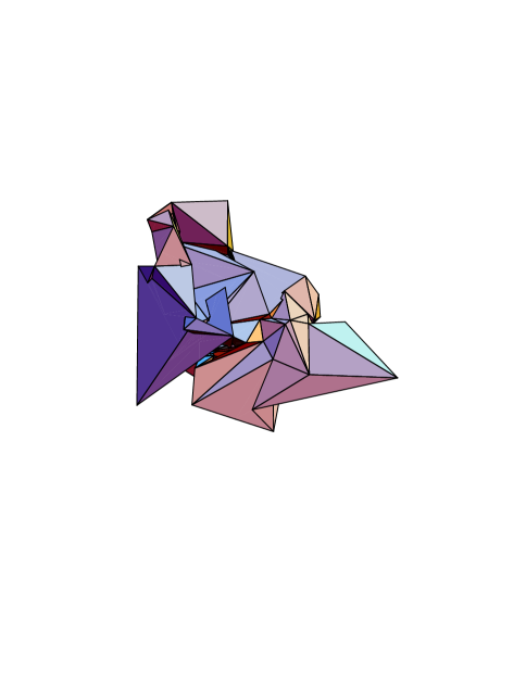
Figure 3: Equilibrium surfaces with the topology of a sphere, embedded in three dimensional flat space. The $R^{2}$ couplings are $\beta/A=0.5$ (left graph) and $\beta/A=0.0005$ (right graph). The number of triangles is $N_{2}=192$. In the left graph one vertex with coordination number four is visible.

Finally we have also constructed skeletons with $\chi=-2$, which have two handles. These skeletons are obtained by gluing together two tori of size $N^{2}$, as illustrated in fig. 2b. In both tori we cut out a square window of size $N/2$ and glue them together by identifying the links that are on the boundaries of the two windows. The four corner points in the window frame have a coordination number larger than six: two have coordination number eight and two have ten. All other vertices have coordination number six. The total number of vertices on such a bi-torus is $N_{0}=3N^{2}/2-2$ ($N$ must be even), the number or triangles is $N_{2}=2N_{0}+4$ and the number of links is $N_{1}=3N_{0}+6$.

5 Numerical results

In order to compute the string susceptibility and renormalized cosmological constant we have to compute the $A/\beta$ dependence of the average action in the constraint area model for $N_{2}\rightarrow\infty$. This term should behave as $(\beta/A)\langle\sum_{j}A_{j}\;\sum_{i}R_{i}^{2}\rangle=(A/\beta)\;\delta\lambda+\delta\gamma+O(\beta/A)$, which leads to the string susceptibility $\gamma_{{\rm str}}=\delta\gamma+2$, cf. eqs. (3.8) and (3.9) above.

Figure 4: Histograms for the bi-torus (fig. a), the sphere (fig. b) and the torus (fig. c). We have plotted $S_{R^{2}}(\beta/a)=\beta\mbox{$\langle\sum_{i}R_{i}^{2}/N_{2}\rangle$}_{A}$ as a function of $\beta/a$ for several lattices (bi-torus: from top to bottom $N_{2}=108,\ldots,1728$; sphere: from top to bottom $N_{2}=192,\ldots,4332$; torus: from bottom to top $N_{2}=18,\ldots,4608$). The circles represent the data points. We have dropped the error bars when they are smaller than the symbol size.

Most of our data have been generated with the unconstraint action. We used the histogramming method to compute the average action $\beta\langle\sum_{i}R_{i}^{2}\rangle_{A}$ with the constraint expectation value $\mbox{$\langle\bullet\rangle$}_{A}$ defined in eq. (4.2). For a fixed value of $\beta$ the distribution of triangle areas in an ensemble is peaked around an average triangle area $a\equiv\mbox{$\langle\sum_{i}A_{i}\rangle$}/N_{2}$, with $N_{2}$ the number of triangles in the skeleton. For increasing $N_{2}$ the peak of the distribution becomes more narrow, but remains roughly at the same value of $a$. In our numerical simulations we have kept $\beta$ fixed when increasing $N_{2}$. Eq. (4.3) shows that it then would require tuning $\beta\propto N_{2}$ to keep the bin with a fixed value of $\sum_{i}A_{i}/\beta$ sufficiently populated when increasing the skeleton size.

It requires several steps to estimate a value for the shift of the string susceptibility $\delta\gamma$: First we generate a large ensemble of $10^{5}-3\times 10^{5}$ configurations for each lattice size and store for each configuration the values of $\sum_{i}A_{i}$ and $\sum_{i}R^{2}_{i}$. Then we use the histogramming technique to compute the expectation value $S_{R^{2}}(\beta/a)\equiv\beta\mbox{$\langle\sum_{i}R_{i}^{2}/N_{2}\rangle$}_{A}$ for several values of the ratio $\beta/a$. In fig. 4 we have plotted $S_{R^{2}}(\beta/a)$ as a function of $\beta/a$ for skeletons with topologies of a bi-torus (fig. 4a), a sphere (fig. 4b) and a torus (fig. 4c). The circles indicate the centers of the bins. On the larger lattices the width of the distribution is substantially larger than the $\beta/a$ interval shown in fig. 4 and most of the data points are outside the frames. Each figure contains the results for a number of different lattice sizes. These distributions overlap over the full range of values of $N_{2}$ which makes it easy to read of the $N_{2}$ dependence. As noted above, this would not be the case if we would plot $S_{R^{2}}$ as a function of $\beta/\sum_{i}A_{i}$. The solid lines in figs. 4a, b, and c have been obtained by a polynomial fit which has been used to interpolate these results to obtain $S_{R^{2}}(\beta/a)$ over a range of $\beta/a$ values. The fits on the smaller lattices include also those data which are outside the frames.

In figs. 5a, b and c we have displayed the interpolated values for $S_{R^{2}}(\beta/a)$ as a function of $1/N_{2}$ for the three different topologies and several fixed values of $\beta/a$. It is seen that for the larger values of $N_{2}$ shown in the figure, the data fall nicely on straight lines. For smaller $N_{2}$ we find deviations from the straight line behavior. This shows that for sufficiently large $N_{2}$ $S_{R^{2}}(\beta/a)$ behaves as

$$S_{R^{2}}(\beta/a)=c_{0}(\beta/a)+c_{1}(\beta/a)/N_{2}+\cdots\;.$$ (5.1)

The coefficients $c_{0}$ and $c_{1}$ are found using a $\chi^{2}$ fit (straight lines in figs. 5a, b and c). The value of $\chi^{2}$ was in all cases smaller than two.

Next we have to convert the results for $c_{0}$ and $c_{1}$ into an estimate for the string susceptibility and the renormalized cosmological constant. In sect. 3 we have shown that,

$$\mbox{$\langle\beta\sum_{i}R^{2}\rangle$}_{A}=N_{2}\;S_{R^{2}}(N_{2}\beta/A)=N_{2}\;c_{0}(N_{2}\beta/A)+c_{1}(N_{2}\beta/A)+\cdots$$ (5.2)

should behave as, cf. eq. (3.8),

$$\mbox{$\langle\beta\sum_{i}R^{2}\rangle$}_{A}=-\frac{N_{1}\;\zeta}{2}-\frac{A}{\beta}\;\delta\lambda+\delta\gamma+O(\beta/A)\;.$$ (5.3)

This is the case if the coefficients $c_{0}$ and $c_{1}$ can be expanded as $c_{0,1}(x)=c_{0,1}^{(0)}+c_{0,1}^{(1)}/x+O(1/x^{2})$. Combining all results then leads to the relations

$$\delta\lambda=-c_{0}^{(1)}\;,\;\;\;\;\;\;\;\;\delta\gamma=c_{1}^{(0)}\;.$$ (5.4)

In order to cancel the term $\propto N_{1}$ in the right hand side of eq. (3.8), we should choose the measure such that

$$\zeta+4\;c_{0}^{(0)}/3=0\;.$$ (5.5)

Here we have used the relation $N_{1}/N_{2}=3/2$ which is valid for any two dimensional skeleton.

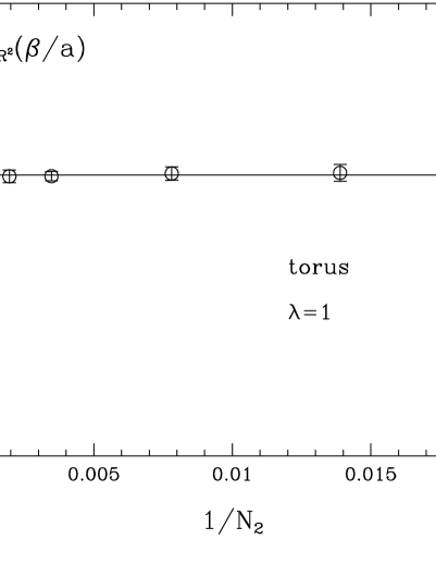
Figure 5: $S_{R^{2}}(\beta/a)=\beta\mbox{$\langle\sum_{i}R_{i}^{2}/N_{2}\rangle$}_{A}$ as a function of $1/N_{2}$ for the bi-torus (a), the sphere (b) and the torus (c). We have not included in these graphs the $S_{R^{2}}(\beta/a)$ results on small volumes since they exhibit deviations from the straight line behavior. The symbols and lines in figs. a-c correspond to various values of $\beta/a$: (a) $\Box:\beta/a=0.61$, ${\rm o}:\beta/a=2.4$, $\triangle:\beta/a=4.5$; (b) $\Box:\beta/a=0.61$, $\bullet:\beta/a=2.5$, $\triangle:\beta/a=4.5$; (c) $\triangle:\beta/a=2.4$. The full circles in fig. b have been generated with the Hybrid Monte Carlo algorithm. The straight lines have been obtained by fitting the numerical data to the ansatz (5.1).

In order to make contact with ref. [16], we have used the scale invariant measure, $\zeta=0$. Then relation (5.5) is not satisfied, but we shall nevertheless define a string susceptibility from the finite part of $\mbox{$\langle\sum_{i}R^{2}_{i}\rangle$}_{A}$, i.e. $\gamma_{{\rm str}}=c_{1}^{(0)}+2=c_{1}(\infty)+2$. We shall show below that $c_{1}^{(0)}$ in fact appears not to change much when tuning $\zeta$ such that (5.5) is fulfilled.

To determine this susceptibility from our numerical data we have to extrapolate the $c_{1}(\beta/a)$ data to $\beta/a=\infty$. The results for $c_{1}(\beta/a)$ are plotted in fig. 6 as a function of $\beta/a$ for the bi-torus (fig. a) and the sphere (fig. b). The two plots show that it is difficult to extrapolate reliably to large values of $\beta/a$. For the bi-torus we find from our data a lower limit $\delta\gamma=c_{1}^{(0)}\mbox{}_{\textstyle\sim}^{\textstyle>}3.5$, provided that $c_{1}(\beta/a)$ keeps monotonously increasing for $\beta/a>15$. Using the heuristic fit ansatz

$$c_{1}(x)=A+B/(x+C)$$ (5.6)

we find plausible values for $c_{1}^{(0)}$ in the range $4.0\stackrel{{\scriptstyle<}}{{\sim}}c_{1}^{(0)}\stackrel{{\scriptstyle<}}{{\sim}}5.0$. The curves obtained by fitting the $c_{1}(\beta/a)$ data to the ansatz (5.6) are represented in fig. 6 by the solid lines.

Figure 6: The coefficient $c_{1}(\beta/a)$ as a function of $\beta/a$ for the bi-torus (fig. a) and the sphere (fig. b). Most of the numerical results have been obtained with the histogramming method (open circles and triangle). The results represented in fig. b by the full circles have been obtained with the fixed area Hybrid Monte Carlo code. The full lines are fits with the heuristic ansatz (5.6). The fit in fig. a does not include the five points at $\beta/a\approx 0.20$. The dashed lines represent the $\gamma_{\rm str}-2$ values in the continuum. The triangle in fig. a has been obtained at $\beta/a=1.7$, $\zeta=-0.2$ which is closer to the point where (5.5) is fulfilled.

For the sphere we have computed $c_{1}(\beta/a)$ only for a few $\beta/a$ values. Fig. 6b shows that the $\beta/a$ dependence of the coefficient $c_{1}(\beta/a)$ is much weaker than for the bi-torus, but also in this case $c_{1}(\beta/a)$ appears to increase monotonously with $\beta/a$. The data which are represented by the full circles have been obtained with the fixed area Hybrid Monte Carlo code. We have used the generalized triangle inequalities which put a non-zero lower limit on the minimum triangle area ($\epsilon=0.01$), as discussed in sect. 4.2. As can be seen in fig. 6b, such a small value of $\epsilon$ appears not to lead to significant deviations compared with the Metropolis results. From this figure we can read of a lower bound for $c_{1}^{(0)}$ which is approximately equal to 3.5.

These results were obtained using the same scale invariant measure as in ref. [16]. It is clear that the resulting values for $\gamma_{{\rm str}}=2+c_{1}^{(0)}$ are in strong disagreement with the continuum predictions for both topologies: For the bi-torus we find $\gamma_{{\rm str}}\mbox{}_{\textstyle\sim}^{\textstyle>}5.5$ whereas the continuum value is $\gamma_{{\rm str}}=4.5$ and for the sphere we find $\gamma_{{\rm str}}\mbox{}_{\textstyle\sim}^{\textstyle>}5.5$ whereas the continuum value is $\gamma_{{\rm str}}=-0.5$. The continuum values of $\gamma_{{\rm str}}-2$ are represented in fig. 6a and b by the horizontal dashed lines. For the torus we find that $c_{1}(\beta/a)\approx 0$, independent of $\beta/a$ and hence also $\delta\gamma=c_{1}^{(0)}\approx 0$, as in the continuum. This means that the partition function obeys the scaling relation $Z(A)\propto A^{-1}$, which, as we pointed out in sect. 2.1, also holds for the classical model. Therefore it gives no information on the contribution of quantum effects, and finding the correct scaling of the Regge partition function for this case is of little significance.

The results for the bi-torus and sphere show that the claim of ref. [16], that the Regge model with a scale invariant measure reproduces the continuum values of the string susceptibility, is not justified. However, we have argued above that the value of $\zeta$ in the measure has to be chosen such that the term $\propto N_{1}$ in the expectation value of the action is canceled, cf. eq. (5.5). This is not the case when using the scale invariant measure: e.g. we find for the bi-torus $c_{0}(\beta/a)=0.1072(4)$, $0.1627(7)$, $0.2096(2)$, $0.2225(2)$, $0.2316(2)$, $0.2355(6)$ for $\beta/a=0.192$, $0.61$, $2.4$, $4.5$, $8.6$, $12.6$ and clearly (5.5) is not fulfilled since $\zeta=0$ in our case.

To check if the numerical results change when adjusting $\zeta$ such that $c_{0}+3\zeta/4$ becomes closer to zero, we have performed a simulation at $\beta=0.1$ and $\zeta=-0.2$ for the case of the bi-torus. For $\beta/a=1.7$ we find $c_{0}+3\zeta/4\approx 0.0904(4)$ which is indeed almost by a factor two smaller than the value of $c_{0}+3\zeta/4$ obtained for $\zeta=0$ at the same value of $\beta/a$. The result for the coefficient $c_{1}$ is represented in fig. 6a by the triangle. Even though the error bar is rather large, it occurs that the result falls on top of the fit curve to the $\zeta=0$ results which indicates that the coefficient $c_{1}(\beta/a)$ does not depend on the measure parameter $\zeta$.

6 Summary and final remarks

In this paper we have investigated the Regge method of regularizing the euclidean path integral for quantum gravity, using the two dimensional model as a test case. We have shown that a Regge skeleton can be viewed as a discretization of a smooth continuum manifold, which is defined by a metric field $g_{\mu\nu}$. The Regge action, including $R^{2}$ terms, approximates the corresponding continuum action, up to discretization errors. These discretization errors break diffeomorphism invariance, as illustrated in eq. (2.12) for the cosmological term in the action.

This suggests to separate the Regge degrees of freedom, the edge lengths of the skeleton, into equivalence classes, as in the continuum. We have given such a possible prescription in which skeletons are equivalent if they are related by a “gauge transformation” $l\rightarrow l^{\xi}$, cf. eq. (2.13). In a Gaussian approximation of the action around flat space, these transformations are zero modes, and correspond to the continuum gauge transformations [15]. The presense of these modes suggests that the measure in the Regge path integral should include a gauge fixing and Faddeev-Popov term, as in the continuum. However, it is not known how to implement this in practical simulations, and so far only simple variations on a scale invariant measure have been used.

Our numerical simulations have been done with such a simple measure. One can derive scaling relations for the Regge path integral of two dimensional $R^{2}$ gravity, which relates $d\log Z(A)/dA$ to the expectation value of the curvature square term, evaluated at a fixed value $A$ of the total area of the two dimensional surface [16]. We use two Monte Carlo methods to compute the constraint expectation values. In the first of these methods we simulate the unconstraint path integral and implement the fixed area constraint a posteriori by using a histogramming technique. The second method is a Hybrid Monte Carlo algorithm with which such a constraint model can be simulated directly. This algorithm is very attractive, because it can easily be vectorized and in comparison to the histogramming method it is more efficient because it allows us to carry out a simulation at a chosen value of $\beta/a$.

From the exact scaling relations for the Regge partition function we infer that the string susceptibility is determined from the part of $\beta\mbox{$\langle R^{2}\rangle$}_{A}+N_{1}\zeta/2$ that is finite after removing the regularization, i.e. for $N_{1}\rightarrow\infty$. The first term is the expectation value of the action at a fixed value of the area $A$ and $\zeta$ is the measure parameter. The identification of this finite part is however ambiguous and depends sensitively on the specific form of the measure used, as can be seen by shifting the measure parameter $\zeta\rightarrow\zeta+\zeta_{1}/N_{1}$. This is particularly clear for $\beta=0$, where we find the exact result $\gamma_{\rm str}=\zeta_{1}/2$.

These considerations cast serious doubts on the claim made in ref. [16] that the Regge model with scale invariant measure reproduces the continuum values of the string susceptibility. To settle this, we have also performed a numerical simulation of this model: as improvements over the earlier work, we have done the simulation at a fixed value of the total area, we have used a spherical topology with a more regular skeleton which only has coordination numbers four and six, and we also included a topology with genus $h=2$, the bi-torus. Otherwise we use the same scale invariant measure and $R^{2}$ term as in ref. [16]. We have determined the coefficient $c_{1}(\beta/a)$ of the $1/N_{2}$ term in the average action to a high accuracy for all three topologies and for several values of the coupling constant $\beta/a$.

In ref. [16] the coefficient $c_{1}$ was wrongly identified with the string susceptibility. It turns out that $c_{1}$ depends strongly on $\beta/a$ for the case of the bi-torus. For the sphere the $\beta/a$ dependence is much weaker (see fig. 6) and for the torus we find no $\beta/a$ dependence. We have argued that the determination of the string susceptibility requires that $\beta/a\rightarrow\infty$ and that $\zeta$ is tuned such that eq. (5.5) is satisfied. In our simulations we have followed ref. [16] and chosen the scale invariant measure $\zeta=0$, for which eq. (5.5) is not fulfilled. Simulations at a negative value of $\zeta$ at which this equality is almost satisfied indicate that $c_{1}$ is not affected by a small change in $\zeta$. Assuming that we do not include a term $\zeta_{1}/N_{1}$ in the measure, we can then from the $c_{1}(\beta/a)$ values shown in fig. 6 infer lower bounds on $\gamma_{\rm str}$. Both for the sphere and the bi-torus we find $\gamma_{{\rm str}}\mbox{}_{\textstyle\sim}^{\textstyle>}5.5$ which is substantially larger than the continuum values given in eq. (2.5). Only for the torus the string susceptibility reproduces the continuum value, but here the naive scaling holds, which does not involve quantum fluctuations.

A likely explanation for this failure of the Regge approach is the contribution of the gauge degrees of freedom, the $\xi$’s of eq. (2.13). These modes do not decouple form the action, because the Regge action is not gauge invariant (this is only approximately the case for small transformations of a smooth skeleton [15]). The gauge modes have also not been removed by including a gauge fixing and Faddeev-Popov term in the integration measure. If this is indeed the source of the failure of the Regge approach in two dimensional gravity, one would expect similar problems also in four dimensions.

To test this hypothesis and to improve the Regge approach, one could try to discretize the continuum model, including these gauge fixing and Faddeev-Popov terms. Such an approach faces many complications: The main obstacle is that one would have to find a practical method to simulate an action that includes such a gauge fixing term and Faddeev-Popov ghosts. Another serious complication arises from the breaking of the gauge (diffeomorphism) invariance which will produce gauge variant terms under renormalization. These terms have to be canceled by adding suitable counterterms. Furthermore, such gauge fixing and Faddeev-Popov ghost action expressed in terms of the Regge edge lengths, will be very cumbersome. Then it might be easier to abandon the Regge approach and use a more straightforward regularization of the path integral by discretizing the metric field $g_{\mu\nu}$ on a hypercubic lattice.

Acknowledgement

We have benefited from discussions with J. Kuti and C. Liu and thank them for many useful suggestions. Further we also like to thank W. Beirl, B. Berg, M. Golterman, U. Heller, J. Smit and M. Visser for useful discussions. This work was supported by the DOE under grant DE-FG03-91ER40546 and by the TNLRC under grant RGFY93-206. Some of the numerical simulations were done at the Livermore National Laboratory with DOE support for supercomputer resources and on the CRAY C90 at the San Diego Supercomputer Center.

References

-
[1]
J. Fröhlich, Lecture Notes in Physics,
Vol. 216, editor
L. Garrido, Springer (1985);
V.A. Kazakov, Phys. Lett. B150 (1985) 182. - [2] F. David, Nucl. Phys. B257 [FS14] (1985) 543.
- [3] T. Regge, Nuovo Cim. 19 (1961) 45.
- [4] H. Kawai, Nucl. Phys. B (Proc. Suppl.) 26 (1992) 93.
-
[5]
J.F. Wheater, Nucl. Phys. B (Proc. Suppl.) 34 (1994) 25;
J. Jurkiewicz, Nucl. Phys. B (Proc. Suppl.) 30 (1993) 108;
F. David, preprint SACLAY-T93-028, Lectures given at Les Houches Summer School on Gravitation and Quantizations, Session LVII, Les Houches, France, 1992;
J. Ambjrn, Nucl. Phys. B (Proc. Suppl.) 20 (1991) 701. - [6] L. Smolin, Nucl. Phys. B148 (1979) 333.
- [7] P. Menotti, Nucl. Phys. B (Proc. Suppl.) 17 (1990) 29 and further references therein.
-
[8]
H.W. Hamber and R.M. Williams, Nucl. Phys. B248 (1984) 392;
Phys. Lett. B157 (1985) 368; Nucl. Phys. B267 (1986) 482;
Nucl. Phys. B269 (1986) 712;
H.W. Hamber, in Critical Phenomena, Random Systems, Gauge Theories, Proceedings of the Les Houches Summer School, Session XLIII, edited by K. Osterwalder and R. Stora, Vol. 1 (North Holland, Amsterdam, 1986). -
[9]
J. Ambjrn, and J. Jurkiewicz,
Phys. Lett. B278 (1992) 42;
M.E. Agistein and A.A. Migdal, Mod. Phys. Lett A7 (1992) 1039; Nucl. Phys. B385 (1992) 395. - [10] J. Ambjrn, and J. Jurkiewicz, preprint NBI-HE-94-29 (hep-lat/9405010).
- [11] S. Catterall, J. Kogut and R. Renken, CERN preprint CERN-TH-7197-94, Illinois preprint ILL-TH-94-07 (hep-lat/9403019).
- [12] B.V. de Bakker and J. Smit, Amsterdam preprint ITFA-94-14 (hep-lat/9405013).
- [13] A. Nabutovsky and R. Ben-Av, Commn. Math. Phys. 157 (1993) 93.
- [14] J. Ambjrn, S. Jain and G. Thorleifsson, Phys. Lett. B307 (1993) 34.
- [15] M. Roček and R.M. Williams, Phys. Lett. B104 (1981) 31; Z. Phys. C21 (1984) 371.
- [16] M. Gross and H.W. Hamber, Nucl. Phys. B364 (1991) 703.
- [17] V.G. Knizhnik, A.M. Polyakov and A.B. Zamolodchikov, Mod. Phys. Lett. A3 (1988) 819.
- [18] F. David, Mod. Phys. Lett. A3 (1988) 1651.
- [19] J. Distler and H. Kawai, Nucl. Phys. B321 (1989) 509.
- [20] H. Kawai and R. Nakayama, Phys. Lett. B306 (1993) 224.
- [21] D.V. Boulatov, V.A. Kazakov, I.K. Kostov and A.A. Migdal, Nucl. Phys. B275 [FS17] (1986) 641.
- [22] K. Fujikawa, Nucl. Phys. B226 (1983) 437.
- [23] W. Bock, J. Smit and J.C. Vink, Nucl. Phys. B416 (1994) 645.
- [24] A. Borrelli, L. Maiani, G.C. Rossi, R. Sisto and M. Testa, Phys. Lett. B221 (1989) 360; Nucl. Phys. B333 (1990) 355.
- [25] W. Beirl, E. Gerstenmayer, H. Markum and J. Riedler, TU Vienna preprint (hep-lat/9402002).
- [26] B. Berg, Phys. Rev. Lett. 55 (1985) 904.
- [27] S. Duane, A.D. Kennedy, B.J. Pendelton and D. Roweth, Phys. Lett. B195 (1987) 216.