Radiative corrections to the kinetic couplings
in nonrelativistic lattice QCD

Abstract

The heavy-quark mass and wave function renormalizations, energy shift, and radiative corrections to two important couplings, the so-called kinetic couplings, in nonrelativistic lattice QCD are determined to leading order in tadpole-improved perturbation theory. The scales at which to evaluate the running QCD coupling for these quantities, except the wave function renormalization, are obtained using the Lepage-Mackenzie prescription. When the bare quark mass is greater than the inverse lattice spacing, the kinetic coupling corrections are roughly 10% of the tree-level coupling strengths; these corrections grow quickly as the bare quark mass becomes small. A need for computing the two-loop corrections to the energy shift and mass renormalization is demonstrated.

I Introduction

Nonrelativistic lattice QCD (NRQCD) is an effective field theory formulated to reproduce the action of continuum QCD at low energies [1, 2]. The NRQCD Lagrangian includes interactions which systematically correct for relativity and finite-lattice-spacing errors. To complete the formulation of NRQCD, the coupling strengths of its interactions must be determined. One possibility is to treat the couplings as adjustable parameters and tune them to fit certain experimental data; however, this tuning significantly reduces the predictive power of NRQCD simulations and is very costly and difficult. A better alternative is to compute the couplings in terms of the fundamental QCD coupling $\alpha_{s}=g^{2}/(4\pi)$ and the bare heavy-quark mass $M$ using perturbation theory. This is done by evaluating various scattering amplitudes in both QCD and lattice NRQCD and adjusting the couplings until these amplitudes agree at low energies. Since the role of these couplings is to compensate for neglected low-energy effects from highly-ultraviolet QCD processes, one expects that they may be computed to a good approximation using perturbation theory, provided that $a\Lambda_{\rm QCD}$ is small, where $a$ is the lattice spacing and $\Lambda_{\rm QCD}$ is the QCD scale parameter.

In this paper, the heavy-quark propagator in NRQCD is calculated to leading order in tadpole-improved perturbation theory and the on-mass-shell dispersion relation for the heavy quark is obtained. The mass renormalization, a shift in the zero point of energy, and the radiative corrections to the couplings of two important NRQCD interactions are determined by matching this dispersion relation to that of continuum QCD to $O(v^{4})$, where $v$ is the expectation value of the heavy-quark velocity in a typical heavy-quark hadron. The wave function renormalization is extracted from the on-shell residue of the perturbative propagator. These parameters are needed for high-precision numerical simulations of quarkonium and heavy-light mesons. Results are obtained using the standard Wilson action and a tree-level $O(a^{2})$-improved action for the gluons, and using two versions of the NRQCD action: one containing all $O(v^{2})$ spin-independent and all $O(v^{4})$ spin-dependent corrections to the leading kinetic term with tree-level removal of cutoff errors, the other including only $O(v^{2})$ corrections with no tree-level removal of lattice-spacing errors.

In addition, the scales at which to evaluate the running coupling for these quantities, except the wave function renormalization, are obtained for the first time using the Lepage-Mackenzie prescription. Choosing a value for $a\Lambda_{\rm QCD}$ from recent simulation measurements of the QCD coupling, numerical estimates of the energy shift, mass renormalization, and the radiative corrections to the two so-called kinetic couplings are also obtained. When $aM>1$, where $M$ is the bare quark mass, the radiative corrections to the kinetic couplings are roughly 10% of the tree-level coupling strengths; these corrections grow quickly as $aM$ becomes small. A range of estimates for the energy shift and mass renormalization are obtained after circumventing certain defects in the Lepage-Mackenzie prescription for setting the scale. The mass renormalization is small for $aM>3$ and becomes large as $aM$ decreases below this. Problems in reliably setting the scale result in large uncertainties in determining the energy shift and mass renormalization for small $aM$. These uncertainties underscore the need to compute the two-loop corrections to these renormalization parameters.

This work is partly an extension of previous calculations [3, 4] and is being carried out in conjunction with ongoing simulations as part of the NRQCD collaboration [5, 6].

The heavy-quark propagator in lattice NRQCD is briefly described in Sec. II. The energy shift, mass and wave function renormalizations, and the kinetic coupling corrections are defined and their calculation is outlined in Sec. III. The determination of the Lepage-Mackenzie scales is also described in this section. Results of these calculations are presented in Sec. IV. A final summary and suggestions for future work are given in Sec. V.

II Quark propagator in lattice NRQCD

The heavy-quark propagator ${\cal G}(x)=a^{3}\langle\psi(x)\psi^{\dagger}(0)\rangle$ in lattice NRQCD may be defined such that it satisfies an evolution equation given by [7]

$${\cal G}(x\!+\!a{\hat{e}}_{4}) = u_{0}^{-1}U^{\dagger}_{4}(x)\ [O(x){\cal G}(x)+\delta(x;0)],$$ (1)

$$O(x) = \Bigl{(}1\!-\!{aH_{0}\over 2n}\Bigr{)}^{n}\!(1\!-\!a\delta H)\Bigl{(}1\!-\!{aH_{0}\over 2n}\Bigr{)}^{n},$$ (2)

$${\cal G}(x) = 0,\quad\quad(x_{4}\leq 0)$$ (3)

where $a$ is the lattice spacing, $n$ is a positive integer[1], $\psi(x)$ is the heavy-quark field, $U_{\mu}(x)$ is the link variable representing the gauge field along the link between sites $x$ and $x+a{\hat{e}}_{\mu}$ with $({\hat{e}}_{\mu})_{\alpha}=\delta_{\mu\alpha}$, and $u_{0}$ is a mean-field parameter [8] defined in terms of the average plaquette. The nonrelativistic kinetic energy operator $H_{0}$ is given by

$$H_{0}=-{{\bf\Delta}^{(2)}\over 2M},$$ (4)

and the relativistic and finite-lattice-spacing corrections are included with coupling strengths $c_{j}$ in

$$\delta H=\sum_{j=1}^{8}c_{j}\ V_{j},$$ (5)

where

$$V_{1} = -{({\bf\Delta}^{(2)})^{2}\over 8M^{3}}\Bigl{(}1+\frac{Ma}{2n}\Bigr{)},$$ (6)

$$V_{2} = \frac{a^{2}{\bf\Delta}^{(4)}}{24M},$$ (7)

$$V_{3} = {ig\over 8M^{2}}\bigl{(}{\bf\Delta}^{(\pm)}\cdot{\bf E}-{\bf E}\cdot{\bf\Delta}^{(\pm)}\bigl{)},$$ (8)

$$V_{4} = -{g\over 8M^{2}}{\hbox{\boldmath$\sigma$}}\cdot{\bf(\tilde{\Delta}^{(\pm)}\times\tilde{E}-\tilde{E}\times\tilde{\Delta}^{(\pm)})},$$ (9)

$$V_{5} = -{g\over 2M}{\hbox{\boldmath$\sigma$}}\cdot{\bf\tilde{B}},$$ (10)

$$V_{6} = -{g\over 8M^{3}}\{{\bf\Delta}^{(2)},{\hbox{\boldmath$\sigma$}}\cdot{\bf B}\},$$ (11)

$$V_{7} = -{3g\over 64M^{4}}\{{\bf\Delta}^{(2)},{\hbox{\boldmath$\sigma$}}\cdot({\bf\Delta^{(\pm)}\!\times\!E\!-\!E\!\times\!\Delta^{(\pm)})}\},$$ (12)

$$V_{8} = -{ig^{2}\over 8M^{3}}{\hbox{\boldmath$\sigma$}}\cdot{\bf E\times E}.$$ (13)

The covariant, tadpole-improved difference operators are defined by

$$a\Delta_{\mu}^{(+)} = u_{0}^{-1}U_{\mu}-1,$$ (14)

$$a\Delta_{\mu}^{(-)} = 1-u_{0}^{-1}U^{\dagger}_{\mu},$$ (15)

$$\Delta^{(\pm)} = \frac{1}{2}(\Delta^{(+)}+\Delta^{(-)}),$$ (16)

$$a^{2m}{\bf\Delta}^{(2m)} = \sum_{k=1}^{3}\left(u_{0}^{-1}[U_{k}+U^{\dagger}_{k}]-2\right)^{m},$$ (17)

and $\bf E$ and $\bf B$ are the cloverleaf, mean-field-improved chromoelectric and chromomagnetic fields, respectively[9]. Tree-level removal of the leading cutoff errors in these operators [2] produces the operators $\bf\tilde{\Delta}^{(\pm)}$, ${\bf\tilde{\Delta}}^{(2)}$, $\bf\tilde{E}$, and $\bf\tilde{B}$. The components of $\sigma$ are the standard Pauli spin matrices. The parameter $n$ eliminates doublers and stabilizes the evolution of the quark Green’s function when $n\gtrsim 3/(Ma)$.

The coupling coefficients $c_{j}$ are functions of $g$ and $aM$ and are determined by matching low-energy scattering amplitudes in lattice NRQCD with those from continuum QCD, order-by-order in perturbation theory. At tree level, the values of these couplings are unity[2]. The $O(\alpha_{s})$ matching determines the radiative corrections to the $c_{j}$ couplings and may possibly require the introduction of additional $O(a^{2})$-suppressed interactions.

The operators $V_{1}$ and $V_{2}$, although appropriately gauged, will be referred to here as kinetic operators because they affect the energy of the free quark in the absence of the gluon fields. Their associated couplings $c_{1}$ and $c_{2}$ will be called kinetic couplings.

III Kinetic couplings and renormalizations

The kinetic couplings $c_{1}$ and $c_{2}$, the energy shift, and the heavy-quark mass and wave function renormalizations may be determined by studying the heavy-quark propagator in perturbation theory. An important consideration in the perturbative study of this propagator is the choice of expansion parameter. Lepage and Mackenzie have advocated a renormalized running QCD coupling defined in terms of the short-distance static-quark potential and evaluated at a prescribed mass scale. Their coupling shall be adopted here.

In this section, Eq. 1 is solved perturbatively to $O(\alpha_{s})$. The dispersion relation obtained from this solution is then matched to that of continuum QCD to $O(v^{4})$ to determine the heavy-quark mass renormalization, the shift in the zero point of energy, and the radiative corrections to $c_{1}$ and $c_{2}$. The wave function renormalization is then obtained from the on-shell residue of the perturbative propagator. Lastly, a brief description of the Lepage-Mackenzie coupling $\alpha_{V}(q^{\ast})$ is presented and their procedure of setting the scale $q^{\ast}$ is applied to the renormalization parameters and kinetic couplings.

A Heavy-quark self-energy

The heavy-quark self-energy $\Sigma(p)$ is defined by writing the full inverse quark propagator ${\cal G}^{-1}(p)$ in the form

$$a{\cal G}^{-1}(p)_{\alpha\beta}^{ij}=Q^{-1}(p)\delta^{ij}\delta_{\alpha\beta}-a\Sigma^{ij}_{\alpha\beta}(p),$$ (18)

where $i,j$ are color indices, $\alpha,\beta$ are spin indices, $p=({\bf p},p_{4})$ is a four-momentum in Euclidean space, and $Q(p)$ is the zeroth-order heavy-quark propagator in momentum space given by:

$$Q(p) = \Bigl{[}e^{ip_{4}a}-\Lambda_{n}({\bf p})\ \Gamma_{n}{(\bf p})^{2n}\Bigr{]}^{-1},$$ (19)

$$\Gamma_{n}({\bf p}) = 1-\frac{\kappa_{2}({\bf p})}{nMa},$$ (20)

$$\Lambda_{n}({\bf p}) = 1+{2\kappa_{2}({\bf p})^{2}\over M^{3}a^{3}}\Bigl{(}1+\frac{Ma}{2n}\Bigr{)}-{2\kappa_{4}({\bf p})\over 3Ma},$$ (21)

with $\kappa_{n}({\bf p})=\sum_{j=1}^{3}\sin^{n}\left(p_{j}a/2\right)$. At leading order in perturbation theory, this self-energy is given by:

$$\Sigma^{ij}_{\alpha\beta}(p)=\alpha_{s}\delta^{ij}\delta_{\alpha\beta}\biggl{[}\Sigma^{(A)}(p)\!+\!\Sigma^{(B)}(p)\!+\!\Sigma^{(C)}(p)\biggr{]},$$ (22)

where $\Sigma^{(A)}(p)$ denotes the contribution from the quark-gluon loop diagram shown in Fig. 1(A), $\Sigma^{(B)}(p)$ represents the contribution from the tadpole graph shown in Fig. 1(B), and $\Sigma^{(C)}(p)$ denotes the sum of the order $\alpha_{s}$ contributions from the $c_{1}$, $c_{2}$, and link-variable renormalization counterterms which arise when one writes $u_{0}=1+\alpha_{s}u_{0}^{(2)}+O(\alpha_{s}^{2})$ and $c_{j}=1+\alpha_{s}c_{j}^{(2)}+O(\alpha_{s}^{2})$.

The self-energy $\Sigma(p)$ is invariant under interchange of any two spatial momentum components $p_{i}\leftrightarrow p_{j}$ and under spatial momentum reflections $p_{j}\rightarrow-p_{j}$, and transforms into its complex conjugate under $p_{4}\rightarrow-p_{4}^{\ast}$. From these properties, the small-${\bf p}$ representation of the self-energy may be written:

$$a\Sigma(p) \approx \alpha_{s}\Bigl{\{}f_{0}(w)+f_{1}(w){{\bf p}^{2}a^{2}\over 2Ma}+f_{2}(w)\frac{({\bf p}^{2})^{2}a^{4}}{8M^{2}a^{2}}$$ (23)

$$+ f_{3}(w)\ (\sum_{j=1}^{3}p_{j}^{4}a^{4})+\dots\Bigr{\}},$$ (24)

where $w=-ip_{4}a$. When $w$ is small, the functions $f_{m}(w)$ are represented well by their power series expansions $f_{m}(w)=\sum_{l=0}^{\infty}\Omega_{m}^{(l)}\ w^{l}$.

The moments $\Omega_{m}^{(l)}$ are obtained from integrals of the form

$$\Omega_{m}^{(l)}=\int_{-\pi/a}^{\pi/a}\frac{d^{4}q}{(2\pi)^{4}}\ \xi_{m}^{(l)}(q),$$ (25)

where $q$ is the momentum of the gluon in the loop diagrams shown in Fig. 1 and $\xi_{m}^{(l)}(q)$ is some combination of vertex factors and Feynman propagators. To evaluate these integrals [10], first, a small gluon mass $\lambda$ is introduced to provide an infrared cutoff. Due to singularities in the integrands from the zeroth-order quark propagator, it is best to first evaluate the integrals over the temporal component of $q$ analytically. Using $z=\exp(-iq_{4}a)$, the $q_{4}$ integrations are transformed into contour integrals along the $|z|=1$ unit circle which can be evaluated by the residue theory. The remaining integrals over the spatial components of $q$ are then approximated numerically by discrete sums using $aq_{j}=2\pi n_{j}/N$, where the $n_{j}$ take all integer values satisfying $-N/2<n_{j}\leq N/2$ for integral $N$. The error made in this approximation diminishes exponentially fast as $N\rightarrow\infty$, but the rate of decay is proportional to $\lambda$. Convergence in $N$ can be dramatically improved by making the following change in the variables: $q_{j}\rightarrow q_{j}-\alpha\sin q_{j}$, where $\alpha={\rm sech}u$ and $u$ satisfies $a\lambda=u-{\rm tanh}u$. Extrapolation of the results to zero gluon mass is accomplished using a least-squares fit to the form: $\sum_{m=0}^{N}b_{m}^{(0)}(a\lambda)^{m}+\sum_{m=1}^{M}b_{m}^{(1)}(a\lambda)^{m}\ln a^{2}\lambda^{2}$. Calculations are performed in the Feynman gauge.

The contributions from $\Sigma^{C}(p)$ to the $f_{m}(w)$ functions appearing in Eq. 23 can be exactly determined. One finds

$$f_{0}^{(C)}(w) = -u_{0}^{(2)}\biggl{(}e^{-w}\!+\!\frac{3}{Ma}\biggr{)},$$ (26)

$$f_{1}^{(C)}(w) = \frac{2}{3}u_{0}^{(2)}\biggl{(}1\!+\!\frac{9}{2Ma}\!+\!\frac{9}{2M^{2}a^{2}}\biggr{)},$$ (27)

$$f_{2}^{(C)}(w) = -\frac{4}{3}u_{0}^{(2)}\biggl{(}1\!+\!\frac{3}{8Ma}\Bigl{(}10\!+\!\frac{3}{n^{2}}\Bigr{)}\!+\!\frac{27}{4M^{2}a^{2}}\biggr{)}$$ (28)

$$+ c_{1}^{(2)}\biggl{(}\frac{1}{2n}\!+\!\frac{1}{Ma}\biggr{)},$$ (29)

$$f_{3}^{(C)}(w) = \frac{u_{0}^{(2)}}{18Ma}\biggl{(}1\!-\!\frac{9}{4M^{2}a^{2}}\biggr{)}\!-\!\frac{c_{2}^{(2)}}{24Ma}.$$ (30)

Contributions to the moments $\Omega_{m}^{(l)}$ from the $c_{1}$, $c_{2}$, and mean-field improvement counterterms in $\Sigma^{(C)}(p)$ are then easily determined from the power series expansions of these functions.

B Matching

From the heavy-quark propagator computed to $O(\alpha_{s})$ in perturbation theory, one finds that the on-mass-shell quark satisfies a dispersion relation given to order $v^{4}$ by

$$\omega_{0}({\bf p})\approx{{\bf p}^{2}\over 2M_{r}}-{({\bf p}^{2})^{2}\over 8M_{r}^{3}}-\alpha_{s}\delta\omega({\bf p})+\dots,$$ (31)

where $\omega_{0}({\bf p})$ is the value of $w=-ip_{4}a$ at which the inverse propagator vanishes, $M_{r}$ is the renormalized mass given by $M_{r}=Z_{m}M$ with $Z_{m}=1+\alpha_{s}(\Omega_{0}^{(0)}+\Omega_{0}^{(1)}+\Omega_{1}^{(0)})$, and

$$a\delta\omega({\bf p}) = W_{0}+W_{1}\ \frac{({\bf p}^{2})^{2}a^{4}}{8M^{2}a^{2}}+W_{2}\ (\sum_{j=1}^{3}p_{j}^{4}a^{4}),$$ (32)

$$W_{0} = \Omega_{0}^{(0)},$$ (33)

$$W_{1} = \Omega_{0}^{(0)}\left(1+\frac{2}{Ma}\right)+2\Omega_{0}^{(1)}\left(1+\frac{1}{Ma}\right)+2\Omega_{0}^{(2)}$$ (34)

$$+ \Omega_{1}^{(0)}\left(2+\frac{3}{Ma}\right)+2\Omega_{1}^{(1)}+\Omega_{2}^{(0)},$$ (35)

$$W_{2} = \Omega_{3}^{(0)}.$$ (36)

Note that the rest mass $M_{r}$ has been removed from the heavy-quark energy in Eq. 31.

The order $\alpha_{s}$ corrections to the heavy-quark propagator in QCD only renormalize the quark field and mass to order $v^{4}$ so that the dispersion relation for the quark in continuum QCD is given by

$$\omega_{\rm QCD}({\bf p})\approx{{\bf p}^{2}\over 2M_{r}}-{({\bf p}^{2})^{2}\over 8M_{r}^{3}}+\dots\ .$$ (37)

If lattice NRQCD is to reproduce the low-energy physical predictions of full QCD, then $\delta\omega({\bf p})=0$ is required in Eq. 31; that is, $W_{0}=W_{1}=W_{2}=0$. Alternatively, since the constant term $W_{0}$ represents an overall energy shift, one could require only $W_{1}=W_{2}=0$ and then simply shift the energies obtained in simulations by an amount $\alpha_{s}W_{0}/a+M_{r}$ for each heavy quark. Setting $W_{1}=W_{2}=0$ determines the coefficients $c_{1}^{(2)}$ and $c_{2}^{(2)}$, and defining $\bar{p}_{4}=p_{4}+i\alpha_{s}W_{0}/a$, the inverse propagator for small $v$ may then be written:

$$a{\cal G}^{-1}(p)\approx Z_{\psi}^{-1}\left(i\bar{p}_{4}a+{{\bf p}^{2}a^{2}\over 2M_{r}a}+\dots\right),$$ (38)

where $Z_{\psi}=1-\alpha_{s}(\Omega_{0}^{(0)}+\Omega_{0}^{(1)})+O(v^{2},\alpha_{s}v^{2})$ is the wave function renormalization.

A more convenient set of renormalization parameters may be obtained by defining

$$\bar{p}_{4} = p_{4}-i\alpha_{s}A/a,$$ (39)

$$Z_{m} = 1+\alpha_{s}B,$$ (40)

$$Z_{\psi} = 1+\alpha_{s}(C+C_{\rm div}),$$ (41)

where $C_{\rm div}=-2(\ln a^{2}\lambda^{2})/(3\pi)$ is the infrared-divergent portion of the wave function renormalization. The parameters $A$, $B$, and $C$ can then be calculated using $A=-\Omega_{0}^{(0)}$, $B=\Omega_{0}^{(0)}+\Omega_{0}^{(1)}+\Omega_{1}^{(0)}$, and $C=-(\Omega_{0}^{(0)}+\Omega_{0}^{(1)}+C_{\rm div})$.

C Expansion parameter $\alpha_{V}(q^{\ast})$

In order to obtain numerical values for the renormalization parameters and the kinetic couplings, one must determine the value of the renormalized QCD coupling $\alpha_{s}$. This can be done only after a definition of the running coupling and a procedure for determining the relevant mass scale are specified.

A renormalization scheme, due to Lepage and Mackenzie[8], which defines the coupling such that the short-distance static-quark potential has no $\alpha_{s}^{2}$ or higher-order corrections is particularly attractive. By absorbing higher-order contributions to the static-quark potential into the coupling, it is hoped that higher-order contributions to other physical quantities in terms of this coupling will then be small. In this scheme, the running coupling $\alpha_{V}(q)$ is defined by

$$V(q)\equiv-\frac{4\pi C_{F}}{q^{2}}\alpha_{V}(q)$$ (42)

for large $q$, where $C_{F}=4/3$ is the quark’s color Casimir and $V(q)$ is the static-quark potential at momentum transfer $q$. For sufficiently large $q$, this coupling runs according to the usual two-loop relation

$$\alpha_{V}(q)=\left[\beta_{0}\ln(q^{2}/\Lambda_{V}^{2})+\frac{\beta_{1}}{\beta_{0}}\ln\ln(q^{2}/\Lambda_{V}^{2})\right]^{-1},$$ (43)

where $\beta_{0}=(11-\frac{2}{3}N_{F})/(4\pi)$, $\beta_{1}=(102-\frac{38}{3}N_{F})/(16\pi^{2})$, $\Lambda_{V}$ is the QCD scale parameter, and $N_{F}$ is the number of dynamical quark flavors at mass scale $q$.

Lepage and Mackenzie have also devised a simple procedure for determining the scale $q^{\ast}$ at which to evaluate the coupling $\alpha_{V}(q^{\ast})$ for a given one-loop process [8]. For a one-loop perturbative contribution of the form

$$I_{\xi}=\alpha_{V}(q^{\ast})\int\frac{d^{4}q}{(2\pi)^{4}}\ \xi(q),$$ (44)

where $q$ is the momentum of the exchanged gluon, they suggest

$$\ln(q^{\ast 2})\equiv\frac{\int d^{4}q\ln(q^{2})\ \xi(q)}{\int d^{4}q\ \xi(q)}.$$ (45)

Clearly, difficulties with this definition will arise when $\int d^{4}q\ \xi(q)\sim 0$. Also note that the mean value theorem guarantees that $q^{\ast}$ will satisfy $0\leq aq^{\ast}\leq 2\pi$ only if $\xi(q)\geq 0$ for all $q$ throughout the region of integration $-\pi\leq aq_{\mu}\leq\pi$ (or $\xi(q)\leq 0$ for all such $q$).

To evaluate the scales $q^{\ast}_{A}$, $q^{\ast}_{B}$, $q^{\ast}_{c_{1}^{(2)}}$, and $q^{\ast}_{c_{2}^{(2)}}$ corresponding to the gauge-invariant quantities $A$, $B$, $c_{1}^{(2)}$, and $c_{2}^{(2)}$, respectively, integrals of the form

$$\hat{\Omega}_{m}^{(l)}=\int\frac{d^{4}q}{(2\pi)^{4}}\ \ln(q^{2})\ \xi_{m}^{(l)}(q),$$ (46)

must be calculated (recall Eq. 25). First, a small gluon mass $\lambda$ is introduced to circumvent infrared difficulties. Next, the $\ln(a^{2}q^{2})$ factor is approximated by $\ln\{\zeta(z)+a^{2}({\bf q}^{2}+\lambda^{2})\}$, where

$$\zeta(z)=-15\ \frac{31z^{4}+128z^{3}-318z^{2}+128z+31}{23z^{4}+688z^{3}+2358z^{2}+688z+23},$$ (47)

and $z=\exp(-iq_{4}a)$. Eq. 47 is simply a $[2/2]$ Pade approximant of $a^{2}q_{4}^{2}$ in terms of $\cos(aq_{4})$. This introduces a small error in the determination of the scale, but enables an analytical treatment of the integration over the temporal component of $q$. Singularities in the integrands make such a treatment crucial to reliably and efficiently evaluating these integrals. The remaining integrations over the spatial components of $q$ are then approximated numerically by discrete sums, as described previously in Sec. III A, and the $\lambda\rightarrow 0$ limits are finally taken.

IV Results and discussion

Results for $A$, $B$, $C$, $c_{1}^{(2)}$, $c_{2}^{(2)}$ and the scales $q^{\ast}_{A}$, $q^{\ast}_{B}$, $q^{\ast}_{c_{1}^{(2)}}$, $q^{\ast}_{c_{2}^{(2)}}$ are presented in this section. Since the wave function renormalization is not a gauge-invariant quantity, the scale corresponding to $C$ will not be considered here. Choosing a value for $a\Lambda_{V}$ from recent simulation measurements of $\alpha_{V}$, numerical estimates of the energy shift, mass renormalization, and the radiative corrections to the kinetic couplings are also obtained.

A Perturbative coefficients

Values for $A$, $B$, $C$, $c_{1}^{(2)}$, and $c_{2}^{(2)}$ have been determined for a large range of bare quark masses and for various values of the stability parameter $n$. Results were obtained using the standard Wilson action $S_{G}^{(W)}$ for the gluons and a tree-level $O(a^{2})$-improved gluonic action $S_{G}^{(I)}$ [2]. In addition, two versions of the NRQCD interaction operator $\delta H$ were used: one, denoted by $\delta H^{(4)}$, containing the full set of interactions $V_{1}-V_{8}$ in $\delta H$ (see Eqs. 5$-$13); the other, denoted by $\delta H^{(2)}$, including only the $O(v^{2})$ corrections $V_{1}-V_{5}$ with no tree-level removal of the cutoff errors in $V_{4}$ and $V_{5}$ (Eqs. 9 and 10 with the tildes removed). Contributions to these parameters from the tadpole-improvement counterterm are given by

$$\delta A = u_{0}^{(2)}\left(1+\frac{3}{Ma}\right),$$ (48)

$$\delta B = u_{0}^{(2)}\left(\frac{2}{3}+\frac{3}{M^{2}a^{2}}\right),$$ (49)

$$\delta C = u_{0}^{(2)}\frac{3}{Ma},$$ (50)

$$\delta c_{1}^{(2)} = \frac{u_{0}^{(2)}}{Ma+2n}\left(\frac{3}{n}-\frac{18n}{M^{2}a^{2}}\right),$$ (51)

$$\delta c_{2}^{(2)} = \frac{4}{3}u_{0}^{(2)}\left(1-\frac{9}{4M^{2}a^{2}}\right).$$ (52)

The mean-field correction is $u_{0}^{(2)}=-\epsilon\pi/3$, where $\epsilon=1$ for the simple gluonic action and $\epsilon=0.78463$ for the improved gluonic action.

The shift $A$ in the zero point of energy, the mass renormalization $B$, and the kinetic coupling corrections $c_{1}^{(2)}$ and $c_{2}^{(2)}$ before tadpole improvement $(u_{0}^{(2)}=0)$ are shown in Figs. 2 and 3 for the simple Wilson gluonic action $S_{G}^{(W)}$ and the $O(v^{2})$ version $\delta H^{(2)}$ of NRQCD [11]. Their values after tadpole improvement are shown in Figs. 4 and 5. These quantities are gauge invariant and infrared finite. In order to demonstrate the sensitivity of the tadpole-improved quantities to the form of the gluon action and the higher-order NRQCD interactions, results for $B$ after tadpole improvement using both versions $\delta H^{(2)}$ and $\delta H^{(4)}$ of NRQCD and the simple Wilson $S_{G}^{(W)}$ and the $O(a^{2})$-improved $S_{G}^{(I)}$ gluonic actions are shown in Fig. 6. The wave function renormalization parameter $C$ before and after mean-field improvement for $S_{G}^{(W)}$ and $\delta H^{(2)}$ is presented in Fig. 7.

Before tadpole improvement, these parameters are all very large, especially as $aM$ decreases. Tadpole contributions dominate and contain power-law divergences which grow as $aM$ becomes small. Since high-momentum modes are more strongly damped in the improved gluon propagator, the ultraviolet-divergent tadpole terms, and hence the couplings and renormalization parameters before tadpole improvement, are smaller in the case of the improved gluon action.

Mean-field improvement greatly reduces the magnitudes of all of these coefficients. For $aM>5$, $A$ is almost independent of $aM$ after tadpole improvement, with values near unity; as $aM$ decreases below $5$, $A$ also decreases, eventually changing in sign. After tadpole improvement, $B$ has a small negative value at large $aM$; as $aM$ decreases, $B$ increases, becoming positive, reaches a maximum near $aM\sim 1$, then rapidly decreases, eventually falling below zero again. The kinetic coupling coefficients $c_{1}^{(2)}$ and $c_{2}^{(2)}$ vary slowly for $aM\gtrsim 3/2$, then rise sharply as $aM$ decreases below this. $C$ also varies slowly, remaining a small correction, for $aM\gtrsim 3/2$ after mean-field improvement. As $aM$ decreases below unity, however, $C$ begins to grow quickly in magnitude. For large $aM$, these tadpole-improved parameters are only slightly sensitive to the value of $n$, the spin-dependent interactions, the cutoff improvement of the gluon action, and the $O(v^{4})$ relativity corrections of NRQCD (see Fig. 6). As $aM$ decreases, however, sensitivity to these factors grows. The kinetic couplings are generally more sensitive to these effects than are the renormalization parameters $A$, $B$, and $C$. The mass renormalization parameter $B$ is also very sensitive to the leading kinetic interactions $V_{1}$ and $V_{2}$.

B Scale determinations

The scales before tadpole improvement $(u_{0}^{(2)}=0)$ are shown in Figs. 8 and 9 for the simple Wilson gluonic action $S_{G}^{(W)}$ and the $O(v^{2})$ version $\delta H^{(2)}$ of NRQCD [11]. Their values after mean-field improvement are shown in Figs. 10 and 11. The qualitative behavior of these scales are not affected by the cutoff improvement of the gluon action and the $O(v^{4})$ relativity corrections of NRQCD. For large $aM$, the tadpole-improved scales are especially insensitive to these factors. As $aM$ decreases, however, quantitative sensitivity grows, becoming rather pronounced for $q^{\ast}_{c_{1}^{(2)}}$ and $q^{\ast}_{c_{2}^{(2)}}$.

Before tadpole improvement, the scales $q_{A}^{\ast}$ and $q_{B}^{\ast}$ are slowly varying functions of $aM$ for $aM<5$, ranging between $2/a$ and $3/a$ in value. As $aM$ becomes large, $q_{A}^{\ast}$ falls slowly to a value just below $2/a$, while $q_{B}^{\ast}$ rises to a value above $5/a$. Since the unimproved parameters are dominated by highly-ultraviolet tadpole contributions, scales in the range $2/a$ to $3/a$ are not surprising. The greater damping of the high-momentum modes in the case of the improved gluon action $S_{G}^{(I)}$ results in slightly lower scales in comparison to those obtained using the Wilson action.

The scales $q_{c_{1}^{(2)}}^{\ast}$ and $q_{c_{2}^{(2)}}^{\ast}$ also vary slowly between $2/a$ and $3/a$, except in the regions where the perturbative coefficients $c_{1}^{(2)}$ and $c_{2}^{(2)}$ are nearly zero. As these zeros are approached from below, the scales tend asymptotically to infinity; approached from above, the scales tend to zero. This dramatic behavior is an inevitable consequence of using Eq. 45 to define the scale and does not stem from any physical effect; whenever any perturbative coefficient nears zero, similar pathological behavior will be observed in the corresponding scale. Such points at which the scales tend to zero on one side and asymptotically to infinity on the other shall be referred to here as defects.

For $aM>3$, the scale $q_{A}^{\ast}$ is almost independent of $aM$ with values near $0.8/a$ after mean-field improvement, revealing a significant reduction from the tadpole removal. As $aM$ decreases below $3$, $q_{A}^{\ast}$ falls, becoming small as the zero in $A$ near $aM\sim 0.6$ is approached. For $aM$ below this zero, $q_{A}^{\ast}$ assumes large defective values which cannot be shown in Fig. 10. The mass renormalization scale $q_{B}^{\ast}$ becomes small as the zero in $B$ near $aM\sim 0.5$ is approached from above and the zero near $aM\sim 5$ is approached from below; it becomes infinitely large as one approaches these zeros from the opposite directions. Between these defects, $q_{B}^{\ast}$ attains a maximum value of only about $0.6/a$, and as $aM$ becomes large, $q_{B}^{\ast}$ tends to a value near $2/a$; both of these facts indicate a substantial lowering of $q_{B}^{\ast}$ from tadpole improvement.

For $aM>3$, the scale $q_{c_{2}^{(2)}}^{\ast}$ is significantly smaller after mean-field improvement and varies little; as $aM$ decreases below $3$, $q_{c_{2}^{(2)}}^{\ast}$ grows quickly, eventually reaching values above $6/a$, indicating an enhancement from tadpole removal. Note that mean-field improvement has eliminated all pathological values. $q_{c_{1}^{(2)}}^{\ast}$ displays behavior similar to that of $q_{c_{2}^{(2)}}^{\ast}$, except that $q_{c_{1}^{(2)}}^{\ast}$ grows to much greater values as $aM$ decreases, exceeding $15/a$ near $aM\sim 1$ before leveling off. These high values are a result of large, nearly canceling contributions in the loop integrals in Eq. 45.

C Size of the corrections

In addition to the perturbative coefficients $A$, $B$, $c_{1}^{(2)}$, $c_{2}^{(2)}$, and their associated scales, the QCD scale parameter $a\Lambda_{V}$ must be known before numerical estimates of the first-order energy shift $aE_{0}=A\ \alpha_{V}(q^{\ast}_{A})$, the mass renormalization $Z_{m}-1=B\ \alpha_{V}(q_{B}^{\ast})$, and the radiative corrections $\delta c_{1}=c_{1}^{(2)}\ \alpha_{V}(q^{\ast}_{c_{1}^{(2)}})$ and $\delta c_{2}=c_{2}^{(2)}\ \alpha_{V}(q^{\ast}_{c_{2}^{(2)}})$ can be determined. The most straightforward procedure for measuring $a\Lambda_{V}$ is to extract $\alpha_{V}(\mu)$ at some scale $\mu$ from simulations. One possibility is to fit simulation measurements of the logarithm of the mean plaquette to its perturbative expansion. Doing this, Lepage and Mackenzie [8] have extracted $\alpha_{V}(3.40/a)$ from Monte Carlo data for quenched QCD at several values of $\beta$, where $\beta=6/g^{2}$. At $\beta=6$, they find $\alpha_{V}(3.40/a)=0.152$, corresponding to $a\Lambda_{V}=0.169$ in Eq. 43; at $\beta=6.4$, they obtain $\alpha_{V}(3.40/a)=0.130$, yielding $a\Lambda_{V}=0.097$.

The leading-order radiative corrections $\delta c_{1}$ and $\delta c_{2}$ to the kinetic couplings are shown in Fig. 12 for $a\Lambda_{V}=0.169$ and using $\delta H^{(2)}$ and $S_{G}^{(W)}$. For $aM>1$, $\delta c_{1}$ and $\delta c_{2}$ are nearly independent of $aM$ and adjust $c_{1}$ and $c_{2}$ above their tree-level strengths by about 10%, a small amount. For $aM<1$, these corrections grow rapidly as $aM$ decreases, indicating the insufficiency of tree-level values for $c_{1}$ and $c_{2}$ as $aM$ becomes small. These large corrections also suggest that the NRQCD approach should be applied cautiously as $aM$ falls below unity.

The defects in $q^{\ast}_{A}$ and $q^{\ast}_{B}$ make determination of $aE_{0}$ and $Z_{m}-1$ problematical. One cannot simply use $aE_{0}=A\ \alpha_{V}(q^{\ast}_{A})$ and $Z_{m}-1=B\ \alpha_{V}(q^{\ast}_{B})$ near the defects since $\alpha_{V}(q)$ is not reliably known for $q$ below and near $\Lambda_{V}$. Imposing minimum and maximum scales also does not work since this produces large, unphysical discontinuities in $aE_{0}$ and $Z_{m}-1$ on crossing the defects. The $q^{\ast}$ prescription of Eq. 45 fails near the defects and it would seem that one must resort to guessing the appropriate scale. One suggestion for doing this is to inspect the scale plots and somehow smooth out the scales across the defects. However chosen, denote this guessed scale by $\bar{q}$ to distinguish it from the Lepage-Mackenzie scale $q^{\ast}$. Estimates of $aE_{0}$ and $Z_{m}-1$ can then be obtained by replacing $\alpha_{V}(q^{\ast})$ by $\alpha_{V}(\bar{q})$. A better procedure, however, is to replace $\alpha_{V}(q^{\ast})$ by its expansion in terms of the coupling renormalized at $\bar{q}$, namely,

$$\bar{\alpha}_{V}(q^{\ast};\bar{q})=\alpha_{V}(\bar{q})\left[1-\beta_{0}\ln\left(q^{\ast 2}/\bar{q}^{2}\right)\alpha_{V}(\bar{q})\right].$$ (53)

This incorporates information contained in $q^{\ast}$, yet yields results which are continuous across the defects.

A range of estimates for the energy shift $aE_{0}$ and mass renormalization $Z_{m}-1$ using Eq. 53 are presented in Fig. 13. Energy shift estimates $A\ \bar{\alpha}_{V}(q^{\ast}_{A};\bar{q}_{A})$ are shown choosing $\bar{q}_{A}=0.8/a$ and $0.6/a$ for all $aM$ values and using $a\Lambda_{V}=0.169$ in $\alpha_{V}(\bar{q}_{A})$. Mass renormalization estimates $B\ \bar{\alpha}_{V}(q^{\ast}_{B};\bar{q}_{B})$ are shown for the choices $\bar{q}_{B}=1.0/a$ and $0.6/a$ for all $aM$. These choices for $\bar{q}_{A}$ and $\bar{q}_{B}$ are based on an examination of the scales in Figs. 10 and 11. The energy shift $aE_{0}$ is remarkably independent of $aM$, in contrast to the perturbative coefficient $A$ which falls to below zero as $aM$ decreases. Sensitivity to the choice of $\bar{q}_{A}$ grows as $aM$ decreases. The mass renormalization is very small for $aM>3$ and is only mildly sensitive to the choice of $\bar{q}_{B}$; $Z_{m}-1$ becomes zero near where the perturbative coefficient $B$ vanishes. As $aM$ decreases below this, however, $Z_{m}-1$ grows quickly and continues to grow even after $B$ has fallen to below zero. As $aM$ becomes small, estimates of the mass renormalization become very large and the sensitivity of these estimates to $\bar{q}_{B}$ becomes pronounced. Both of these facts and the sensitivity of the energy shift to $\bar{q}_{A}$ for small $aM$ underscore the need to compute the two-loop corrections to $Z_{m}-1$ and $aE_{0}$.

V Conclusion

The heavy-quark propagator in NRQCD was calculated to $O(\alpha_{s})$ in tadpole-improved perturbation theory. The mass renormalization, shift in the zero point of energy, and the radiative corrections to the two kinetic couplings $c_{1}$ and $c_{2}$ were determined by matching the on-mass-shell dispersion relation for the heavy quark obtained from the NRQCD quark propagator to that of continuum QCD to $O(v^{4})$. In addition, the scales at which to evaluate the running coupling for these quantities were obtained for the first time using the Lepage-Mackenzie prescription. Defects in these scales were found. The wave function renormalization was extracted from the on-shell residue of the perturbative propagator. Results were obtained using two different gluon actions $S_{G}^{(W)}$ and $S_{G}^{(I)}$ and two versions of NRQCD, $\delta H^{(2)}$ and $\delta H^{(4)}$, differing only in the order of the relativity and finite-lattice-spacing corrections retained.

Using a typical value for $a\Lambda_{\rm QCD}$ from recent simulation measurements of $\alpha_{s}$, numerical estimates of the energy shift, mass renormalization, and the radiative corrections to $c_{1}$ and $c_{2}$ were also obtained. The radiative corrections to the kinetic couplings were found to be small for $aM>1$, being roughly 10% of the tree-level coupling strengths, and to grow quickly as $aM$ decreased below unity. Problems in reliably setting the scale complicated the determinations of the energy shift and mass renormalization for some values of $aM$. A simple modification of the running coupling was necessary to obtain a range of estimates for these parameters near these $aM$ values. The mass renormalization was found to be small for $aM>3$ and to become large as $aM$ decreased. Large uncertainties in determining the energy shift and mass renormalization for small $aM$ demonstrated the need to compute the two-loop corrections to these quantities.

Future work includes the evaluation of the other NRQCD couplings and the two-loop contributions to the mass renormalization and the energy shift. Computation of the couplings $c_{3}-c_{7}$ has already begun.

FIG. 1.: Two Feynman diagrams which contribute to the heavy-quark self-energy. A curly line denotes a gluon; a double solid line denotes a heavy quark.

FIG. 2.: The energy shift parameter $A$, heavy-quark mass renormalization parameter $B$, and the kinetic coupling coefficients $c_{1}^{(2)}$ and $c_{2}^{(2)}$ before tadpole improvement ($u_{0}=1$) against the product of the bare heavy-quark mass $M$ and the lattice spacing $a$ using $S_{G}^{(W)}$ and $\delta H^{(2)}$. The dot-dashed curve is $A$, the solid curve shows $B$, the dashed curve is $c_{1}^{(2)}$, and the dotted curve indicates $c_{2}^{(2)}$. For $aM>3$, the stability parameter $n$ is set to unity; for $1.5<aM<3$, $n=2$ is used; for $1<aM<1.5$, $n=3$ is used; and for $0.5<aM<1$, $n=6$ is used.

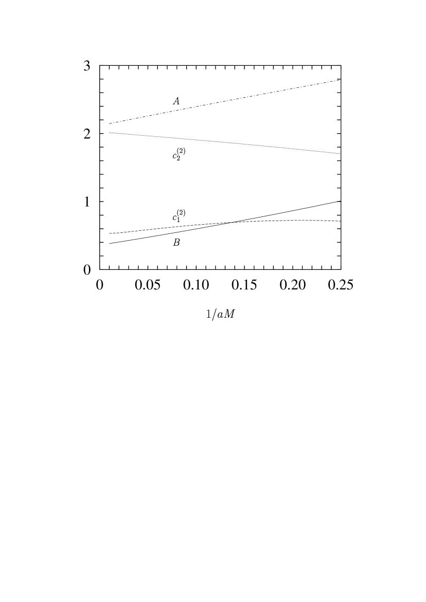
FIG. 3.: The energy shift parameter $A$, heavy-quark mass renormalization parameter $B$, and the kinetic coupling coefficients $c_{1}^{(2)}$ and $c_{2}^{(2)}$ before tadpole improvement ($u_{0}=1$) against $1/aM$ using $S_{G}^{(W)}$ and $\delta H^{(2)}$. The dot-dashed curve is $A$, the solid curve shows $B$, the dashed curve is $c_{1}^{(2)}$, and the dotted curve indicates $c_{2}^{(2)}$. The stability parameter $n$ is set to unity.

FIG. 4.: The shift $A$ in the zero point of energy, the heavy-quark mass renormalization parameter $B$, and the kinetic coupling coefficients $c_{1}^{(2)}$ and $c_{2}^{(2)}$ after tadpole improvement ($u_{0}=1-\alpha_{s}\pi/3$) against the product of the bare heavy-quark mass $M$ and the lattice spacing $a$ using $S_{G}^{(W)}$ and $\delta H^{(2)}$. The dot-dashed curve is $A$, the solid curve is $B$, the dashed curve is $c_{1}^{(2)}$, and the dotted curve indicates $c_{2}^{(2)}$. The stability parameter $n$ assumes the same values as used in Fig. 2.

FIG. 5.: The shift $A$ in the zero point of energy, the heavy-quark mass renormalization parameter $B$, and the kinetic coupling coefficients $c_{1}^{(2)}$ and $c_{2}^{(2)}$ after tadpole improvement ($u_{0}=1-\alpha_{s}\pi/3$) against $1/aM$ using $S_{G}^{(W)}$ and $\delta H^{(2)}$. The dot-dashed curve is $A$, the solid curve is $B$, the dashed curve is $c_{1}^{(2)}$, and the dotted curve indicates $c_{2}^{(2)}$. The stability parameter $n$ is set to unity.

FIG. 6.: The heavy-quark mass renormalization parameter $B$ against the product of the bare heavy-quark mass $M$ and the lattice spacing $a$. Results using the improved gluon action $S_{G}^{(I)}$ and the full set of NRQCD interactions $\delta H^{(4)}$ are shown as a solid curve. Results using $S_{G}^{(I)}$ and $\delta H^{(2)}$ are shown as a dot-dashed curve. The dashed curve indicates the results obtained using the simple gluon action $S_{G}^{(W)}$ with $\delta H^{(4)}$, while the dotted curve shows the results using $S_{G}^{(W)}$ with $\delta H^{(2)}$. The stability parameter $n$ assumes the same values as used in Fig. 2.

FIG. 7.: The heavy-quark wave function renormalization parameter $C$ against the product of the bare heavy-quark mass $M$ and the lattice spacing $a$ using $S_{G}^{(W)}$ and $\delta H^{(2)}$. The dashed curve shows $C$ before tadpole improvement $(u_{0}=1)$ and the solid curve shows $C$ after mean-field improvement $(u_{0}=1-\alpha_{s}\pi/3)$. The stability parameter $n$ assumes the same values as used in Fig. 2.

FIG. 8.: The energy shift scale $q^{\ast}_{A}$, heavy-quark mass renormalization scale $q^{\ast}_{B}$, and the kinetic coupling coefficient scales $q^{\ast}_{c_{1}^{(2)}}$ and $q^{\ast}_{c_{2}^{(2)}}$ before tadpole improvement ($u_{0}=1$) against the product of the bare heavy-quark mass $M$ and the lattice spacing $a$ using $S_{G}^{(W)}$ and $\delta H^{(2)}$. The dot-dashed curve is $aq^{\ast}_{A}$, the solid curve shows $aq^{\ast}_{B}$, the dashed curve is $aq^{\ast}_{c_{1}^{(2)}}$, and the dotted curve indicates $aq^{\ast}_{c_{2}^{(2)}}$. The stability parameter $n$ assumes the same values as used in Fig. 2.

FIG. 9.: The energy shift scale $q^{\ast}_{A}$, heavy-quark mass renormalization scale $q^{\ast}_{B}$, and the kinetic coupling coefficient scales $q^{\ast}_{c_{1}^{(2)}}$ and $q^{\ast}_{c_{2}^{(2)}}$ before tadpole improvement ($u_{0}=1$) against $1/aM$ using $S_{G}^{(W)}$ and $\delta H^{(2)}$. The dot-dashed curve is $aq^{\ast}_{A}$, the solid curve shows $aq^{\ast}_{B}$, the dashed curve is $aq^{\ast}_{c_{1}^{(2)}}$, and the dotted curve indicates $aq^{\ast}_{c_{2}^{(2)}}$. The stability parameter $n$ is unity.

FIG. 10.: The energy shift scale $q^{\ast}_{A}$, heavy-quark mass renormalization scale $q^{\ast}_{B}$, and the kinetic coupling coefficient scales $q^{\ast}_{c_{1}^{(2)}}$ and $q^{\ast}_{c_{2}^{(2)}}$ after tadpole improvement ($u_{0}=1-\alpha_{s}\pi/3$) against the product of the bare heavy-quark mass $M$ and the lattice spacing $a$ using $S_{G}^{(W)}$ and $\delta H^{(2)}$. The dot-dashed curve is $aq^{\ast}_{A}$, the solid curve shows $aq^{\ast}_{B}$, the dashed curve is $aq^{\ast}_{c_{1}^{(2)}}$, and the dotted curve indicates $aq^{\ast}_{c_{2}^{(2)}}$. The stability parameter $n$ assumes the same values as used in Fig. 2.

FIG. 11.: The energy shift scale $q^{\ast}_{A}$, heavy-quark mass renormalization scale $q^{\ast}_{B}$, and the kinetic coupling coefficient scales $q^{\ast}_{c_{1}^{(2)}}$ and $q^{\ast}_{c_{2}^{(2)}}$ after tadpole improvement ($u_{0}=1-\alpha_{s}\pi/3$) against $1/aM$ using $S_{G}^{(W)}$ and $\delta H^{(2)}$. The dot-dashed curve is $aq^{\ast}_{A}$, the solid curve shows $aq^{\ast}_{B}$, the dashed curve is $aq^{\ast}_{c_{1}^{(2)}}$, and the dotted curve indicates $aq^{\ast}_{c_{2}^{(2)}}$. The stability parameter $n$ is unity.

FIG. 12.: The first-order radiative corrections to the kinetic couplings $c_{1}$ and $c_{2}$ against $aM$ using $S_{G}^{(W)}$ and $\delta H^{(2)}$. The dashed curve is $\delta c_{1}=c_{1}^{(2)}\ \alpha_{V}(q^{\ast}_{c_{1}^{(2)}})$ and the dotted curve indicates $\delta c_{2}=c_{2}^{(2)}\ \alpha_{V}(q^{\ast}_{c_{2}^{(2)}})$, using $a\Lambda_{V}=0.169$. The stability parameter $n$ assumes the same values as used in Fig. 2.

FIG. 13.: Estimates of the energy shift $aE_{0}$ and mass renormalization $Z_{m}-1$ against $aM$ using $S_{G}^{(W)}$ and $\delta H^{(2)}$. The dot-dashed curves labeled $a$ and $b$ are energy shift estimates $A\ \bar{\alpha}_{V}(q^{\ast}_{A};\bar{q}_{A})$ for $\bar{q}_{A}=0.8/a$ and $0.6/a$, respectively, using $a\Lambda_{V}=0.169$ in $\alpha_{V}(\bar{q}_{A})$; the unlabeled dot-dashed curve is $A\ \alpha_{V}(q_{A}^{\ast})$. The solid curves labeled $c$ and $d$ show $B\ \bar{\alpha}_{V}(q^{\ast}_{B};\bar{q}_{B})$ for $\bar{q}_{B}=1.0/a$ and $0.6/a$, respectively; the unlabeled solid curve is $B\ \alpha_{V}(q^{\ast}_{B})$. Values for the stability parameter $n$ are the same as in Fig. 2.

REFERENCES

• [1] B.A. Thacker and G. Peter Lepage, Phys. Rev. D 43, 196 (1991).
• [2] G. Peter Lepage, Lorenzo Magnea, Charles Nakhleh, Ulrika Magnea, and Kent Hornbostel, Phys. Rev. D 46, 4052 (1992).
• [3] C. T. H. Davies and B. A. Thacker, Phys. Rev. D 45, 915 (1992).
• [4] Colin J. Morningstar, Phys. Rev. D 48, 2265 (1993).
• [5] C. Davies et al., “Precision $\Upsilon$ Spectroscopy from Nonrelativistic Lattice QCD,” in preparation.
• [6] C. Davies et al., “A New Determination of $M_{b}$ Using Lattice QCD,” SCRI-94-39, OHSTPY-HEP-T-94-004, submitted to Physical Review Letters.
• [7] This evolution equation differs slightly from that previously used in Refs. [2] and [4]. The NRQCD action was modified to simplify both perturbative and Monte Carlo computations.
• [8] G. Peter Lepage and Paul B. Mackenzie, Phys. Rev. D 48, 2250 (1993).
• [9] J. Mandula, G. Zweig, and J. Govaerts, Nucl. Phys. B228, 109 (1983).
• [10] Because the new NRQCD action is simpler than that studied previously, the procedure used here to evaluate the moments $\Omega_{m}^{(l)}$ differs slightly from that described in Ref. [4].
• [11] Results for both $\delta H^{(2)}$ and $\delta H^{(4)}$ using the simple Wilson $S_{G}^{(W)}$ and the $O(a^{2})$-improved $S_{G}^{(I)}$ gluonic actions are available in tabular form from the author.
Refer to caption