uprf-397-1994
Four loop result in Lattice Gauge Theory
by a Stochastic method:
Lattice correction to the condensate***
Research partially supported by murst, Italy.
F. Di Renzo, E. Onofri
Dipartimento di Fisica, Università di Parma and I.N.F.N., Gruppo
Coll. di Parma
G. Marchesini
Dipartimento di Fisica, Università di Milano and
I.N.F.N., Sezione di Milano
and
P. Marenzoni
Dipartimento di Scienze dell’Informazione, Facoltà di Ingegneria
Università di Parma, 43100 Parma (Italy)
May 1994
Abstract
We describe a stochastic technique which allows one to compute numerically the coefficients of the weak coupling perturbative expansion of any observable in Lattice Gauge Theory. The idea is to insert the exponential representation of the link variables into the Langevin algorithm and the observables and to perform the expansion in . The Langevin algorithm is converted into an infinite hierarchy of maps which can be exactly truncated at any order. We give the result for the simple plaquette of up to fourth loop order () which extends by one loop the previously known series.
1 Introduction
Weak coupling perturbation theory has been developed since the early times of Lattice Gauge Theory. While the lattice formulation provides the only method which allows for systematic non–perturbative calculations from first principles in strongly interacting asymptotically free theories, its perturbative expansion is also important. In particular weak coupling perturbation theory on the lattice is useful in order to accelerate the approach to the continuum, like in Symanzik’s improving program, or in the calculation of renormalization constants. For observables such as the gluon condensate or the topological susceptibility the weak coupling perturbative expansion on the lattice gives an important contribution to the Monte Carlo data (see Ref.[1, 2, 3, 4]). The expansion coefficients of the lattice correction to the gluon condensate and the topological susceptibility have been computed to three loop order [5] by means of a rather sophisticated diagrammatic technique.
We recently proposed [6] an alternative technique to compute numerically the coefficients of the expansion of any lattice observable based on Parisi–Wu [7] stochastic quantization implemented on the lattice [8]. The idea is simple: we insert the exponential map everywhere in the elementary Langevin evolution step. The stochastic evolution of the Lie–algebraic field depends parametrically on . We expand in powers of and obtain the evolution in the Langevin time order by order. By expanding the observable under consideration, the plaquette variable in the present study, it turns out that the coefficients of the perturbative expansion are given by expectation values of composite operators and are estimated as an average on the Langevin history.
A fundamental aspect of the approach is concerned with the problem of gauge fixing. We have found that the Langevin evolution with no gauge fixing is affected by a random fluctuation increasing in time and that this problem is taken care of by adopting a stochastic gauge fixing idea proposed by Zwanziger [9] and already implemented on the lattice [10].
In this paper we present an application of the method by computing the four loop coefficient of the plaquette expectation value which is related to the expectation value of the condensate . The first three coefficients agree with the known values.
We present the algorithm in some detail in section two. In section three we recall the stochastic gauge fixing method which is needed to keep statistical fluctuations finite. In section four we report the results obtained for the simple plaquette up to fourth loop order. In the final section we discuss the possibility of extracting the condensate from the plaquette Monte Carlo data and we comment on a possible scenario of high order perturbation theory.
2 The algorithm
We consider the standard pure gauge lattice action
| (1) |
where the sum extends to all plaquettes in a hypercubic lattice. We shall denote by the link variable at the site in the direction . We borrow the implementation of the Langevin dynamics from Ref.[8]. A single Langevin step is given by a sweep of the lattice where each link variable is updated according to the rule
| (2) |
where is given by
| (3) |
Here is the Langevin time step; the sum over means that gets contributions from all oriented plaquettes which include the link at ; the suffix traceless means that a subtraction of times the identity matrix is understood. Finally is extracted from a standard (antihermitian, traceless) Gaussian ensemble of –dimensional matrices. Now we represent by the exponential map on : . The Langevin evolution, when translated in terms of , is going to depend parametrically on . We then insert a formal power series expansion
| (4) |
into Eq. (2) and we try to match both sides order by order. To make this possible it is immediately evident that the time step must be scaled by putting , which is also expected since going to large requires smaller and smaller to avoid systematic errors. The Langevin algorithm has now been transformed into an infinite system of coupled non–linear stochastic finite–difference equations. The system can be truncated exactly at the desired order since each field is independent from higher order fields with ; in particular the field transforms by itself and represents the Abelian limit (a collection of gauge fields). The explicit form of the Langevin algorithm at any order can be obtained by expanding the products of link variables by Baker–Haussdorff–Campbell’s formula. Since our goal is to reach and, possibly, go beyond the order , we faced the problem of automatically generating these expansions. This was achieved using Mathematica††† Copyright © 1989-94 by Wolfram Research, Inc., which generates the algebraic expansion, optimizes the code trying to reduce the number of operations to a minimum and finally translates the output to (parallel) fortran or apese. Presently we are running the code designed to reach .
The explicit form of the expansion rapidly gets very cumbersome; to get a rough idea, the number of lines of text in the Mathematica output starts at 47 at order and it rises to 3544 at order . Hence we report the stochastic equations only for the first few orders (already specialized to )
| (5) | |||||
where we denote by the expansion coefficients of the unitary drift which are explicitly given to the first two orders by
| (6) |
Given the stochastic evolution order by order, we consider the expansion of any observable and we get
where is the value of the random variable, averaged over the whole lattice, after steps. The existence of the limit in terms of some “perturbative probability distribution” is still to be proven and it will be assumed as a working hypothesis here. This fact deserves further consideration in view of the fact that at first sight the behavior of the stochastic process is far from trivial.
3 Stochastic Gauge Fixing
The first run up to level was done without any gauge fixing. The evidence (see [6]) was rather strong in favour of the existence of the time average with an excellent agreement with the known values; however the statistical fluctuation of the signal at order 1 and 2 tends to increase in time signaling the fact that the asymptotic distribution, if it exists at all, has infinite second moments. The danger of such wild fluctuations in a numerical calculation is rather obvious – as soon as the signal/fluctuation ratio is smaller than the machine accuracy the algorithm is dead. While we are not able at present to suggest a precise picture of these fluctuations, it is believed that fixing the gauge is also going to fix the problem. Actually these large fluctuations can be thought of as gauge–non–invariant contributions to the time trajectory (with vanishing expectation) due to the fact that the full gauge invariance is only implemented by averaging on all possible noise–histories; for a given noise history stochastic time evolution and gauge transformations do not commute and this fact was considered responsible for this kind of fluctuations in Langevin dynamics (see [11]). The immediate source of divergence can be identified in the fields , which fluctuate like free Brownian variables in the absence of gauge–fixing. Higher order fields contain powers of and hence show stronger fluctuations. Fixing the gauge keeps the fields to bounded deviations and hence cures the problem. The kind of gauge fixing appropriate to Langevin dynamics was introduced by Zwanziger ([9]) and implemented as a lattice algorithm in [10]. The method consists in performing a gauge transformation after each sweep, in such a way that the field is attracted to the manifold defined by Landau gauge. The gauge transformation is given by
| (7) |
An iteration of by itself would bring the gauge potential to the Landau gauge. By interleaving it to each Langevin step one obtains a sort of soft gauge fixing, providing an additional drift which however does not modify the asymptotic probability distribution. We have now to expand the gauge fixing step in : this can be achieved with the same technique already developed for the unconstrained Lengevin algorithm. The parameter is chosen in order to minimize systematic errors — in practice it is set equal to .
4 Results
All the data will refer to the simple plaquette variable
| (8) |
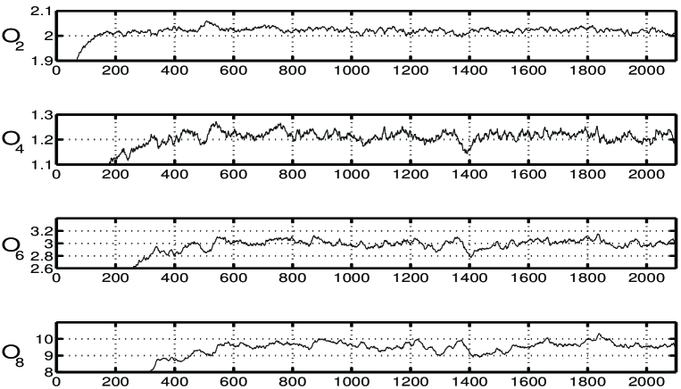
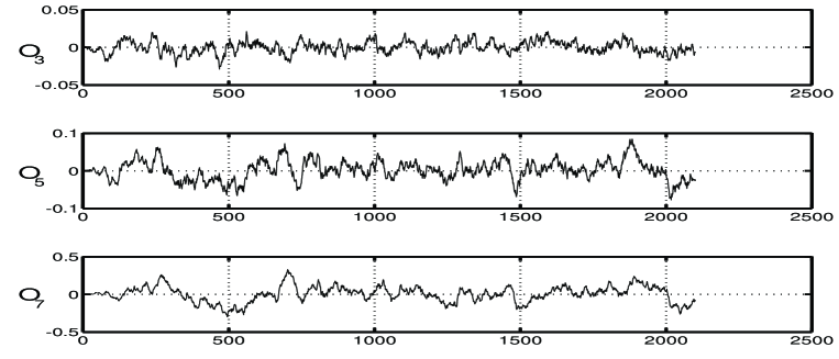
The expansion coefficients are obtained from the time average taken on a trajectory of 2100 Langevin steps of which the first 500 were discarded (see Fig. 1). The odd–degree operators , which must have vanishing expectation, are used to monitor the process (see Fig. 2).
The systematic error due to the finite evolution step can be corrected by running at different values of and extrapolating at (see Tab. 1). We check in this way that the method gives very accurate results when compared to the analytic results, but already for we need more statistics to get an improvement from the extrapolation in (see Fig. 3).
| 2.019 | 1.210 | 3.001 | 9.58 | |
| 0.001 | 0.002 | 0.014 | 0.09 | |
| 2.000(2) | 1.218(7) | - | - | |
| Exact | 2 | 1.212(7) | 3.12 | - |
Let us now discuss to what extent our calculation of the perturbative coefficients is different from those previously published. First of all, of course, there is an inherent statistical error, due to the stochastic nature of the calculation, which can be improved by accumulating more data.
Other sources of systematic errors, which are not seen with the present accuracy, may turn out to be relevant for other observables. First of all there are finite size effects: since we have to subtract the perturbative tail from Monte Carlo data taken on the same finite lattice, it could turn out that the right thing to do is not to correct for finite size at all. For a local quantity like the gluon condensate the finite size effect is going to be negligible anyway. Another difference from the standard calculation is more fundamental: we are not attempting to extract the leading term in the lattice spacing. Our result includes all irrelevant higher order terms in , which are also present in Monte Carlo data.
5 Discussion
Let us now recall from Ref. [1] that the single plaquette expectation obtained by Monte Carlo simulations on the lattice is related to the physical condensate by
| (9) |
where is the lattice perturbative correction discussed before. To two loop order the condensate in is given by the asymptotic freedom expression
| (10) |
where the constant is given by the physical quantity with the fundamental lattice gauge theory scale and where
are the first two perturbative coefficient of the -function.
The main question is then how to extract the physical condensate from the Monte Carlo data. First of all we perform the same analysis done in Ref. [1]: we try to estimate the gluon condensate by comparing with the various approximations given by
| (11) |
In Fig. 4 we report for by using the values of in Tab. 1 and the Monte Carlo results on the single plaquette reported in Ref. [4]. By increasing the perturbative order one sees that has a logarithmic slope in which decreases monotonically and seems to approach the asymptotic freedom slope in (10) given by the dotted line. The series seems still too short for . Following the same procedure as in Ref. [1], we introduce the next two coefficients and which we obtain by fitting with the asymptotic freedom expression in Eq. (10). Together with the two coefficients , one fits also the value of the condensate. The resulting points of are the lower points in Fig. 4 which are nicely fitted by the dotted line, the asymptotic freedom expression .
From the fit one obtains: , , and . This value of is close to the estimate obtained by performing the same analysis at one lower loop . Notice that, while the computed coefficients are all positive, the first unknown coefficient turns out to be negative. This is simply due to the fact that the functions have a slight curvature. Indeed, if one applies the same procedure at a lower loop, the first fitted coefficient turns out to be negative although the known value is positive.
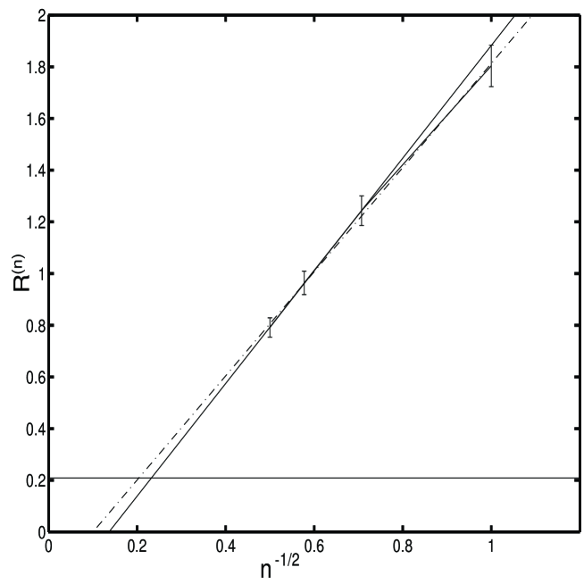
To analyze more closely the possible approach to asymptotic freedom, we plot in Fig. 5 the effective slopes of computed as follows. We perform a linear fit to in various intervals included in the interval where we expect to observe the asymptotic scaling. The result is shown in Fig. 5, by plotting vs. , the error bars being a measure of the different estimate of the slope depending on the interval chosen; the asymptotic freedom result is plotted as a horizontal line for comparison. It appears that the values of have a smooth behaviour as function of , which would however extrapolate to for a finite . This fact is typical of a divergent series. Indeed it has been observed [12, 13] that this should be the case due to the presence of renormalons. The leading renormalon gives the following large order behaviour of the expansion coefficients
| (12) |
As discussed in Ref. [13], this behaviour would imply that the intrinsic error in the estimate based on the divergent series would be of the same order of magnitude as the asymptotic freedom result . Actually for we find that the coefficients increase even faster with than the one in Eq. (12). This fact would make even more ambiguous the attempt to extract in this manner the gluon condensate from the Monte Carlo data. Thus one should find some new criterion to identify the perturbative subtraction. The stochastic calculation of should be available soon and we hope it will help in clarifying the situation.
We conclude by observing that our method can be easily adapted to evaluate high order perturbative expansions for any other gauge field observable, in particular we may correct for perturbative contributions to Wilson loops and to the topological susceptibility; the application to other models, such as chiral models on the lattice, should also be straightforward.
Acknowledgments
We thank warmly Prof. N. Cabibbo, A. Di Giacomo, A.H. Mueller, G. Parisi and Pietro Rossi for useful conversations. and Prof. G. Conte and the staff of the Computer Center of the Faculty of Engineering, University of Parma, for granting us computer time on their CM-2.
References
- [1] A. Di Giacomo and G.C. Rossi, Phys. Lett. 100B(6),(1981) 481–484.
- [2] T. Banks, R. Horsley, H.R. Rubinstein and U. Wolff, Nucl. Phys. B190 [FS3] (1981) 692–698.
- [3] G. Curci, G. Paffuti and R. Tripiccione, Nucl. Phys. B240[FS12] (1984) 91–112.
- [4] M. Campostrini, A. Di Giacomo and V. Gündük, Phys. Lett. 223 (1989) 393–397.
- [5] B. Allés, M. Campostrini, A. Feo and H. Panagopoulos, Nucl.Phys.(Proc.Suppl.) B34 (1994) and references therein.
- [6] F. DiRenzo, G. Marchesini, P. Marenzoni and E. Onofri, Nucl.Phys. (Proc.Suppl.) B34 (1994) 795.
- [7] G. Parisi and Wu Yongshi, Sci.Sinica Vol. XXIV N.4 (1981) 35.
- [8] G.G.Batrouni, G.R.Katz, A.S.Kronfeld, G.P.Lepage, B.Svetitsky and K.G.Wilson, Phys. Rev. D Vol. 32 No. 10 (1985) 2736.
- [9] D. Zwanziger, Nucl.Phys. B192 (1981) 259.
- [10] P.Rossi, C.T.H.Davies and G.P.Lepage, Nucl. Phys.B297 (1988) 287; C.T.H. Davies, G.G. Batrouni, G.R. Katz. A.S. Kronfeld, G.P. Lepage, K.G. Wilson, P. Rossi and B. Svetitsky, Phys. Rev. D 37 (1988) 1581–1588.
- [11] M. Falcioni, E. Marinari, M.L. Paciello, G. Parisi, B. Taglienti and Zhang Yi–Cheng, Nucl.Phys. B215 [FS7] (1983) 265–277; M. Falcioni, M.L. Paciello, G. Parisi and B. Taglienti, Nucl.Phys. B251 [FS13] (1985) 624–632.
- [12] G. Parisi, Phys.Lett. B76 (1977) 65; B. Lautrup, Phys. Lett. B69 (1978) 109; G. ’t Hooft, “Can we make sense out of Chromodynamics?”, “The Whys of subnuclear Physics”, Erice 1977, A. Zichichi Ed. (Plenum, New York, 1979) pag.943; G. Parisi, Nucl.Phys. B150 (1979) 163. F. David, Nucl.Phys. B234 (1984) 237; A.H. Mueller, Nucl.Phys. B250 (1985) 327.
- [13] V.I. Zakharov, Nucl.Phys. B385 (1992) 452–480.