April 1994 HLRZ 54/93         
BI-TP 93/76         
TIFR/TH/94-12         

Spatial and Temporal Hadron Correlators below and above
the Chiral Phase Transition
G. Boyd¹, Sourendu Gupta^1,3
F. Karsch^1,2 and E. Laermann²

¹ HLRZ, c/o Forschungszentrum Jülich, D-52425 Jülich, Germany

² Fak. f. Physik, Univ. Bielefeld, Postfach 100131, D-33501 Bielefeld, Germany

³ Present Address: TIFR, Homi Bhabha Road, Bombay 400005, India

Abstract

Hadronic correlation functions at finite temperature in QCD, with four flavours of dynamical quarks, have been analyzed both above and below the chiral symmetry restoration temperature. We have used both point and extended sources for spatial as well as temporal correlators. The effect of periodic temporal boundary conditions for the valence quarks on the spatial meson correlators has also been investigated. All our results are consistent with the existence of individual quarks at high temperatures. A measurement of the residual interaction between the quarks is presented.

1 Introduction

The spatial correlation functions of operators with hadronic quantum numbers yield screening masses for static excitations in the QCD plasma [1]. These give information on the physical excitations and interactions in QCD at finite temperatures. Chiral symmetry restoration at temperatures $T>T_{\mbox{\scriptsize c}}$ is signalled by the degeneracy of screening lengths obtained from pairs of opposite parity channels [1, 2, 3]. At such high temperatures, the vector (V), as well as the pseudovector (PV), screening mass is nearly twice the lowest Matsubara frequency, $\Omega=\pi T$, whereas the baryon screening mass is close to thrice this value. This indicates that correlations in these channels are mediated, respectively, by the exchange of two and three weakly interacting quarks [3].

Close to $T_{\mbox{\scriptsize c}}$, the scalar (S) and the pseudoscalar (PS) ‘meson’ screening mass is significantly smaller than the V/PV screening mass, but approaches the latter when the temperature is raised to $2T_{\mbox{\scriptsize c}}$ [4]. Thus, at high temperature, this channel is also correlated through the exchange of two weakly interacting quarks. Nevertheless, close to $T_{\mbox{\scriptsize c}}$, such an interpretation does not seem to hold.

Since the lowest mass hadron is unlikely to change from a mesonic collective state to a quark-like quasi-particle at a non-critical point, a pleasantly consistent picture of the excitation spectrum would be obtained if, above $T_{\mbox{\scriptsize c}}$, the S/PS correlations could be shown to be due to the propagation of two unbound quarks, possibly still strongly interacting close to $T_{\mbox{\scriptsize c}}$. A means of checking this was suggested and applied to quenched QCD [4]. This method also yielded measurements of effective couplings in different spin channels. It was seen that such a coupling is indeed larger in the S/PS channel than in the V/PV channel. In this paper we extend such studies to QCD with four flavours of dynamical staggered quarks.

Hadronic correlators, and similarly the spatial Wilson loops [5] and spatial four point functions with point-split sources [6], should provide information on the non-perturbative long distance structure of the quark gluon plasma. While the spatial and temporal quark propagators yield identical information about quark screening masses [7], this seems to be in conflict with recent studies of temporal and spatial hadron propagators [8]. In the latter case larger screening masses were extracted from temporal than from spatial correlators, although one would have expected to find smaller values as the lowest Matsubara mode is zero in this case. The determination of low momentum excitations from temporal propagators at finite temperature is, however, difficult, due to the short “time” extent of the lattice ($0<t<1/T$). This leads to a superposition of many high momentum excitations. We will try to clarify this situation here by projecting onto low momentum modes, by using wall source operators.

Furthermore, we will study the sensitivity of the extracted spatial screening lengths to changes of the temporal quark boundary conditions. While bosonic modes (bound states in mesonic operators) will not be sensitive to changes of the usual anti-periodic boundary conditions to periodic ones, fermionic modes (freely propagating quarks) will be sensitive to these changes. We will also extend the studies of scalar and vector channel couplings [4] to the case of QCD with dynamical fermions.

The conclusion from these investigations is that temporal and spatial propagators yield identical information on the spectrum of finite temperature QCD below and above the chiral phase transition. The behaviour of the (pseudo-)scalar screening length suggests that there are no bound states in this quantum number channel above $T_{\mbox{\scriptsize c}}$.

This paper is organized as follows. In section 2 we introduce the observables studied, and describe their behaviour for free staggered fermions, i.e., in the lowest order of perturbation theory. Details of our measurements and the results are given in section 3. A summary and conclusions are presented in the section 4.

2 Spatial and Thermal Direction Correlators

In this section we consider correlation functions between operators separated either in the spatial or the thermal direction. They are constructed on lattices of size $V=N_{\tau}\times N_{\sigma}^{3}$ with $N_{\sigma}>N_{\tau}$. Unless otherwise mentioned, we shall use the lattice spacing as the unit of length. The shorter direction introduces the temperature, via $N_{\tau}=1/T$. Spatial and thermal direction correlation functions with given external meson momentum $P_{\mu}$ are defined as

$$G_{s}^{H}(x_{3},\tilde{{\mbox{\boldmath$P$}}})\; = \;{1\over N_{\sigma}^{2}N_{\tau}}\sum_{\tilde{{\mbox{\boldmath$x$}}}}\langle H(x_{3},\tilde{{\mbox{\boldmath$x$}}})H^{\dagger}(0,\tilde{{\mbox{\boldmath$0$}}})\rangle\exp\left({i\tilde{{\mbox{\boldmath$P$}}}\cdot\tilde{{\mbox{\boldmath$x$}}}}\right),$$

$$G_{t}^{H}(x_{0},{\mbox{\boldmath$P$}})\; = \;{1\over N_{\sigma}^{3}}\sum_{{\mbox{\boldmath$x$}}}\langle H(x_{0},{\mbox{\boldmath$x$}})H^{\dagger}(0,{\mbox{\boldmath$0$}})\rangle\exp\left({i{\mbox{\boldmath$P$}}\cdot{\mbox{\boldmath$x$}}}\right).$$ (2.1)

For any 4-momentum $P_{\mu}$, we shall use the notation $\tilde{{\mbox{\boldmath$P$}}}$ to denote the 3-momentum $(P_{0},P_{1},P_{2})$, and $P$ for $(P_{1},P_{2},P_{3})$. Here $H$ denotes an operator carrying mesonic quantum numbers. By an abuse of language, we shall call $G_{s}$ and $G_{t}$ ‘meson correlators’. The name is not supposed to carry any prejudice about the existence or absence of mesons in the theory.

In perturbation theory, these correlation functions can be described in terms of the exchange of two (interacting) fermions. We set out our notation and introduce some features typical of non-interacting staggered fermions below. This corresponds to the leading order, ${\cal O}(g^{0})$, of perturbation theory. In section 3 the behaviour of the measured correlation functions will be compared with these features.

2.1 Spectral representations

Hadronic correlation functions at $T=0$ are used to extract the mass of the lowest excitation with given quantum numbers. A spectral representation of correlation functions with quantum numbers $H$, in the form

$$G^{H}(t)\;=\;\sum_{i}A_{i}{\rm e}^{-m_{H}^{i}t},$$ (2.2)

can be used to show that this necessitates the measurement of $G^{H}(t)$ at Euclidean time separations much larger than the splitting between the lowest and the first excited states, i.e., $t\gg 1/(m_{H}^{1}-m_{H}^{0})$. In the absence of any a priori knowledge of this splitting, it is necessary to take as large a time separation as possible, and to perform checks on the estimate of $m_{H}^{0}$ so obtained. All this is well known.

At finite temperatures the physical extent of the thermal direction, $\tau$, is bounded in physical units to $\tau\leq 1/T$. Due to the periodicity (or antiperiodicity) imposed to obtain the thermal ensemble, correlation functions can be followed only to $\tau\leq 1/(2T)$. In the general case this may not allow the extraction of the lowest lying state in the manner discussed above. One then has to use either a complicated ansatz for the correlation function, involving several exponentials to approximate eq. (2.2) [8], or a more complicated operator which projects out only the low momentum modes.

As the size of the spatial directions is not bounded in any way, it has become customary to study spatial rather than temporal correlation functions. The spatial correlation functions are the static correlations in the equilibrium system, and hence are also of direct physical relevance.

For the interpretation of the correlation functions measured in these simulations, one must discuss the spectral density functions underlying the correlations. While building models of the spectral densities, it is useful to keep certain constraints in mind. At finite temperatures the heat-bath provides a preferred frame of reference. As a result, the momentum representation of spectral functions is given in terms of $p_{0}$ and $|{\mbox{\boldmath$p$}}|$ separately, where ${\mbox{\boldmath$p$}}=(p_{1},p_{2},p_{3})$. Dynamical modes are defined by poles in the complex $p_{0}$ plane; and the movement of such poles with $|{\mbox{\boldmath$p$}}|$ are the dispersion relations. In examining the spectral representation of the thermal and spatial direction correlators it becomes clear that different aspects of the spectral function are important for each. However, information on the poles of spectral functions can be extracted from either of these correlators.

The residue at a pole can also be used to extract effective couplings. These are usually defined as the integrals of discontinuities over cuts in the complex plane of either $p_{0}$ or $|{\mbox{\boldmath$p$}}|$. Note that on any lattice the spectral function does not have any cuts, but only a set of poles. However, effective couplings can still be extracted via sums over the residues at the poles. One can expects finite lattice spacing effects to come from those poles which develop into a cut in the continuum limit.

2.2 Point Sources

In the staggered discretization, local operators for currents carrying mesonic quantum numbers are written in terms of fermion fields, $\chi(x)$, as

$$H(x)=\phi_{H}({\mbox{\boldmath$x$}})\overline{\chi}(x_{0},{\mbox{\boldmath$x$}})\chi(x_{0},{\mbox{\boldmath$x$}}).$$ (2.3)

The phase factors $\phi_{H}$ project onto definite quantum numbers [9], and are listed in Table 1, for the channels analyzed in this study.

Table 1: Phases for the meson operators used for $G_{t}^{H}$. For $G_{s}^{H}$, $x_{3}$ should be replaced by $x_{0}$. Also listed are kinematic factors appearing in the ${\cal O}(g^{0})$ perturbative calculations of the meson correlation functions in eqs. (2.4) and (2.6).

Channel	$\phi_{H}({\mbox{\boldmath$x$}})$	$f^{H}_{\mbox{\scriptsize even}}$	$f^{H}_{\mbox{\scriptsize odd}}$
S	$1$	$m^{2}-\omega\omega^{\prime}$	1
PS	$(-1)^{x_{1}+x_{2}+x_{3}}$	$m^{2}+\omega\omega^{\prime}$	1
PV	$(-1)^{x_{1}}+(-1)^{x_{2}}+(-1)^{x_{3}}$	$3m^{2}-\omega\omega^{\prime}$	3
V	$(-1)^{x_{1}+x_{2}}+(-1)^{x_{2}+x_{3}}+(-1)^{x_{1}+x_{3}}$	$3m^{2}+\omega\omega^{\prime}$	3

Since the meson operators, $H(x)$, are composed of fermion operators, it is clear that even for a fixed external meson momentum, $\tilde{{\mbox{\boldmath$P$}}}$ or $P$, quarks with a spectrum of internal momenta will contribute to the correlation functions $G_{s}^{H}$ and $G_{t}^{H}$. The structure of the hadronic correlation functions is, therefore, more complicated than that of the quark correlator [7].

This is clear when the correlation functions at ${\cal O}(g^{0})$ are explicitly written out. For the spatial correlation function the result is well known:

$$G_{s}^{H}(x_{3},\tilde{{\mbox{\boldmath$P$}}})/T^{3}\;=\;\frac{24N_{\tau}^{3}}{N_{\tau}N_{\sigma}^{2}}\sum_{\tilde{{\mbox{\boldmath$p$}}}}f^{H}G^{q}_{s}(x_{3},\tilde{{\mbox{\boldmath$p$}}})G^{q}_{s}(x_{3},\tilde{{\mbox{\boldmath$p$}}}^{\prime}).$$ (2.4)

The factors $f^{H}$ for even and odd sites are given in Table 1. The quark propagator $G^{q}_{s}$ is given by:

$$G_{s}^{q}(x_{3},\tilde{{\mbox{\boldmath$p$}}})\;=\;\left\{\begin{array}[]{lr}{\displaystyle\frac{\sinh[E_{s}(x_{3}-N_{\sigma}/2)]}{\sinh(E_{s}N_{\sigma}/2)\cosh E_{s}}}&(x_{3}{\mbox{ odd}})\\ {\displaystyle\rule{0.0pt}{25.83325pt}\frac{\cosh[E_{s}(x_{3}-N_{\sigma}/2)]}{\sinh(E_{s}N_{\sigma}/2)\sinh 2E_{s}}}&(x_{3}{\mbox{ even}})\\ \end{array}\right.$$ (2.5)

The temporal correlation function is very similar:

$$G_{t}^{H}(x_{0},{\mbox{\boldmath$P$}})/T^{3}\;=\;\frac{24N_{\tau}^{3}}{N_{\sigma}^{3}}\sum_{{\mbox{\boldmath$p$}}}f^{H}G_{t}^{q}(x_{0},{\mbox{\boldmath$p$}})G_{t}^{q}(x_{0},{\mbox{\boldmath$p$}}^{\prime}),$$ (2.6)

with the quark propagator $G_{t}^{q}$ given by

$$G_{t}^{q}(x_{0},{\mbox{\boldmath$p$}})\;=\;\left\{\begin{array}[]{lr}{\displaystyle\frac{\cosh[E_{t}(x_{0}-N_{\tau}/2)]}{\cosh(E_{t}N_{\tau}/2)\cosh E_{t}}}&(x_{0}{\mbox{ odd}})\\ {\displaystyle\rule{0.0pt}{25.83325pt}\frac{\textstyle\sinh[E_{t}(x_{0}-N_{\tau}/2)]}{\textstyle\cosh(E_{t}N_{\tau}/2)\sinh 2E_{t}}}&(x_{0}{\mbox{ even}})\\ \end{array}\right.$$ (2.7)

The sums in eqns. (2.4) and (2.6) are over internal quark momenta. These run over $p_{0}=(2n+1)\pi T$ and $p_{i}=2n\pi T$, with $i=1$, 2, 3 and $n=0,\pm 1,\cdots$ . The quark and antiquark momenta, $p$ and $p^{\prime}$ respectively, sum to give the meson momentum $P$, i.e. $P_{\mu}=p_{\mu}+p^{\prime}_{\mu}$. We have used the abbreviation

$$E_{t,s}\;=\;\mbox{arcsinh}(\omega_{t,s}),$$ (2.8)

along with the definitions

$$\omega_{t}^{2}=m_{\mbox{\scriptsize q}}^{2}+\sum_{k=1}^{3}\sin^{2}(p_{k})\qquad{\mbox{ and}}\qquad\omega_{s}^{2}=m_{\mbox{\scriptsize q}}^{2}+\sum_{k=0}^{2}\sin^{2}(p_{k}).$$ (2.9)

The variables $E^{\prime}$ and $\omega^{\prime}$ are obtained by replacing $p$ by $p^{\prime}$, and $m_{\mbox{\scriptsize q}}$ is the bare quark mass.

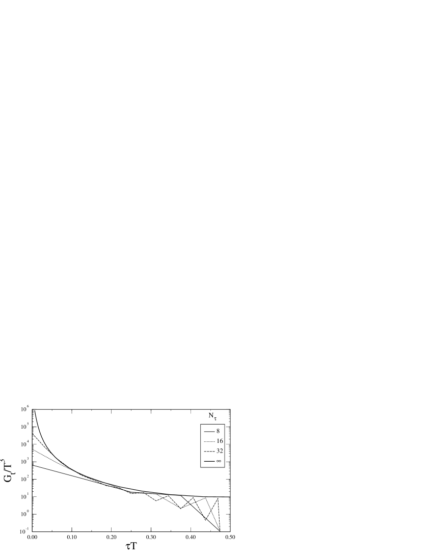
Figure 1: Thermal direction correlation functions at ${\cal O}(g^{0})$ on lattices with $N_{\sigma}\to\infty$ and various $N_{\tau}$ values. The quark mass is $m_{\mbox{\scriptsize q}}=0.01$, and we define $\tau T=x_{0}/N_{\tau}$. The result for $N_{\tau}\to\infty$ is obtained from eq. (2.11).

Recall that the spectrum of $p_{0}$ starts from the Matsubara frequency, $\Omega=\pi T$, and reflects the antiperiodic boundary conditions usually imposed in the thermal direction on the fermion fields when inverting the Dirac equation. All other momentum components start from zero. As a result, the screening mass at $O(g^{0})$ is independent of the meson operator $H$ and given by [3]

$$\mu_{H}\;=\;2E_{\mbox{\scriptsize s}}^{\mbox{\tiny min}}\;=\;2\mbox{arcsinh}\left({m_{\mbox{\scriptsize q}}^{2}+\sin^{2}\Omega}\right).$$ (2.10)

The decay of $G_{s}^{H}$ at $x_{3}\gg 1/T$ is controlled by $\mu_{H}$. At shorter distances the higher modes also contribute and lead to a more rapid decrease of the correlation function. At very short distances, $x_{3}<1/(2T)$, all terms in the sums in eq. (2.4) turn out to be important.

The thermal direction correlation function, $G_{t}^{H}$, does not yield extra information in perturbation theory. Since $x_{0}<1/(2T)$, all terms in the sum in eq. (2.6) turn out to be important, and the correlation function falls very rapidly due to the contribution of terms with large $E_{t}$ and $E^{\prime}_{t}$. This is shown in Figure 1. Also shown in the same figure is the result obtained letting first $N_{\sigma}$ and then $N_{\tau}\to\infty$ at fixed $T$. The formulæ in eqs. (2.6) and (2.7) then reduce to the continuum expressions for the correlators constructed from non-interacting quarks. For zero external momentum, ${\mbox{\boldmath$P$}}=0$, and vanishing quark masses, these take on the simple form

$$G_{t}^{H}(\tau,{\mbox{\boldmath$P$}}=0)\;=\;{96T^{3}\over\pi^{2}}\int_{0}^{\infty}dy{y^{2}\over\cosh^{2}y}\cosh^{2}\bigl{(}y(2T\tau-1)\bigr{)}$$ (2.11)

where $y$, $\tau$ and $T$ are related to the lattice variables via $\tau=x_{0}a$, $\tau T=x_{0}/N_{\tau}$ and $y=E_{t}/(2T)$. Notice that, at short distances, one obtains $G_{t}^{H}(\tau,{\mbox{\boldmath$P$}}=0)\sim\tau^{-3}$ from eq. (2.11). (Similar conclusions have been reached in the continuum, [10].)

Although the temporal direction is too short to single out the lowest excitation for $T>0$, it is still instructive to study the behaviour of local masses, $m(x_{0})$, obtained from $G_{t}^{H}$. These are obtained by comparing the correlation functions on successive even (or odd) lattice sites, $x_{0}\pm 1$. One then solves

$${G_{t}^{H}(x_{0}-1,{\mbox{\boldmath$0$}})\over G_{t}^{H}(x_{0}+1,{\mbox{\boldmath$0$}})}\;=\;{\cosh\left[m(x_{0})(x_{0}-1-N_{\tau}/2)\right]\over\cosh\left[m(x_{0})(x_{0}+1-N_{\tau}/2)\right]}\,,$$ (2.12)

for $m(x_{0})$. The left hand side is obtained from either a measured or perturbatively calculated correlation function. One then assumes on the right hand side that the correlation function can be described by an ordinary meson correlator consisting of a single cosh. (For the simple case of non-interacting quarks we know, of course, that we should rather use the sum over squares of quark correlators applicable to the given source and sink.) A feeling for this local mass may be obtained by noting that in the limit $N_{\tau}\to\infty$, at fixed $T$ (i.e., $a\to 0$), eq. (2.11) can be used to show that

$$m(x_{0})x_{0}=m(\tau)\tau\;\simeq\;3\qquad(N_{\tau}\gg x_{0}\gg 0).$$ (2.13)

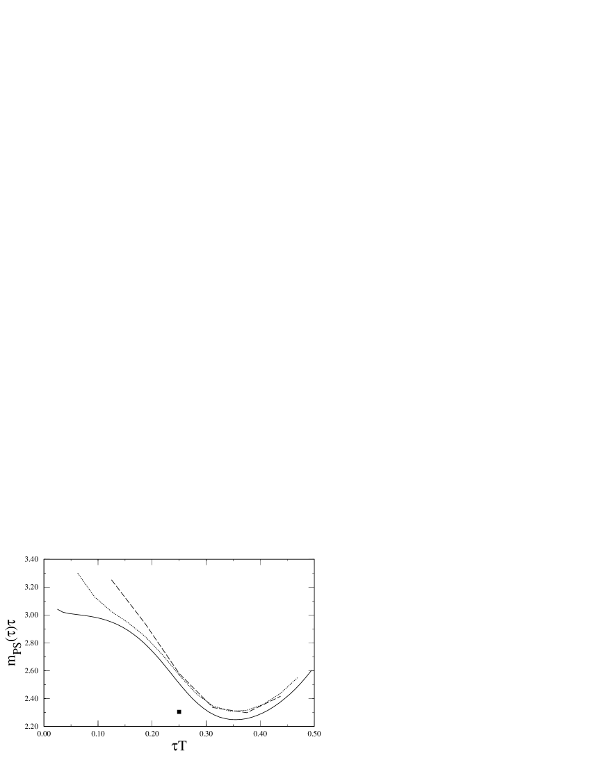
Figure 2: Scaled local masses at $O(g^{0})$, $m(\tau)\tau$, versus the scaled separation $\tau T=x_{0}/N_{\tau}$, obtained from eqs. (2.6) and (2.7) for $N_{\sigma}\to\infty$ for $N_{\tau}=16$ (dashed line) and 32 (dotted line). The full line shows the result for $N_{\tau}=\infty$ (eq. (2.11)). The filled square shows the result for $m(\tau=0.25/T)$ on an $8\times 16^{3}$ lattice.

Analytic results for the local masses at ${\cal O}(g^{0})$ in perturbation theory are shown in Figure 2. Note that, in practice, $m(\tau)\tau$ remains close to 3 for all values of $\tau T$. The rise of the local meson mass at short distances, when extracted in this fashion, reflects the increasing importance of higher momentum excitations. We note that even for the largest possible separation $x_{0}=N_{\tau}/2$, or equivalently $\tau=1/(2T)$, the local mass remains large in units of the temperature, $m/T\approx 6$. The result for $\tau=1/(4T)$, obtained on an $8\times 16^{3}$ lattice, is also shown in the figure. This is the only value of $\tau$ which we will be able to study numerically.

As a concluding remark to this section, let us point out a distinctive feature of a meson propagator consisting of non-interacting quarks, $G_{t}^{H}(x_{0})$, namely the strong oscillation between even and odd sites visible in Figure 1. This is seen for any non-zero lattice spacing (finite $N_{\tau}$), and persists in higher orders of perturbation theory. Such oscillatory behaviour is also seen in the spatial correlation functions in perturbation theory. In the low-temperature phase of QCD, however, where one has a genuine bound state, the correlator does not show such a behaviour.

2.3 Wall Sources

From the previous discussion we conclude that the analysis of the correlation functions (and especially the temporal correlation functions) between local hadronic operators is complicated, owing to the momentum sums in eqs. (2.4) and (2.6). A determination of the low momentum excitations through local masses or fits with a few exponentials seems to be difficult, as all higher energy levels, coming from higher quark momenta, contribute.

The contributions from higher quark momenta can be suppressed by the judicious choice of a wall source, which creates quarks with only the lowest allowed momentum. For correlations measured in the thermal direction, the boundary conditions on the transverse slice are periodic. In this case one can project onto zero quark momentum via the meson sources

$$H_{\mbox{\scriptsize wall}}(x_{0},{\mbox{\boldmath$x$}})={8\over N_{\sigma}^{3}}\sum_{\stackrel{{\scriptstyle{\mbox{\boldmath$e$}},{\mbox{\boldmath$e^{\prime}$}}}}{{\mbox{\scriptsize even}}}}\phi_{H}({\mbox{\boldmath$x$}})\overline{\chi}(x_{0},{\mbox{\boldmath$x$}}+{\mbox{\boldmath$e$}})\chi(x_{0},{\mbox{\boldmath$x$}}+{\mbox{\boldmath$e$}}^{\prime}).$$ (2.14)

For correlators measured in the spatial direction, the antiperiodic boundary condition in the thermal direction means that one can not project onto zero momentum. Instead a projection onto the Matsubara momentum $\tilde{{\mbox{\boldmath$\Omega$}}}=(\pi T,0,0)$ must be used:

$$H_{\Omega}(x_{3})={8\over N_{\sigma}^{2}N_{\tau}}\sum_{\stackrel{{\scriptstyle{\mbox{\boldmath$e$}},{\mbox{\boldmath$e^{\prime}$}}}}{{\mbox{\scriptsize even}}}}\phi_{H}(\tilde{{\mbox{\boldmath$x$}}})\overline{\chi}(x_{3},\tilde{{\mbox{\boldmath$x$}}}+\tilde{{\mbox{\boldmath$e$}}})\chi(x_{3},\tilde{{\mbox{\boldmath$x$}}}+\tilde{{\mbox{\boldmath$e$}}}^{\prime})\exp\left({i(\tilde{{\mbox{\boldmath$e$}}}-\tilde{{\mbox{\boldmath$e$}}}^{\prime})\cdot\tilde{{\mbox{\boldmath$\Omega$}}}}\right).$$ (2.15)

The correlation functions are measured between a wall source and a point sink, with a sum over all sinks in the plane transverse to the direction of propagation.

The $O(g^{0})$ perturbative calculation in eqs. (2.4) and (2.6) is simplified if the only contribution is from quarks with momentum ${\mbox{\boldmath$p$}}={\mbox{\boldmath$0$}}$ or $\tilde{{\mbox{\boldmath$p$}}}=\tilde{{\mbox{\boldmath$\Omega$}}}$. For example, the temporal correlator becomes the square of a single quark propagator,

$$G_{t}^{H,\mbox{\scriptsize wall}}(x_{0},{\mbox{\boldmath$0$}})/T^{3}\;=\;3(N_{\tau}^{3}/N_{\sigma}^{3})f^{H}G_{t}^{q}(x_{0},{\mbox{\boldmath$0$}})G_{t}^{q}(x_{0},{\mbox{\boldmath$0$}}).$$ (2.16)

The biggest gain in using extended sources is obtained for the thermal direction correlation functions. At ${\cal O}(g^{0})$ in perturbation theory the masses are then given by

$$m^{\mbox{\scriptsize wall}}\;=\;2\mbox{arcsinh}\left(m_{\mbox{\scriptsize q}}\right).$$ (2.17)

Local masses can then be extracted by using eq. (2.12). We note that at ${\cal O}(g^{0})$ the meson correlator now has the form $\cosh^{2}(m_{\mbox{\scriptsize q}}(x_{0}-N_{\tau}/2))$, which is well fitted by a $\cosh(2m_{\mbox{\scriptsize q}}(x_{0}-N_{\tau}/2))$ over most of the temporal range.

At ${\cal O}(g^{0})$ in perturbation theory the local masses thus measure the mass of the lowest excitation. At higher orders this is modified due to diagrams which can be separated into thermal corrections to each of the quark propagators and interactions between the propagating quark and antiquark. Each of these effects begins at ${\cal O}(gT)$. If the effective interaction between the two quarks can be neglected, as we expect for the V channel, then the effect of interactions can be wholly subsumed into replacing the quark mass $m_{\mbox{\scriptsize q}}$ in eq. (2.17) by the thermal quark mass, $m_{\mbox{\scriptsize q}}^{\mbox{\scriptsize eff}}$. This was extracted from the temporal quark correlator in [7] using the same configurations used here. It is not unrealistic to hope that such a result may hold beyond perturbation theory as well.

2.4 Varying Boundary Conditions

In our attempt to clarify the nature of the excitations in the plasma we have also varied the temporal boundary condition on the valence fermion fields from which the meson operators are constructed. The boundary conditions of the sea quarks, driving the generation of the gauge field ensemble, have been left untouched. This should give a direct view of the nature of excitations in the plasma.

If the lowest excitation in a channel of fixed quantum numbers consists of a meson, then the spectral representation contains a pole. Thus, we are assured that this state will be seen in the correlation of generic operators with these quantum numbers. In particular, whether we use periodic or anti-periodic boundary conditions on the fermion source, the lowest mass obtained out of the correlation functions must be the same. The correlation functions should thus show little dependence on the choice of boundary conditions.

However, if a given quantum number can only be obtained by exchanging more than one particle, then the spectral representation contains a cut. If the exchanged particles are fermions, then the contribution to the correlation function depends on the boundary conditions. In fact, at ${\cal O}(g^{0})$, it is easy to see that eqs. (2.4) and (2.5), which define the spatial correlation functions, depend on the temporal boundary conditions via the spectrum of $p_{0}$ alone. For periodic boundary conditions in the thermal direction, the allowed values are $p_{0}=2n\pi T$ with $n=\{0,1,\cdots\}$, which yields a screening mass equal to

$$\mu\;=\;2E_{s}^{\mbox{\scriptsize min}}\;=\;2\mbox{arcsinh}(m_{\mbox{\scriptsize q}}).$$ (2.18)

The qualitative change in going from anti-periodic to periodic boundary conditions in the thermal direction is thus expected to be significant, and should show up in the correlation functions. Interactions will modify this in the same way as discussed above.

2.5 Effective inter-quark Couplings

One may use the meson propagators to calculate an effective four fermion coupling as used in, for example, the Nambu–Jona-Lasinio model [11]. The propagator at zero four-momentum is equal to the generalised susceptibility [4],

$$\chi_{\pi,\rho}=\tilde{G}_{\pi,\rho}(0).$$ (2.19)

Letting $\tilde{G}_{\pi,\rho}^{0}(0)=\chi_{\pi,\rho}^{0}$ be the susceptibility for non-interacting quarks in the pion and rho channels respectively, one obtains from the Dyson equation the result:

$$\chi_{\pi,\rho}=\frac{\chi_{\pi,\rho}^{0}}{1-g_{\pi,\rho}\chi_{\pi,\rho}^{0}},$$ (2.20)

where $g_{\pi,\rho}/2$ is the four fermion coupling in the effective Lagrangian, following the convention of [11].

Solving for $g_{\pi,\rho}$ one obtains:

$$g_{\pi,\rho}T^{2}=\frac{1}{N_{\tau}^{2}}\left(\frac{1}{\chi_{\pi,\rho}^{0}}-\frac{1}{\chi_{\pi,\rho}}\right),$$ (2.21)

where the susceptibility extrapolated to zero quark mass is used.

3 Results

In this section we describe the results of our measurements on configurations generated by the $MT_{\mbox{\scriptsize c}}$ collaboration on lattices of size $8\times 16^{3}$ with 4 flavours of dynamical fermions having a bare mass $m_{\mbox{\scriptsize q}}a=0.01$. Recall that the phase transition was observed at a coupling of $\beta=5.15(5)$ [12]. At this coupling we have two sets of configurations. The set labelled B corresponds to a run which started in the low-temperature (chiral symmetry broken) phase and remained there. The set labelled S was started in the high-temperature (chirally symmetric) phase and did not tunnel into the other phase. The couplings $\beta=5.1$ and $5.2$ cover the temperature range $T/T_{\mbox{\scriptsize c}}=1\pm 0.2.$

Results are presented for both point sources and wall sources. For the wall sources we have fixed the configurations to the Coulomb gauge in the hyperplane containing the source, transverse to the direction of propagation.

We have around twenty configurations at each value of the coupling, with four sources per configuration for point sources, and one for wall sources. In calculating the errors for the point sources we first blocked the four sources. The errors quoted reflect the statistical fluctuations alone.

3.1 Thermal direction point source correlators

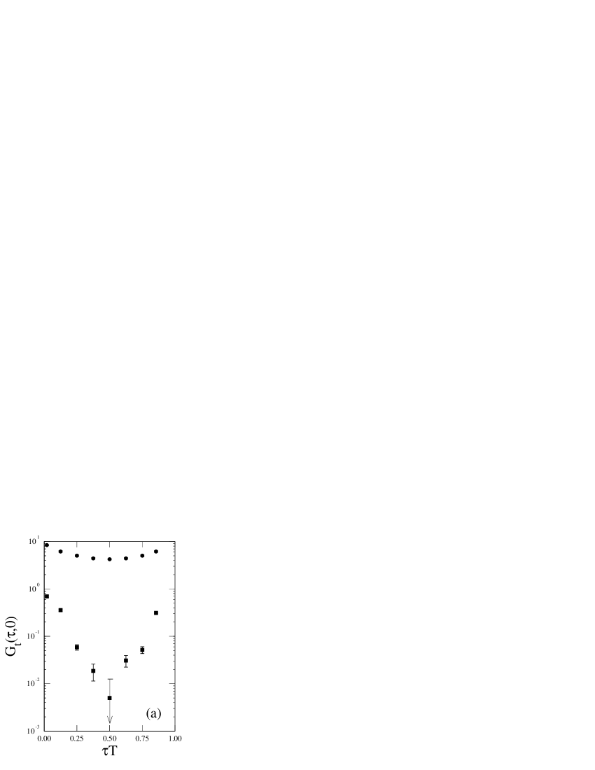
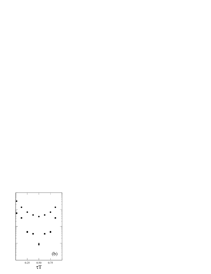
Figure 3: The thermal direction correlators for PS (filled circles) and V (filled squares) at $\beta=5.1$ (a), 5.3 (b) and 6.5 (c), shown as a function of $\tau T$. In (c) the lowest order results for PS (solid line) and V (dashed line) correlators are also shown.

The measured values of $G_{t}^{H}$ are shown in Figure 3. Note that the pseudoscalar correlator for $T<T_{\mbox{\scriptsize c}}$ is very well described by a hyperbolic cosine. A changeover to the oscillatory behaviour characteristic of free fermions, as discussed in the previous section, is visible in our thermal correlation functions as the critical coupling, $\beta_{\mbox{\scriptsize c}}=5.15$, is crossed. This change in behaviour is most noticeable when wall sources are used. Note also that the oscillation between even and odd sites is enhanced in the vector channel. This is in accordance with the perturbative calculation, and is due to the fact that $f^{V}\geq f^{PS}$ (see Table 1).

In Figure 5 we show the local masses at distance $\tau=0.25/T$ extracted from the V and PS correlation functions using eq. (2.12), (and hence the implied ansatz,) in the thermal direction. These are also listed in Table 2. We find that the local mass in the V channel is close to the perturbative value, $m_{V}=9.4/T$ (see Figure 2). However, the local mass in the PS channel approaches this value rather slowly with increasing temperature. Such a behaviour is very similar to that of the screening masses extracted from spatial correlation functions.

Table 2: Local masses from thermal direction V and PS correlation functions at distance $\tau=1/(4T)$. Results obtained from point and wall source operators are shown. For comparison we also list twice the effective quark mass [7].

$\rule{0.0pt}{12.91663pt}\beta$	$m_{PS}^{\mbox{\scriptsize point}}$	$m_{V}^{\mbox{\scriptsize point}}$	$m_{PS}^{\mbox{\scriptsize wall}}$	$m_{V}^{\mbox{\scriptsize wall}}$	$2m_{\mbox{\scriptsize q}}^{\mbox{\scriptsize eff}}$
5.1	0.24(5)	1.5(2)			0.9(1)
5.15(B)	0.36(7)	1.2(1)			0.6(1)
5.15(S)	0.46(6)	1.19(9)	0.29(1)	0.56(1)	0.42(6)
5.2	0.51(6)	1.08(8)	0.31(1)	0.493(5)	0.38(4)
5.3	0.64(4)	1.13(6)	0.303(6)	0.401(5)	0.19(9)
6.5	0.98(2)	1.13(3)	0.0838(4)	0.106(2)	0.044(8)

These local masses are similar in magnitude to the screening masses. This is accidental. It is due to the fact that for $N_{\tau}=8,N_{\sigma}=16$ we can only extract a local temporal mass at $\tau T=1/4$. In a free fermion theory on this size lattice we find that the local mass at this distance is about $10T$. This just happens to be close to the meson screening mass in free fermion theory on this size lattice, $9T$. When the lattice size is changed, this accidental concordance is removed (see eq. (2.13)).

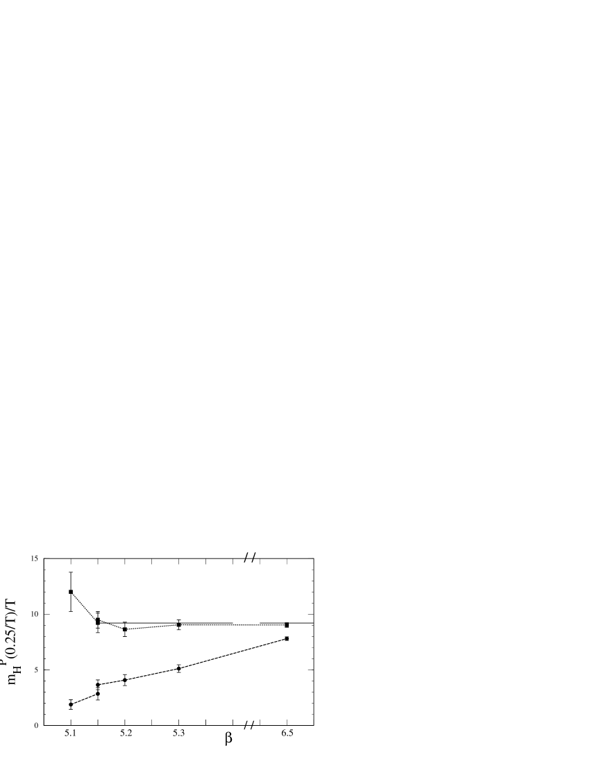
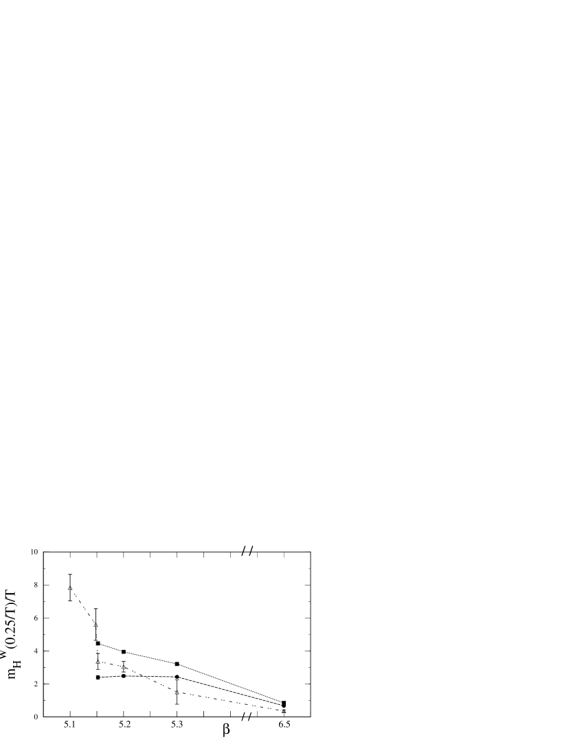
Figure 4: Local masses $m_{\mbox{\scriptsize H}}^{\mbox{\scriptsize P (=point)}}$ at distance $\tau T=1/4$ from thermal direction V (squares) and PS (circles) correlation functions using point sources, shown as a function of $\beta$. Also shown is the corresponding result computed in a theory of non-interacting fermions on an $8\times 16^{3}$ lattice at the same $\tau$ (full line).

Figure 5: Local masses $m_{\mbox{\scriptsize H}}^{\mbox{\scriptsize W (=wall)}}$ from correlators constructed with wall sources in the PS (circles) and V (squares) channels in the high temperature phase. Also shown is $2m_{q}^{\mbox{\scriptsize eff}}$ (triangles) from [7]. Lines have been drawn to guide the eye.

3.2 Thermal direction wall source correlators

Local masses have similarly been extracted from the temporal wall source correlators. The results obtained for $m^{\mbox{\scriptsize wall}}$ are also collected in Table 2. We note that these masses are indeed much smaller than the local masses obtained using point sources. The projection onto the lowest momentum excitation with these correlation functions thus seems to be rather efficient.

The relation in eq. (2.17) seems to hold, at least qualitatively, for both the vector and the pseudo-scalar channels, when the effective quark mass $m_{\mbox{\scriptsize q}}^{\mbox{\scriptsize eff}}$ given in [7] is used for the quark mass. The masses in the PS channel close to $\beta_{\mbox{\scriptsize c}}$ are smaller than those in the vector channel, indicating strong residual interactions between fermions. The PS masses then approach the mass in the vector channel as the coupling increases.

We also note that the vector mass remains larger than $2m_{\mbox{\scriptsize q}}^{\mbox{\scriptsize eff}}$, indicating the importance of the remaining inter-quark interactions. One may try to parametrize these residual interactions in a potential model relating the difference in the pion and rho masses to different spin–spin interactions in these quantum number channels. The masses then receive contributions from the effective quark masses, as well as the scalar ($E_{\mbox{\scriptsize scalar}}$) and spin dependent ($E_{\mbox{\scriptsize spin}}$) part of the quark–anti-quark potential:

$$m_{PS} = 2m_{\mbox{\scriptsize q}}^{\mbox{\scriptsize eff}}+E_{\mbox{\scriptsize scalar}}-\frac{3}{4}E_{\mbox{\scriptsize spin}}$$ (3.1)

$$m_{V} = 2m_{\mbox{\scriptsize q}}^{\mbox{\scriptsize eff}}+E_{\mbox{\scriptsize scalar}}+\frac{1}{4}E_{\mbox{\scriptsize spin}}.$$ (3.2)

We find that the meson masses can then be parametrized by a scalar term that is consistent with zero, and a spin term approximately equal to the effective quark mass, and with the same temperature dependence.

3.3 Anti-Periodic and Periodic Boundary Conditions

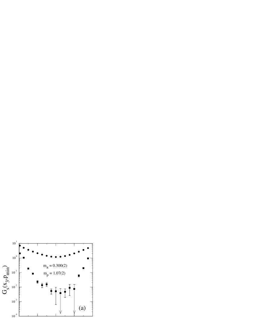
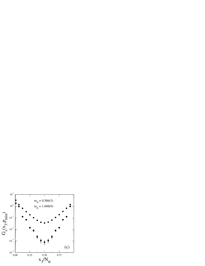
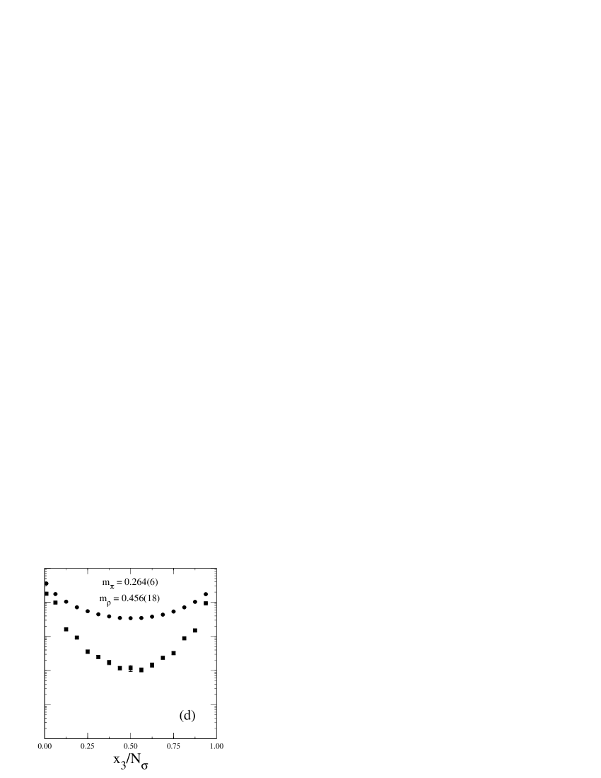
Figure 6: $G_{s}^{H}$ in the PS (circles) and V (squares) channels. Figures (a) and (b) correspond to $\beta=5.1$, while figures (c) and (d) correspond to $\beta=5.3$. The valence quarks have anti-periodic boundary conditions in the thermal direction for (a) and (c), with (b) and (d) having periodic boundary conditions in the thermal direction. The masses shown were obtained from fits.

In Figure 6 (a) and (b) $G_{s}^{PS}$ and $G_{s}^{V}$ are shown for $T<T_{\mbox{\scriptsize c}}$ for both periodic (per) (a) and anti-periodic (aper) (b) boundary conditions in the thermal direction. The correlation functions are unaffected by this change, and the screening masses, shown in Table 3, do not change within errors. Thus, these masses reflect bosonic poles in the spectral function.

In contrast, there is a remarkable difference between the correlation functions obtained for periodic and anti-periodic boundary conditions for $T>T_{\mbox{\scriptsize c}}$, as shown in Figure 6 (c) and (d). The correlation functions become much flatter when the boundary conditions are periodic, and the screening mass drops in both the PS and V channels. Varying the boundary conditions thus suggests the absence of genuine mesons in the high temperature phase of QCD.

It can be seen that the vector screening mass $\mu_{V}^{\mbox{\scriptsize per}}$ closely satisfies the relation in eq. (2.18), when the quark mass is taken to be the non-perturbative quark mass measured at the same coupling [7]. Thus, the effects of interactions, in this angular momentum channel, can be almost entirely lumped into the effective quark mass. (This relation also holds below the transition, and gives a definition of the constituent quark mass.) As is already known [4], this simplification does not hold in the $PS$ channel, and an effective interaction between quarks remains. The value of $\mu_{PS}^{\mbox{\scriptsize per}}$ is accordingly somewhat smaller than $\mu_{V}^{\mbox{\scriptsize per}}$.

Table 3: Screening masses in the PS and V channels for both anti-periodic (aper) and periodic (per) boundary conditions in the thermal direction. In the chirally symmetric phase results obtained with wall source operators (W) are also quoted. The screening mass expected for this size lattice, using non-interacting quarks, is $2\pi T=1.2$ for point sources and $2\pi T=1.0$ for wall sources.

$\rule{0.0pt}{12.91663pt}\beta$	$\mu_{PS}^{\mbox{\scriptsize aper}}$	$\mu_{PS}^{\mbox{\scriptsize per}}$	$\mu_{V}^{\mbox{\scriptsize aper}}$	$\mu_{V}^{\mbox{\scriptsize per}}$
5.1	0.300(2)	0.296(4)	1.07(2)	1.07(1)
5.15(B)	0.296(7)	0.301(5)	1.15(1)	0.84(5)
5.15(S)	0.394(6)	0.299(7)	0.947(7)	0.68(3)
5.15(SW)		0.270(3)		0.552(3)
5.2	0.469(7)	0.294(8)	0.979(10)	0.548(18)
5.2(W)		0.259(3)		0.463(3)
5.3	0.578(5)	0.264(6)	1.048(9)	0.456(18)
5.3(W)	0.553(4)	0.218(5)	0.820(2)	0.337(6)
6.5	0.899(3)	0.112(9)	1.101(3)	0.113(21)

In Table 3 and Figure 7 results for screening masses from the wall source operators (eq. (2.15)) are presented. These are a little smaller than those obtained from point source operators, which indicates that the spatial direction is not large enough to eliminate higher terms in the sum in eq. (2.4). Presumably, slightly larger spatial lattices would be required for this. Experience from [4] shows that spatial sizes $N_{\sigma}\approx 4N_{\tau}$ generally suffice to eliminate the effect of the higher modes.

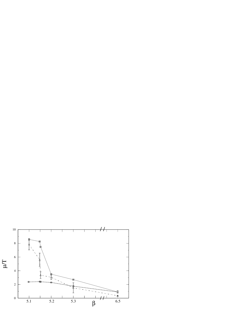
Figure 7: Screening masses extracted from spatial correlation functions using point sources with periodic temporal boundary conditions. Shown is the rho (squares) and pion (circles) screening mass, extracted in both cases from fits to the correlator on even sites. Also shown is twice the effective quark mass (triangles) determined on the same gauge field configurations in the Landau gauge [7]. Lines are drawn to guide the eye.

The values of $\mu_{H}^{\mbox{\scriptsize per}}$ are similar to the values of local masses extracted from wall source operators in the thermal direction. This is indeed to be expected in perturbation theory. At ${\cal O}(g^{0})$ these two masses should be the same, while differences can arise at higher orders in $g$. Thus in the limit $m_{\mbox{\scriptsize q}}\to 0$, both these quantities are sensitive to $O(gT)$ thermal corrections. The screening masses in Figure 7 may be compared with the wall source results shown in Figure 5.

3.4 Effective inter-quark Couplings

The effective four fermion coupling, defined in eq. (2.21), is presented in table 4. Notice that the coupling in the pion channel is about four times stronger than that in the rho channel, supporting the hypothesis that the difference between the pion and rho screening masses lies in different interaction strengths between the quarks in the two channels. The numbers obtained at the transition are also comparable with those obtained in the quenched approximation [4].

Table 4: Effective four fermion couplings for the pion $(g_{\pi})$ and rho $(g_{\rho})$ in the limit of zero quark mass. The susceptibilities for non-interacting quarks are: $1/\chi^{0}_{\pi}=0.5478$ and $1/\chi^{0}_{\rho}=0.3680$.

$\rule{0.0pt}{12.91663pt}\beta$	$g_{\pi}T^{2}$	$g_{\rho}T^{2}$
5.15(S)	0.00795(6)	0.00184(10)
5.2	0.00785(8)	0.00189(11)
5.3	0.0074(1)	0.00184(15)
6.5	0.005(8)	0.0010(4)

Taking the transition temperature to be $T_{c}=0.14$GeV [13] the following physical values for the couplings in the chirally symmetric phase at the transition are obtained: $g_{\pi}=0.41$GeV^-2 and $g_{\rho}=0.094$GeV^-2. These numbers may be compared with the values quoted in [11], obtained from fits to the experimental meson data at $T=0$: $g_{\pi}=4.90$GeV^-2 and $g_{\rho}=3.25$GeV^-2. The couplings at high temperature are well below the critical coupling at which the Nambu–Jona-Lasinio model first shows chiral symmetry breaking, and provide a further indication that neither channel has a low lying bound state.

4 Conclusions

The pion and rho correlators are, above the phase transition, sensitive to both the boundary conditions and the type of source used. This is not seen below the phase transition. Since the changes in the correlator are of the form one expects if unbound fermions play a direct role in the spectral function, this provides evidence for the existence of a two fermion cut dominating the spectral function.

Above the phase transition the screening masses in both the PS and vector channels are consistent with twice the effective quark mass plus some residual interactions. As a measure of this interaction, and hence as a summary of the relevant physics of the system, we extracted an effective four fermion coupling. This was four times stronger for the PS channel than it was for the vector channel, and an order of magnitude smaller than the couplings used in Nambu–Jona-Lasinio models at zero temperature.

The structure of correlators in the vector channel above $T_{\mbox{\scriptsize c}}$ generally agrees quite well with the behaviour expected from leading order perturbation theory; however, this is not the case for the pseudo-vector channel below $2T_{\mbox{\scriptsize c}}$. Here the correlators and masses are seen to approach the perturbation limit rather slowly.

One is left with a consistent picture of a plasma phase consisting of deconfined, but strongly interacting quarks and gluons in the temperature range from $T_{\mbox{\scriptsize c}}$ to $2T_{\mbox{\scriptsize c}}$.

References

- [1] C. DeTar and J. Kogut, Phys. Rev. Lett., 59 (1987) 399; Phys. Rev., D36 (1987) 2828.
-
[2]
S. Gottlieb, W. Liu, R. L. Renken, R. L. Sugar, and D. Touissant,
Phys. Rev. Lett., 59 (1987) 1881;
A. Gocksch, P. Rossi and U. M. Heller, Phys. Lett., B205 (1988) 334. - [3] K. Born, S. Gupta, A. Irbäck, F. Karsch, E. Laermann, B. Petersson and H. Satz, Phys. Rev. Lett., 67 (1991) 302.
- [4] S. Gupta, Phys. Lett., B288 (1992) 171.
-
[5]
C. Borgs, Nucl. Phys., B261 (1985) 455;
E. Manousakis and J. Polonyi, Phys. Rev. Lett., 58 (1987) 847. - [6] C. Bernard, M.C. Ogilvie, T. DeGrand, C. DeTar, S. Gottlieb, A. Krasnitz, R. Sugar and D. Toussaint, Phys. Rev. Lett., 68 (1992) 2125.
- [7] G. Boyd, S. Gupta and F. Karsch, Nucl. Phys., B385 (1992) 481.
- [8] T. Hashimoto, T. Nakamura and I. O. Stamatescu, Nucl. Phys.B400 (1993) 267.
- [9] M. Golterman, Nucl. Phys., B273 (1986) 663.
- [10] W. Florkowski and B. L. Friman, Z. Phys. A 347 (1994) 271.
- [11] S. Klimt, M. Lutz, U. Vogl, and W. Weise Nucl. Phys., A516 (1990) 429
- [12] R. V. Gavai, S. Gupta, A. Irbäck, F. Karsch, S. Meyer, B. Petersson, H. Satz and H. W. Wyld, Phys. Lett., B241 (1990) 567.
- [13] R. Altmeyer, K. D. Born, M. Göckeler, R. Horsley, E. Laermann and G. Schierholz, Nucl. Phys., B389 (1993) 445.