Hadron Masses from the Valence Approximation

to Lattice QCD

F. Butler, H. Chen, J. Sexton, A. Vaccarino,

and D. Weingarten

IBM Research

P.O. Box 218, Yorktown Heights, NY 10598

ABSTRACT

We evaluate pseudoscalar, vector, spin 1/2 and spin 3/2 baryon masses predicted by lattice QCD with Wilson quarks in the valence (quenched) approximation for a range of different values of lattice spacing, lattice volume and quark mass. Extrapolating these results to physical quark mass, then to zero lattice spacing and infinite volume we obtain values for eight mass ratios. We also determine the zero lattice spacing, infinite volume limit of an alternate set of five quantities found without extrapolation in quark mass. Both sets of predictions differ from the corresponding observed values by amounts consistent with the predicted quantities’ statistical uncertainties.

1 INTRODUCTION

In a recent letter [1] we summarized a lattice QCD calculation of the masses of eight low-lying hadrons, extrapolated to physical quark mass, zero lattice spacing, and infinite volume, using Wilson quarks in the valence (quenched) approximation. This approximation may be viewed as replacing the momentum and frequency dependent color dielectric constant arising from quark-antiquark vacuum polarization with its zero momentum, zero frequency limit and might be expected to be fairly reliable for low-lying baryon and meson masses [2]. In the present article we describe the hadron mass calculation of Ref. [1] in greater detail.

Each of the eight predicted mass ratios which we obtain is within 6% of experiment. The difference between the predicted ratios and experiment is less than 1.6 times the corresponding statistical uncertainty. It appears to us reasonable to take these results as quantitative confirmation of the mass predictions both of QCD and of the valence approximation. We believe it is unlikely that the valence approximation would agree with experiment for eight different mass ratios yet differ significantly from QCD’s predictions including the full effect of quark-antiquark vacuum polarization.

For the four lattices used in our extrapolations to physical mass ratios, we calculate hadron masses for a range of quark masses above $0.3m_{s}$, where $m_{s}$ is the strange quark mass. We do not calculate hadron masses directly at smaller quark mass because below $0.3m_{s}$ our algorithms become unacceptably slow. For quark masses ranging from about $0.3m_{s}$ to $1.1m_{s}$ we find pseudoscalar meson masses squared, vector meson masses, and baryon masses to be very close to linear functions of the quark mass. The masses of nonstrange hadrons are then found by extrapolating these linear fits down to $m_{n}$, the average of the up and down quark masses. Recent calculations based on chiral perturbation theory [3, 4] show that at sufficiently small quark mass a peculiarity of the valence approximation might lead to significant deviations from our linear extrapolations. In Ref. [5] evidence is discussed which suggests that this potential difficulty occurs mainly at very small quark mass and probably does not have an effect on our extrapolations from $0.3m_{s}$ down to $m_{n}$. In the present article we will also show that hadron masses in the real world are quite close to linear functions of valence quark masses over the range of our extrapolations. The linearity of observed hadron masses as functions of valence quark masses is closely related to the success of the Gell-Mann-Okubo mass formula.

An alternate interpretation of our mass calculations can be made, however, which does not depend on extrapolation in quark mass. The linearity of real world hadron masses as a function of quark mass implies that all masses in each hadron multiplet are determined by the first two coefficients of a Taylor series expansion around any quark mass between $m_{n}$ and $m_{s}$. Our data shows that for the valence approximation this linearity occurs at least between $0.3m_{s}$ and $1.1m_{s}$. Our results can then be cast as predictions of the first two Taylor coefficients for each hadron multiplet at some conveniently chosen quark mass between $0.3m_{s}$ and $1.1m_{s}$. Four of our five predicted values for these coefficients at the point $(m_{n}+m_{s})/2$ differ from experiment by less than 1.6 times the corresponding statistically uncertainty. The fifth prediction differs by 2.0 times its statistical uncertainty. The predicted constant terms are within 6.5% of experiment with statistical uncertainties of up to 3.3%. The predicted coefficients of the linear terms in these expansions lie within 22% of experiment with statistical uncertainties of up to 22%. The coefficients of the linear terms are obtained from small differences between the masses of hadrons with different quark compositions and as a result have relatively large statistical errors.

Following Refs. [6, 7], we also determine the coupling constant $g^{(0)}_{\overline{MS}}$ from the lattice coupling constant $g_{lat}$. From $g^{(0)}_{\overline{MS}}$, by the two-loop Callan-Symanzik equation, we determine $\Lambda^{(0)}_{\overline{MS}}a$ in units of lattice spacing $a$. The values we find for the ratio $(\Lambda^{(0)}_{\overline{MS}}a)/(m_{\rho}a)$ are constant within statistical errors. Thus $m_{\rho}a$ depends on $a$ according to asymptotic scaling to within statistical errors. This result tends to support the reliability of our extrapolation of masses to the continuum limit. The infinite volume, continuum limit of $\Lambda^{(0)}_{\overline{MS}}/m_{\rho}$ combined with the value of $m_{\rho}$ in physical units permits a calculation of $\Lambda^{(0)}_{\overline{MS}}$ in physical units. The result we obtain agrees, to within 4% statistical errors, with a value of the infinite volume, continuum limit $\Lambda^{(0)}_{\overline{MS}}$ obtained from a charmonium mass splitting [6].

An evaluation of meson decay constants using the data set from which masses are extracted here is discussed in detail in Ref. [8].

The calculations described here were done on the GF11 parallel computer at IBM Research [9] and took approximately one year to complete. The machine was used in configurations ranging from 384 to 480 processors, with sustained speeds ranging from 5 Gflops to 7 Gflops. With the present set of improved algorithms and 480 processors, these calculations could be repeated in about four months.

2 COULOMB GAUGE HADRON OPERATORS

For all but one choice of lattice size and $\beta$, we construct hadron propagators with nonlocal source and sink operators. The operators which we use are specified in lattice Coulomb gauge. A transformation to lattice Coulomb gauge is defined to give a local maximum of the sum over all sites and space direction links

$$\sum_{x,i=1,2,3}ReTr[U_{i}(x)].$$ (2.1)

A transformation which produces a local maximum of this sum is found by a method qualitatively similar to the Cabbibo-Marinari-Okawa Monte Carlo algorithm. The lattice is swept repeatedly, and at each site the target function is maximized first by a gauge transformation in the $SU(2)$ subgroup of $SU(3)$ acting only on gauge index values 1 and 2, then by a gauge transformation in the $SU(2)$ subgroup acting only on index values 2 and 3, then by a gauge transformation in the subgroup acting only on index values 1 and 3. Maximizing the target function over $SU(2)$ subgroups is easier to program than a direct maximization over all of $SU(3)$. On the other hand, it is not clear that maximizing each site over $SU(3)$ would significantly accelerate the full transformation to Coulomb gauge. A local maximum is reached when at each site the quantity $R(x)$ vanishes where

$$Q(x) = \sum_{i}[U_{i}(x)-U_{i}^{\dagger}(x-\hat{i})],$$

$$R(x) = Q(x)-Q^{\dagger}(x)-\frac{2}{3}ImTr[Q(x)].$$ (2.2)

The vector $\hat{i}$ is a unit lattice vector in the positive $i$ direction. We stop the iteration process when the sum over the lattice of the quantity $Tr[R^{\dagger}(x)R(x)]$ becames smaller than a convergence parameter $c$.

In Coulomb gauge, a smeared quark field $\phi_{r}(\vec{x},t)$ is then constructed from the local quark field $\psi(\vec{x},t)$ by

$$\phi_{r}(\vec{x},t) = \sum_{\vec{y}}G_{r}(\vec{x}-\vec{y})\psi(\vec{y},t),$$

$$G_{r}(\vec{z}) = (\sqrt{\pi}r)^{-3}exp(-\frac{|\vec{z}|^{2}}{r^{2}}).$$ (2.3)

Spin, flavor and color indices have been suppressed in Eq. (2). The field $\overline{\phi}_{r}(\vec{x},t)$ is defined by a corresponding smearing of $\overline{\psi}(\vec{x},t)$. We take the smeared fields $\phi_{0}(x)$ and $\overline{\phi}_{0}(x)$ to be $\psi(x)$ and $\overline{\psi}(x)$, respectively.

Smeared hadron fields can then be formed from local products of smeared quark and antiquark fields. The fields for a charged pion and a changed rho are

$$\pi^{+}_{r}(x) = \overline{\phi}^{d}_{r}(x)\gamma^{5}\phi^{u}_{r}(x)$$

$$\rho^{+i}_{r}(x) = \overline{\phi}^{d}_{r}(x)\gamma^{i}\phi^{u}_{r}(x).$$ (2.4)

For a proton, antiproton, $\Delta^{++}$ or $\overline{\Delta^{++}}$ with with z-component of spin given by $s$ we have the nonrelativistic operators

$$P^{s}_{r}(x) = \phi^{u}_{air}(x)\phi^{u}_{bjr}(x)\phi^{d}_{ckr}(x)\epsilon_{abc}\Gamma^{Ps}_{ijk}$$

$$\overline{P}^{s}_{r}(x) = \overline{\phi}^{u}_{air}(x)\overline{\phi}^{u}_{bjr}(x)\overline{\phi}^{d}_{ckr}(x)\epsilon_{abc}\Gamma^{\overline{P}s}_{ijk}$$

$$\Delta^{s}_{r}(x) = \phi^{u}_{air}(x)\phi^{u}_{bjr}(x)\phi^{u}_{ckr}(x)\epsilon_{abc}\Gamma^{\Delta s}_{ijk}$$ (2.5)

$$\overline{\Delta}^{s}_{r}(x) = \overline{\phi}^{u}_{air}(x)\overline{\phi}^{u}_{bjr}(x)\overline{\phi}^{u}_{ckr}(x)\epsilon_{abc}\Gamma^{\overline{\Delta}s}_{ijk}$$

where $a$, $b$ and $c$ are color indices, $i$, $j$, and $k$ are spinor indices, $\epsilon_{abc}$ is the alternating index, and repeated indices are summed over. For gamma matrices which are the same as the Bjorken and Drell convention, but with space direction matrices multiplied by $i$, the nonzero components of the baryon spin wave functions with maximum spin in the z-direction are

$$\Gamma^{P1/2}_{112} = -\Gamma^{P1/2}_{121}=1,$$

$$\Gamma^{\overline{P}1/2}_{443} = -\Gamma^{\overline{P}1/2}_{434}=1,$$

$$\Gamma^{\Delta 3/2}_{111} = 1,$$ (2.6)

$$\Gamma^{\overline{\Delta}3/2}_{444} = 1.$$

Corresponding smeared fields can be defined for other nucleon and delta charge and spin sates, and for other pseudoscalar mesons, vector mesons, and spin 1/2 and 3/2 baryons.

Hadron field operators obtained from local products of gaussian smeared fields, when fourier transformed, are equivalent to operators formed from local fields with nonlocal gaussian relative wave functions. For a pion at rest, for example, we have

$$\sum_{\vec{x}}\pi^{+}_{r}(\vec{x},t)=\sum_{\vec{y}\vec{z}}G_{s}(\vec{z})\overline{\psi}^{u}(\vec{y},t)\gamma^{5}\psi^{d}(\vec{y}+\vec{z},t),$$ (2.7)

where $s$ is $\sqrt{2}r$.

From Coulomb gauge smeared fields for each hadron we constructed zero momentum, spin summed hadron propagators for a collection of source and sink sizes. For a hadron $h$, the propagator is

$$c^{h}_{rr^{\prime}}(t) = \sum_{\vec{x}s}<[h^{s}_{r}(\vec{x},t)]^{\dagger}h^{s}_{r^{\prime}}(0,0)>$$ (2.8)

The invariance of lattice QCD under parity and charge conjugation transformations gives a variety of equalities among various pairs of propagators. Propagators which should be equal can be added together to decrease statistical fluctuations. For a lattice with time direction period $T$, our final zero-momentum propagators are then

$$C^{\pi}_{rr^{\prime}}(t) = c^{\pi}_{rr^{\prime}}(t)+c^{\pi}_{rr^{\prime}}(T-t),$$

$$C^{\rho}_{rr^{\prime}}(t) = c^{\rho}_{rr^{\prime}}(t)+c^{\rho}_{rr^{\prime}}(T-t),$$

$$C^{P}_{rr^{\prime}}(t) = c^{P}_{rr^{\prime}}(t)+c^{\overline{P}}_{rr^{\prime}}(t),$$ (2.9)

$$C^{\Delta}_{rr^{\prime}}(t) = c^{\Delta}_{rr^{\prime}}(t)+c^{\overline{\Delta}}_{rr^{\prime}}(t),$$

with corresponding definitions for other mesons and baryons.

For a lattice with a sufficiently large space direction periodicity $S$, statistical fluctuations in hadron propagators can, in principle, be further decreased by introducing several gaussian sources, each multiplied by a random cube root of 1 to cancel cross terms between the propagation of different sources for both baryon and meson propagators. A closely related idea was first proposed in Ref. [10]. If $S$ is large and even, for example, a quark field with eight sources is

$$\phi^{\prime}_{r}(t)=\sum_{\vec{y}}\xi_{\vec{y}}\phi_{r}(\vec{y},t),$$ (2.10)

for $\phi_{r}$ of Eq. (2). Each component of the eight $\vec{y}$ included in the sum in Eq. (2.10) is either 0 or $S/2$, and the $\xi_{\vec{y}}$ for each different $\vec{y}$ and each different gauge configuration used to find quark propagators are independent random cube roots of 1. Using $\phi^{\prime}_{r}$ of Eq. (2.10) to define hadron source operators but with $\phi_{r}$ of Eq. (2) still used to define sink operators, a new set of hadron propagators $C^{\prime h}_{rr^{\prime}}(t)$, $h=\pi,\rho,P,\Delta$, can be constructed similar to those in Eq. (2). If $S$ is sufficiently large, however, the $C^{\prime h}_{rr^{\prime}}(t)$ found from any ensemble of gauge fields will behave as though they have been averaged over eight times as many independent gauge configurations as corresponding $C^{h}_{rr^{\prime}}(t)$

3 PROPAGATORS

Table 1 lists the lattice sizes and parameter values for which quark and hadron propagators were evaluated. Up and down quark masses were taken to be equal in all propagators. We therefore obtained degenerate masses for each isospin multiplet of hadrons. This approximation leads to almost no loss in useful results since since the observed values of mass splittings in isospin multiplets in the real world are generally somewhat smaller than our statistical errors. We also did no calculations directly including strange quarks. Masses for hadrons including strange quarks were found by an extrapolation in quark mass to be discussed in Section 6. Direct calculations including strange quarks would have required additional programming but would have increased our required computer time by only a small fraction.

We chose periodic boundary conditions in all directions for both gauge fields and quark fields. Gauge configurations were generated using a version of the Cabbibo-Marinari-Okawa [11] algorithm adapted for parallel computers by Ding [12]. The number of sweeps skipped between configurations and the total count of configurations for each set of lattice parameters are given in the last two columns of the table. Values of the correlation between hadron propagators on successive pairs of gauge configurations we found to be statistically consistent with zero. Thus the number of sweeps between configurations in each case was sufficient to produce statistically independent hadron propagators on all gauge configurations used in the calculation of propagators.

For the $8^{3}\times 32$ lattice at $\beta$ of 5.7, we used point sources and sinks in the quark propagators. For all other lattices we used gaussian sources with $r$ of 2, and four different gaussian sinks, with $r$ of 0, 1, 2 and 3. For all lattices except $24^{3}\times 32$ at $\beta$ of 5.7, we found propagators for the source fields of Eq. (2) including a single source. For $24^{3}\times 32$ at $\beta$ of 5.7 we found propagators for the source fields of Eq. (2.10) including eight sources.

For all the lattices listed in Table 1, the gauge transformation convergence parameter $c$ defined following Eq. (2) was set to $10^{-5}$. The average number of sweeps required for convergence to this accuracy ranged from 1525 on the lattice $24^{3}\times 36$ at $\beta$ of 5.93, to 2270 on the lattice $16^{3}\times 32$ at $\beta$ of 5.7.

Quark propagators were constructed using the conjugate gradient algorithm for the $8^{3}\times 32$ lattice at $\beta$ of 5.7, using red-black preconditioned conjugate gradient for the other lattices at $\beta$ of 5.7 and 5.93, and using a red-black preconditioned minimum residual algorithm at $\beta$ of 6.17 [13]. At the largest hopping constant values at $\beta$ of 5.7 and 5.93, preconditioning the conjugate gradient algorithm increased its speed by a factor of 3, and at the largest hopping constant values at $\beta$ of 6.17, the change from conjugate gradient to the minimum residual algorithm yielded an additional factor of 2 in speed. Table 2 gives the average number of lattice sweeps needed to find quark propagators for all of the lattice sizes and parameter values which we use to find infinite volume continuum limit masses. The number of sweeps in all cases was chosen large enough to insure that effective pion, rho, nucleon and delta masses evaluated within the time interval used for final fits are within 0.2% of their values obtained on propagators run to machine precision. The number of sweeps required to obtain this precision was found by calculating propagators with several different convergence criteria on small ensembles of configurations.

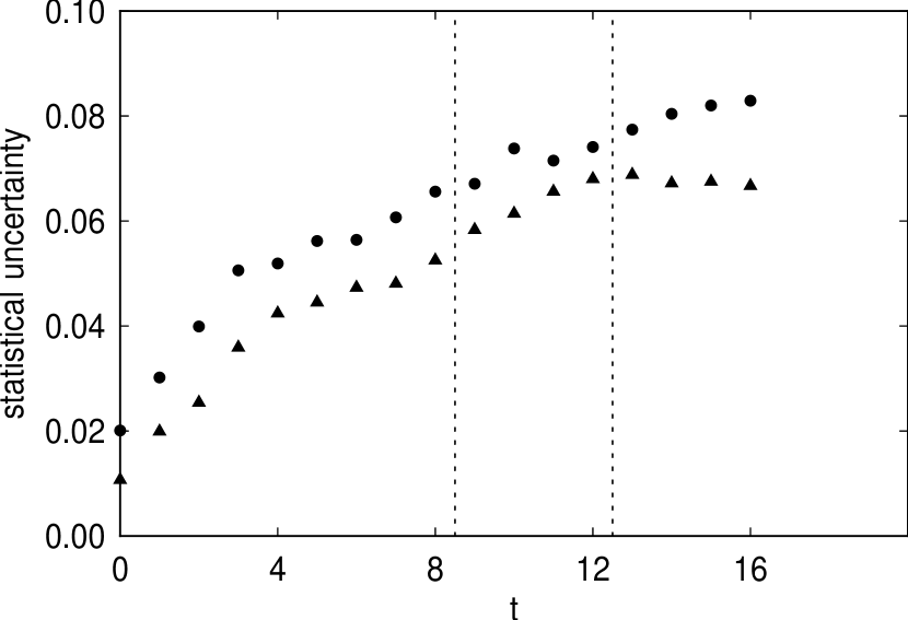
Figure 6: Fractional uncertainty in the pion propagator obtained from one source (circles) and from eight sources (triangles) on the lattice $24^{3}\times 32$ at $\beta=5.70$ and $k=0.1675$.

At $\beta$ of 5.7 we also found propagators for the lattice $16^{3}\times 32$ using a source field including eight sources for an ensemble of 81 configurations. For the lattice $24^{3}\times 32$ additional propagators were found using a source field including only a single source for an ensemble of 18 configurations. Figures 1 - 8 show propagator statistical dispersions divided by propagators for various combinations of sources and lattice sizes. For the lattice $16^{3}\times 32$, Figures 1 and 2 compare the dispersion in the pion propagators found from a single source and found from eight sources, in both cases using 81 gauge field configurations. Figures 3 and 4 show this comparison for the proton propagator. Figures 1 - 4 compare single source and eight source propagators for the lattice $24^{3}\times 32$ using 18 gauge field configurations. The range parameter $r$ of Eq. (2) has the value 2 for all sources and sinks in these figures. The vertical dashed lines in each figure mark the fitting intervals, to be discussed later, which we found to be optimal for determining the corresponding hadron mass. Figures 1 - 8 show that except for the pion at $k$ of 0.1650, the smallest errors within the fitting intervals for propagators on the lattice $16^{3}\times 32$ are obtained with a single source. For the lattice $24^{3}\times 32$, on the other hand, eight sources give significantly smaller statistical errors within the fitting interval at $k$ of 0.1650 and at least somewhat smaller errors at $k$ of 0.1675. Similar results to those shown in Figures 1 - 8 for pion and nucleon propagators are also obtained for rho and delta baryon propagators.

Overall it appears that single sources are the most efficient choice for hadron propagators for the lattice $16^{3}\times 32$ at $\beta$ of 5.7 and therefore also for $24^{3}\times 36$ at $\beta$ of 5.93 and $30\times 32^{2}\times 40$ at 6.17, which have nearly the same volume in physical units as $16^{3}\times 32$ at $\beta$ of 5.7. For the larger physical volume of $24^{3}\times 32$ at $\beta$ of 5.7, however, it appears that eight sources are a more efficient choice.

4 HADRON MASSES

Hadron masses were determined by fitting hadron propagators to their asymptotic forms, for large values of $t$ and the lattice time period $T$. For any meson $M$ and any baryon $B$,

$$C^{M}_{rr^{\prime}}(t) \rightarrow Z^{M}_{rr^{\prime}}\{exp(-m_{M}t)+exp[-m_{M}(T-t)]\},$$ (4.1)

$$C^{B}_{rr^{\prime}}(t) \rightarrow Z^{B}_{rr^{\prime}}exp(-m_{B}t).$$ (4.2)

Here $r$ and $r^{\prime}$ are the smearing parameters for propagator sink and source, respectively. In the asymptotic form for meson propagators we include a contribution from backward propagation across the lattice’s periodic boundary but omit this term in baryon propagators. Backward propagating baryons arising from the operators of Eqs. (2) are opposite parity excitations with a larger mass than the forward propagating ground state. For large enough $T$, with $t<T$, the omitted term is negligible. Including the backward term, on the other hand, would require fitting four parameters to baryon propagators rather than two.

To determine the range of time separations to fit to the asymptotic forms of Eqs. (4.1) and 4.2, we evaluated for each hadron effective masses $m(t)$ defined to be the result of fitting the corresponding propagators to Eqs. (4.1) and 4.2 at the pair of successive time values $t$ and $t+1$. The largest interval at large $t$ showing an approximate plateau in an effective mass was chosen as the initial trial fitting range for the corresponding propagator. In all cases the initial trial fitting range included more than four values of $t$. An automatic fitting program was then used to choose the final fitting range within the initial trial range. For each possible interval including at least four values of $t$ within the trial fitting range, the program chose the parameters in Eqs. (4.1) and 4.2 which minimize the full correlated $\chi^{2}$ of the fit to the data. The interval giving the smallest value of $\chi^{2}$ per fitted degree of freedom and the corresponding mass were then chosen as the final fitting range and mass prediction.

Statistical uncertainties of parameters obtained from fits and of any function of these parameters were determined by the bootstrap method [14]. From each ensemble of N gauge configurations, 100 bootstrap ensembles were generated. Each bootstrap ensemble consists of a set of N gauge configurations randomly selected from the underlying N member ensemble allowing repeats. For each bootstrap ensemble the entire fit was repeated, including a possibly new choice of the final fitting interval. The collection of 100 bootstrap ensembles thus yields a collection of 100 values of any fitted parameter or any function of any fitted parameter. The statistical uncertainty of any parameter is taken to be half the difference between a value which is higher than all but 15.9% of the bootstrap values and a value which is lower than all but 15.9% of the bootstrap values. In the limit of large N, the collection of bootstrap values of a parameter $p$ approaches a gaussian distribution and the definition we use for statistical uncertainty approaches the dispersion $\sqrt{<p^{2}>-<p>^{2}}$.

In the absence of some independent method for determing the predictions of QCD, it appears inevitable that the choice of $t$ interval on which to fit data to a large $t$ asymptotic form must be made by some procedure which depends on the Monte Carlo data itself. Thus the statistical uncertainties in the data lead to a corresponding uncertainty in the choice of fitting interval which, in turn, could lead to an additional uncertainty in the fitted result. Another advantage of our procedure for choosing the fitting interval combined with bootstrap evaluation of statistical uncertainties is that the values we obtain for statistical uncertainties include the uncertainty arising from the choice of fitting interval. A comparison of the error bars found for our final fits with the error bars found using the same fitting range held fixed across the bootstrap ensemble shows that typically about 10% of the final statistical uncertainty comes from fluctuations over the bootstrap ensemble of the fitting range itself.

Hadron masses were calculated from all propagators discussed in Section 3. Figures 9 - 32 show effective hadron masses, fitted hadron masses and final fitting ranges for pion, rho, nucleon and delta propagators, for the lattices $16^{3}\times 32$, $24^{3}\times 36$ and $30\times 32^{2}\times 40$ which will be used in Section 8 to obtain continuum limits. Data is shown for the lightest quark mass used on each lattice both for sinks with $r$ of 2 and of 4. Final fitted mass values, fitting ranges and $\chi^{2}$ per degree of freedom are listed in Tables 3 - 20. For all but the lattice $8^{3}\times 32$, and the lattice $16^{3}\times 32$ at small $k$, these tables list results for $r$ ranging from 0 to 4 along with masses obtained by fitting simultaneously data for sinks with $r$ of 0, 1 and 2.

The masses determined simultaneously from sinks 0, 1 and 2 we chose as our overall best values. These numbers generally showed somewhat smaller error bars than single sink fits. They also provided an unbiased resolution of the small disagreements between fits to single sinks of different sizes. We tried simultaneous fits to more than three sinks but found that excessive computer time was required and the minimal $\chi^{2}$ was hard to find reliably. For the pion we found no noticeably improvement in errors with multiple sink fits and arbitrarily chose the masses obtained from sinks of size 0 as our best values.

In nearly all cases, the effective masses in the figures show plateaus extending over four or more values of $t$. Since each effective mass is found from a propagator at a pair of values of $t$, it follows that in nearly all cases the propagators shown fall off with a consistent mass over five or more values of $t$. Propagators with $r$ of 4 show wider plateaus beginning at smaller $t$ than propagators with $r$ of 2. Thus, as expected, hadron operators with $r$ of 4 couple more strongly to ground state hadrons and less strongly to excited states than do operators with $r$ of 2. The consistency, within statistical errors, of mass values shown in Tables 3 - 20 for varying choices of $r$ shows that errors in ground state masses which might arise from contamination by excited states are within the statistical errors in each mass.

For larger values of $r$, the propagators in Figures 9 - 32 and the masses in Tables 3 - 20 show larger statistical errors. These larger errors arise because hadron sink operators with largyer $r$ couple significantly to a larger collection of gauge link operators, those between the postions of the sink quark and antiquark fields, and thus are more sensitive to fluctuations in the gauge field.

In subsequent sections of this paper, extrapolations to obtain physical predictions for hadron masses will be presented both for mass values obtained from simultaneous fits to sinks 0, 1 and 2, and for masses solely from fits to sink size 4. The consistency of these two sets of predicitions, within statistical errors, will serve as further evidence that our results are not biased by the contamination of ground state masses with masses from excited states.

5 EXTRAPOLATION TO SMALL QUARK MASS

As the hopping constant $k$ is made larger, the amount of computer time required to evaluate a quark propagator grows, as does the size of the ensemble of gauge field configurations required to find hadron propagators to within a fixed statistical error. As a consequence of these effects, particularly the second, we were unable to evaluate hadron masses at large enough $k$ to give the physical value of $m_{\pi}/m_{\rho}$. Thus to determine the masses of hadrons composed only of up and down quarks we extrapolated to the physical value of $k$ data found at smaller $k$ on the lattice $16^{3}\times 32$, $24^{3}\times 32$, $24^{3}\times 36$ and $30\times 32^{2}\times 40$. For the lattice $8^{3}\times 32$ we were not able to run at $k$ large enough to make this extrapolation reliably.

The quark mass in lattice units $m_{q}a$ can be defined as

$$m_{q}a=\frac{1}{2k}-\frac{1}{2k_{c}},$$ (5.1)

where $k_{c}$ is the critical hopping constant at which $m_{\pi}$ becomes zero. A naive application of the hypothesis that the pion is the pseudo-Goldstone boson of spontaneously broken chiral symmetry implies that $m_{\pi}^{2}$ should be linear in $m_{q}$ if $m_{q}$ is made small enough. Eq. (5.1) then yields linearity in $1/(2k)$ near $1/(2k_{c})$. On the lattices $16^{3}\times 32$, $24^{3}\times 32$, $24^{3}\times 36$ and $30\times 32^{2}\times 40$, we found $m_{\pi}^{2}$ to be close to a linear function of $1/(2k)$ at all the values of $k$ in Table 1, and statistically consistent with exact linearity at the three largest values of $k$. The best fit at the three largest values of $k$ in each case was found by minimizing the fit’s full correlated $\chi^{2}$. Values of $k_{c}$ were taken from these fits. Eq. (5.1) then gives a translation from $k$ to $m_{q}$. For $m_{\rho}$, $m_{N}$, and $m_{\Delta}$, a simple application of perturbation theory suggests linearity in $m_{q}$ at small enough $m_{q}$. These quantities we found to be close to linear in $m_{q}$ at all $k$ and statistically consistent with exact linearity at the three largest $k$. Figures 33 - 38 show these fits and extrapolations for masses from sinks 0, 1 and 2, and for masses from sink 4 for the lattices $16^{3}\times 32$, $24^{3}\times 32$, $24^{3}\times 36$ and $30\times 32^{2}\times 40$. Hadron masses in Figures 33 - 38 are shown in units of $m_{\rho}$ extrapolated to physical quark mass, and the quark mass is shown in units of the strange quark mass $m_{s}$. How we determine $m_{s}$ will be discussed in Section 6.

On each lattice, the fits of $m_{\pi}^{2}$ and $m_{\rho}$ to linear functions of $m_{q}a$ we used to determine the value of $m_{q}a$ which gives the physical value of $m_{\pi}/m_{\rho}$. This choice of $m_{q}a$ we define to be the “normal quark” mass $m_{n}a$. The fits, for each lattice, of $m_{N}a$ and $m_{\Delta}a$ to linear functions of $m_{q}a$ we then evaluated at $m_{n}a$ to find $m_{N}a$ and $m_{\Delta}a$ at physical quark mass. These masses taken at $m_{n}a$ in all cases differ by less than one standard deviation from their values extrapolated to zero $m_{q}$. Numbers for $m_{n}a$ and $m_{\rho}(m_{n})a$ are given in Table 21. Tables 22 - 25 give a variety of ratios of extrapolated hadron mass values both for data obtained from simultaneous fits to sinks of size 0, 1 and 2 and for data from fits to sinks of size 4. For each ratio in each table, the last column gives the value of $\chi^{2}$ per degree of freedom of the linear fit used to extrapolate the ratio’s numerator to the correct quark mass.

Following Refs. [7, 6] we have also calculated, for each lattice, values of $g^{(0)}_{\overline{MS}}$. From these and the two-loop beta function for the Callan-Symanzik equation, we have found for each lattice $\Lambda^{(0)}_{\overline{MS}}a$. Tables 22 - 25 give these results measured in units of $m_{\rho}(m_{n})a$.

6 STRANGE HADRON MASSES

The linear relations between hadron masses and quark and antiquark masses which we have found to be approached at small enough quark and antiquark mass for hadrons composed of a single mass of quark and antiquark can be summarized

$$m_{\pi}(m_{q})^{2} = a_{\pi}m_{q},$$ (6.1)

$$m_{\rho}(m_{q}) = a_{\rho}m_{q}+c_{\rho},$$ (6.2)

$$m_{B}(m_{q}) = a_{B}m_{q}+c_{B}.$$ (6.3)

Here $m_{q}$ is a variable mass put in place of the normal quark and antiquark mass, and $B$ is either the nucleon or the delta baryon. These equations strongly suggest that for strange hadrons composed of quarks and antiquarks with different masses we should have in addition

$$m_{K}(m_{q1},m_{q2})^{2} = a_{K}m_{q1}+b_{K}m_{q2},$$ (6.4)

$$m_{K^{*}}(m_{q1},m_{q2}) = a_{K^{*}}m_{q1}+b_{K^{*}}m_{q2}+c_{K^{*}},$$ (6.5)

$$m_{B}(m_{q1},m_{q2}) = a_{B}m_{q1}+b_{B}m_{q2}+c_{B},$$ (6.6)

where $m_{q1}$ and $m_{q2}$ are variable masses put in place of the normal and strange quark masses, respectively, and B is any strange baryon.

Assuming Eqs. (6.4) - (6.6), a set of equations can be derived among the coefficients of related hadrons. These equations permit the masses of hadrons containing both strange quarks and normal quarks to be obtained from the masses of related hadrons composed of a single flavor of quark with quark mass some weighted average of normal and strange quark masses. The equations among masses found in this way are closely connected to the Gell-Mann-Okubo mass formulas.

For the pseudo-scalar and vector mesons, charge conjugation invariance implies

$$a_{K} = b_{K},$$

$$a_{K^{*}} = b_{K^{*}}.$$ (6.7)

By flavor SU(3) symmetry, pion and kaon masses become degenerate if $m_{q1}$ and $m_{q2}$ are equal, and the rho and k-star masses become equal if $m_{q1}$ and $m_{q2}$ are equal. Thus

$$a_{K} = a_{\pi},$$

$$a_{K^{*}} = a_{\rho},$$

$$c_{K} = c_{\pi},$$

$$c_{K^{*}} = c_{\rho}.$$ (6.8)

We obtain for strange meson masses at physical values of the normal and strange quark masses

$$m_{K}(m_{n},m_{s}) = m_{\pi}[(m_{n}+m_{s})/2],$$ (6.9)

$$m_{K^{*}}(m_{n},m_{s}) = m_{\rho}[(m_{n}+m_{s})/2].$$ (6.10)

In addition, in the valence approximation, the phi vector meson does not mix with the omega and is composed purely of a strange quark and antiquark, giving for the physical phi mass

$$m_{\Phi}(m_{s})=m_{\rho}(m_{s}).$$ (6.11)

For baryons, relations similar to Eqs. (6.9) - (6.11) can be derived by combining Eq. (6.3) and (6.6) with the asymptotic form Eq. (4.2) and definitions Eqs. (2) - (2). Differentiating Eq. (4.2) with respect to a quark mass and taking the asymptotic behavior for large $t$ gives

$$\frac{\partial}{\partial m_{qi}}C^{B}(t) \rightarrow -t\left[\frac{\partial}{\partial m_{qi}}m_{B}\right]C^{B}(t).$$ (6.12)

Evaluating the left side of Eq. (6.12) for $m_{q1}$ equal to $m_{q2}$ and using Eqs. (2) - (2), a variety of linear relations can be obtained among the derivatives of baryon masses with respect to quark masses.

For the spin 1/2 baryon multiplet we find

$$a_{N} = b_{\Sigma}+b_{\Xi},$$ (6.13)

$$b_{\Xi} = \frac{1}{2}b_{\Sigma}+\frac{3}{2}b_{\Lambda},$$ (6.14)

and the coefficients $c_{B}$ are the same for all members of the multiplet. For the spin 3/2 baryon multiplet we find

$$b_{\Sigma^{*}} = \frac{1}{3}a_{\Delta},$$ (6.15)

$$b_{\Xi^{*}} = \frac{2}{3}a_{\Delta},$$ (6.16)

$$b_{\Omega} = a_{\Delta},$$ (6.17)

and the coefficients $c_{B}$ are, again, the same for all members of the multiplet.

From Eqs. (6.13) - (6.17) we obtain

$$m_{\Sigma}(m_{n},m_{s})+m_{\Xi}(m_{n},m_{s})-m_{N}(m_{n}) = m_{N}(m_{s}),$$ (6.18)

$$m_{\Sigma^{*}}(m_{n},m_{s}) = m_{\Delta}[(2m_{n}+m_{s})/3],$$ (6.19)

$$m_{\Xi^{*}}(m_{n},m_{s}) = m_{\Delta}[(m_{n}+2m_{s})/3],$$ (6.20)

$$m_{\Omega}(m_{s}) = m_{\Delta}(m_{s}).$$ (6.21)

Eqs. (6.9) - (6.11) and (6.18) - (6.21) permit a variety of strange hadron masses to be obtained from the fits in Section 5 of hadron masses to Eqs. (6.1) - (6.3). For each lattice, we determine the strange quark mass by tuning $m_{s}$ in Eq. (6.9) to produce the physical value of $m_{K}/m_{\rho}$. For the values of $m_{n}$ and $m_{\rho}$ needed in these calculations we take the results of Section 5. Values of $m_{s}$ found in this way are listed in Table 21. Strange hadron masses determined from $m_{n}$ and $m_{s}$ are given in Tables 22 - 25 both for simultaneous fits to sinks of size 0, 1 and 2 and for fits to sink size 4. The hadron masses in these tables are all measured in units of the extrapolated $m_{\rho}$ given in Table 21. For each mass ratio in each table, the last column again gives $\chi^{2}$ per degree of freedom for the linear fits used to determine the ratios numerator.

7 TEST OF EXTRAPOLATION TO SMALL QUARK MASS

A test of the linear relations Eqs. (6.1) - (6.6) and of our determination in Section 5 of the masses of light hadrons by extrapolation can be made using observed values of hadron masses.

Eqs. (6.10) and (6.11) combined with physical values of the k-star and phi masses give values for the mass of a rho made of heavy quarks. Eqs. (6.19) - (6.21) can be used similarly to find the mass of a delta baryon composed of heavy quarks. For the nucleon, define $m_{\Sigma\Lambda}$ to be

$$m_{\Sigma\Lambda}(m_{q1},m_{q2})=\frac{1}{4}m_{\Sigma}(m_{q1},m_{q2})+\frac{3}{4}m_{\Lambda}(m_{q1},m_{q2}).$$ (7.1)

Then we have

$$m_{\Xi}(m_{n},m_{s}) = m_{\Sigma\Lambda}(m_{n},2m_{s}),$$ (7.2)

$$m_{N}(m_{n}) = m_{\Sigma\Lambda}(m_{n},m_{n}).$$ (7.3)

The first of these equations follows from Eq. (6.14), and the second holds because the masses of the octet of spin 1/2 baryons becomes degenerate if $m_{s}$ and $m_{n}$ are equal.

From $m_{\rho}$, $m_{\Delta}$ and $m_{\Sigma\Lambda}$ for heavy quarks we can now attempt to recover the physical values $m_{\rho}(m_{n})$, $m_{\Delta}(m_{n})$ and $m_{N}(m_{n})$ by linear extrapolation as done in Section 5. Figure 39 shows linear extrapolations in $m_{q}$ down to the value $m_{n}$ of $m_{\rho}(m_{q})$, $m_{\Sigma\Lambda}(m_{n},m_{q})$ and $m_{\Delta}(m_{q})$. The scale for $m_{q}$ is shown in units of the strange quark mass $m_{s}$ and the hadron mass scale is shown in units of the physical rho mass $m_{\rho}(m_{n})$. The hadron mass at $m_{q}$ equal to $m_{n}$ compared with the $m_{\Sigma\Lambda}$ extrapolation, following Eq. (7.3), is the physical nucleon mass $m_{N}(m_{n})$. The extrapolated value for $m_{\rho}(m_{n})$ is low by 0.53%, for $m_{N}(m_{n})$ is high by 1.38%, and for $m_{\Delta}(m_{n})$ is high by 0.81%. The linear fit in each of these extrapolations uses a range of $m_{q}/m_{s}$ contained within the range used in our extrapolations in Section 5. Overall these results support the accuracy of the linearity assumed in Section 6 and the extrapolation to find hadron masses in Section 5.

8 CONTINUUM LIMIT

The value of $\beta$ for each of the three lattices $16^{3}\times 32$, $24^{3}\times 36$ and $30\times 32^{2}\times 40$ was chosen so that the physical volume in each case is nearly the same. For lattice period $L$, the quantity $m_{\rho}L$ is respectively, 9.08 $\pm$ 0.13, 9.24 $\pm$ 0.19 and, averaged over three directions, 8.67 $\pm$ 0.12. Thus a sequence of corresponding results on these three lattices gives each predicition’s behavior as the lattice spacing is made smaller with the volume held fixed in physical units.

For sufficiently small values of lattice spacing, the leading lattice spacing dependence of hadron mass ratios is expected to be linear in $a$. Figures 40 - 45 show mass ratios for the lattices $16^{3}\times 32$, $24^{3}\times 36$ and $30\times 32^{2}\times 40$, listed in Tables 22, 24 and 25, as a function of lattice spacing measured in units of $m_{\rho}(m_{n})$. The lines are linear fits to these points. The vertical bars at zero lattice spacing are the statistical uncertainties in the linear extrapolations of hadron mass ratios to zero lattice spacing. The dots at zero lattice spacing represent the observed physical values of ratios. The extrapolated ratios, corresponding observed values and $\chi^{2}$ per degree of freedom of the linear fits are given in Table 26.

The finite volume continuum limits shown in Table 26 for simultaneous fits to sinks 0, 1 and 2 and for fits to sink 4 are consistent and all lie within 1 standard deviation of each other. The size of the statistical errors for the simultaneous fits to sinks 0, 1 and 2 are smaller than those for sink 4. In general, for an increasing sequence of Monte Carlo statistical uncertainties, the uncertainties in these uncertainties increase more rapidly. Thus we believe the simultaneous fits to sinks 0, 1 and 2 and their error bars are more reliable than the corresponding numbers found from sink 4. With the exception of the value of $(m_{\Xi}+m_{\Sigma}-m_{N})/m_{\rho}$, the predicted numbers lie within 1.7 standard deviations of the observed results and are statistically consistent with the observed results. The prediction for $(m_{\Xi}+m_{\Sigma}-m_{N})/m_{\rho}$ differs from experiment by 4.0 standard deviations. We will show in Section 9, however, that the agreement between the prediction for $(m_{\Xi}+m_{\Sigma}-m_{N})/m_{\rho}$ and observation becomes much better when a correction to obtain infinite volume results is applied.

Figures 46 and 47 show linear extrapolations of $\Lambda^{(0)}_{\overline{MS}}/m_{\rho}(m_{n})$ to the continuum limit, for $m_{\rho}(m_{n})$ determined from sinks 0, 1, 2 and from sink 4, respectively. The dot at zero lattice spacing in these figures is the value determined from heavy quark spectroscopy in Ref. [6]. Numerical values of the continuum limits shown in these figures are listed in Table 26 along with the result from Ref. [6].

In both Figures 46 and 47, the slope of the linear fit is statistically consistent with zero. Thus it follows that the rho mass in lattice units $m_{\rho}(m_{n})a$ depends on $g^{(0)}_{\overline{MS}}$ as predicted by the Callan-Symanzik equation using the two-loop beta function. Figure 48 shows $m_{\rho}(m_{n})a$, for sinks 0, 1, 2, as a function of $\alpha^{(0)}_{\overline{MS}}$ for the lattices $16^{3}\times 32$, $24^{3}\times 36$ and $30\times 32^{2}\times 40$. The line in this figure is the prediction of the Callan-Synamzik equation with $\Lambda^{(0)}_{\overline{MS}}/m_{\rho}(m_{n})$ given by the continuum limit value in Table 26 found by linear extrapolation. The data in Figure 48 appears to be quite close to the asymptotic scaling curve. This evidence for asymptotic scaling tends to support the reliability of the linear extrapolations we have used to find continuum mass ratios.

The fits in Figures 40 - 45 were done by minimizing the $\chi^{2}$ from the full correlation matrix among the fitted data. Both the x and y coordinates of each of the three fitted points on each line have statistical uncertainties. We therefore evaluated $\chi^{2}$ among all six pieces of data and chose as fitting parameters the slope and intercept of the line along with the x coordinate of each point. The correlation matrices which we used were found by the bootstrap method as were the statistical uncertainties of the extrapolated predictions. The correlation matrices used in fits for each bootstrap ensemble were taken, for convenience, from the full ensemble and not recalculated on each bootstrap ensemble independently.

9 INFINITE VOLUME LIMIT

The continuum limits found so far are for a finite volume lattice. We now consider the infinite volume limit of these finite volume continuum predictions.

As a first step, we compare masses found on the lattices $16^{3}\times 32$ and $24^{3}\times 32$ at $\beta$ of 5.70. For the values of $k$ at which we did direct mass calculations, Table 27 shows percent changes in masses from $16^{3}\times 32$ to $24^{3}\times 32$ at $\beta$ of 5.70. Data is shown for simultaneous fits to sinks 0, 1 and 2 and for fits to sink 4. For masses from fits to sinks 0, 1 and 2 there is some indication, with marginal statistical significance, of decreases of up to about 5%. For masses from fits to sink 4, there is still weaker evidence for decreases in mass ranging up to about 3%. Overall, it appears to us the data in Table 27 is best taken as evidence for an upper bound of 5% on the change in masses from $16^{3}\times 32$ to $24^{3}\times 32$ at $\beta$ of 5.70 for the values of $k$ at which we calculated hadron masses directly. For hadron masses extrapolated to physical quark mass, measured in units of $m_{\rho}(m_{n})$, Table 28 provides a bound of about 5% on volume dependence both for mass ratios from simultaneous fits to sinks 0, 1 and 2 and for masses from fits to sink 4.

From the change between a hadron’s mass evaluated on a lattice $16^{3}\times 32$ and on a lattice $24^{3}\times 32$, an estimate can be made of the change from $24^{3}\times 32$ to infinite volume if we have sufficient information concerning the form of the dependence of hadron masses on lattice volume. A simple non-relativistic potential model implies that the error in a particle’s mass due to calculation in a finite volume $L^{3}$ falls at large $L$ as $Ce^{-L/R}$, where $R$ is the radius of the probability density of the hadron’s wave function and $C$ is either constant or monotonically decreasing. At $\beta$ of 5.70, $R$ for each of the hadrons we consider is then less than about 4 lattice units. On the other hand, a model [15] based, in part, on a rigorous argument [16] gives a volume dependent error of the form $DL^{-3}$ with a constant $D$ for the range of $L$ we consider. At still larger $L$ this model yields an error falling exponentially.

Assuming volume dependent errors of the form $Ce^{-L/4}$, the changes we have found between masses on a lattice $16^{3}\times 32$ and on a lattice $24^{3}\times 32$ imply changes in mass from $24^{3}\times 32$ to infinite volume of less than 1%. Assuming volume dependent errors of the form $DL^{-3}$, the changes we have found between $16^{3}\times 32$ and $24^{3}\times 32$ imply changes in mass from $24^{3}\times 32$ to infinite volume of less than 2%.

Estimates can now be made of the corrections needed to obtain infinite volume continuum mass ratios from our finite volume values. For the ratio of any hadron mass to the rho mass $m_{h}/m_{\rho}$, define the finite volume correction term $\delta_{h}(a,L)$ to be

$$\delta_{h}(a,L)=\frac{m_{h}}{m_{\rho}}(a,\infty)-\frac{m_{h}}{m_{\rho}}(a,L).$$ (9.1)

The quantity which we would like to determine is $\delta_{h}(0,9/m_{\rho})$, since $9/m_{\rho}$ is $L$ for the lattices we used to find continuum limit masses. In Section 8 $m_{h}/m_{\rho}$ for all $h$ we considered shows a relative change of less than 20% as $a$ goes from its value $a_{5.7}$ at $\beta$ of 5.7 down to 0. Thus we would expect a corresponding error of less than 20% of $\delta_{h}(0,9/m_{\rho})$ for the approximation

$$\delta_{h}(0,\frac{9}{m_{\rho}})\approx\delta_{h}(a_{5.7},\frac{9}{m_{\rho}}).$$ (9.2)

On the other hand, from our estimate of the volume dependent error in masses found on $24^{3}\times 32$, for which $L$ is $13.5/m_{\rho}$, it follows that with an additional of less than 1% or 2% of $m_{h}/m_{\rho}$ we have

$$\delta_{h}(a_{5.7},\frac{9}{m_{\rho}})\approx\frac{m_{h}}{m_{\rho}}(a_{5.7},\frac{13.5}{m_{\rho}})-\frac{m_{h}}{m_{\rho}}(a_{5.7},\frac{9}{m_{\rho}}),$$ (9.3)

Finally, for each of the hadrons we consider, we have already found that the right side of Eq. (9.3) is less than 5% of $m_{h}/m_{\rho}$. Combining Eqs. (9.1) - (9.3), we obtain the approximation

$$\frac{m_{h}}{m_{\rho}}(0,\infty)\approx\frac{m_{h}}{m_{\rho}}(0,\frac{9}{m_{\rho}})+\frac{m_{h}}{m_{\rho}}(a_{5.7},\frac{13.5}{m_{\rho}})-\frac{m_{h}}{m_{\rho}}(a_{5.7},\frac{9}{m_{\rho}}),$$ (9.4)

with two contributions to the error. One contribution is less than 1% or 2% of $m_{h}/m_{\rho}$, and the other less than 20% of 5% of $m_{h}/m_{\rho}$, which is 1% of $m_{h}/m_{\rho}$. Thus overall the error in Eq. (9.4) should be less than about 2% of $m_{h}/m_{\rho}$.

Table 26 shows infinite volume continuum limit mass ratios obtained from the finite volume values using Eq. (9.4). Results again are shown both for masses from simultaneous fits to sinks 0, 1 and 2 and from fits to sink 4. The two sets of numbers are statistically consistent but the errors for the fits to sinks 0, 1 and 2 are smaller. As before, we consider both the predicted values for sinks 0, 1 and 2 and the statistical errors on these numbers to be more reliable than the corresponding numbers for sink 4. The main effect of the correction to infinite volume is an increase in standard deviations by about a factor of 1.5. The shift in central values in all cases is small and less than about 1.2 infinite volume standard deviations and 1.9 finite volume standard deviations. The only significant effect of the infinite volume correction on the comparison between predicted numbers and experiment is for the value of $(m_{\Xi}+m_{\Sigma}-m_{N})/m_{\rho}$. The finite volume prediction for sinks 0, 1 and 2 differs from experiment by 4.0 standard deviations while the infinite volume number differs from experiment by only 1.6 standard deviations.

The infinite volume continuum limit predictions for sinks 0, 1 and 2 in Table 26 are statistically consistent with experiment. The predicted values differ from experiment by amounts ranging up to 1.6 standard deviations. As a fraction of the observed results, the errors range up to 6% with statistical uncertainties ranging up to 8%. The infinite volume continuum limit predictions for sink 4 are also statistically consistent with experiment but do not agree with experiment as well as do the predictions from sinks 0, 1 and 2. The errors for the sink 4 predictions range up to 1.6 standard deviations, with the exception of a single error of 2.5 standard deviations. As a fraction of observed results, the errors go up to 10% with uncertainties up to 11%. In place of an observed value for $\Lambda^{(0)}_{\overline{MS}}$ with which to compare our corresponding prediction in Table 26, we use an infinite volume continuum limit result obtained by a lattice QCD calculation combined with the observed value of a charmonium mass splitting [6].

10 PREDICTIONS WITHOUT EXTRAPOLATION TO SMALL QUARK MASS

Calculations based on chiral perturbation theory [3, 4] show that at sufficiently small quark mass a peculiarity of the valence approximation might lead to significant deviations from the linearity between hadron masses and quark mass which we find for quark masses above $0.3m_{s}$. In Ref. [5] evidence is discussed which suggests that this potential difficulty occurs primarily at very small quark mass and probably does not have a significant effect on our extrapolations from $0.3m_{s}$ down to $m_{n}$. We now consider, however, an alternate interpretation of our results which does not depend on the extrapolation of hadron masses beyond the interval within which we have direct evidence for linearity.

The linearity of real world hadron masses as a function of quark mass found in Section 7 implies that all masses in each hadron multiplet are determined by the first two coefficients of a Taylor series expansion around any quark mass between $m_{n}$ and $m_{s}$. A convenient expansion point, for example, is $m_{ns}$ defined to be $(m_{n}+m_{s})/2$. We now reanalyze our data to obtain predictions for five of the eight significant coefficients in Taylor expansions of $m_{\pi}(m_{q})$, $m_{\rho}(m_{q})$, $m_{N}(m_{q})$ and $m_{\Delta}(m_{q})$ as functions of $m_{q}-m_{ns}$. The three coefficients not predicted are, in effect, taken from experiment and used to fix the three free parameters of lattice QCD.

For each of the four lattices $16^{3}\times 32$, $24^{3}\times 32$, $24^{3}\times 36$ and $30\times 32^{2}\times 40$, the fits in Section 5 of $m_{\pi}(m_{q})^{2}$, $m_{\rho}(m_{q})$, $m_{N}(m_{q})$ and $m_{\Delta}(m_{q})$ to linear functions of $m_{q}a$ we interpret, using Eq. 5.1, as fits to linear functions of $1/(2k)$. We thereby avoid the implicit dependence on extrapolation built into the original fits as a consequence of the definition of $m_{q}a$ by Eq. (5.1). The critical hopping constant $k_{c}$ entering Eq. (5.1) is found, in effect, by extrapolation. We then determine the hopping constant $k_{ns}$ corresponding to $m_{ns}$ by requiring $m_{\pi}(m_{ns})/m_{\rho}(m_{ns})$ to agree with the real world value of $m_{K}/m_{K^{*}}$ as expected according to Eqs. (6.9) and (6.10). For any $k$ we define the quark mass difference

$$m_{q}a-m_{ns}a=\frac{1}{2k_{ns}}-\frac{1}{2k}.$$ (10.1)

The hopping constant $k_{2ns}$ corresponding to $2m_{ns}$ we find by requiring $m_{\pi}(2m_{ns})/m_{\rho}(m_{ns})$ to be equal to $\sqrt{2}m_{K}/m_{K^{*}}$ as expected according to Eq. (6.1). Both $k_{ns}$ and $k_{2ns}$ for all four lattices lie within the interval for which the fits in Section 5 give direct evidence, without extrapolation, of linearity of $m_{\pi}(m_{q})^{2}$, $m_{\rho}(m_{q})$, $m_{N}(m_{q})$ and $m_{\Delta}(m_{q})$ in $1/(2k)$. The determination of $k_{ns}$ and $k_{2ns}$ and the determination of hadron masses at these points requires only interpolation of our data, not extrapolation. The value in lattice units $m_{ns}a$ is found from Eq. (10.1) to be

$$m_{ns}a=\frac{1}{2k_{ns}}-\frac{1}{2k_{2ns}}.$$ (10.2)

A definition of $m_{q}a$ which does not depend on extrapolation can be found by combing Eqs. (10.1) and (10.2). For the present discussion, however, we do not need a definition of $m_{q}a$ itself but only the difference $m_{q}a-m_{ns}a$.

Our fits $m_{\pi}(m_{q})^{2}$, $m_{\rho}(m_{q})$, $m_{N}(m_{q})$ and $m_{\Delta}(m_{q})$ to linear functions of $1/(2k)$ we now reinterpret, using Eq. (10.1), as fits to linear functions of $m_{q}a-m_{ns}a$. Of the eight coefficients entering these fits, two have been chosen in the course of determining $k_{ns}$ and $k_{2ns}$. A third is needed to determine the lattice scale. We are left with five predictions of Taylor coefficients at the point at which $m_{q}a-m_{ns}a$ is 0. For the four lattices $16^{3}\times 32$, $24^{3}\times 32$, $24^{3}\times 36$ and $30\times 32^{2}\times 40$, these five predictions are shown in Tables 29 - 32. We show also predictions for $\Lambda^{(0)}_{\overline{MS}}/m_{\rho}(m_{ns})$. Numbers are again given both for fits to sinks 0, 1 and 2, and for fits to sink 4. The two sets of numbers are statistically consistent, but the error bars for the fits to sink 4 are significantly larger than those for the fits to sinks 0, 1 and 2. The last column in each table gives the $\chi^{2}$ per degree of freedom of the corresponding linear fit from which each mass or mass derivative was determined.

Table 33 shows the continuum limits of these predictions taken with physical volume held fixed, the continuum limits corrected to infinite volume, and the corresponding observed values. The continuum limit predictions are found as in Section 8 by linear extrapolation to zero lattice spacing. We now use $m_{\rho}(m_{ns})a$ as the measure of lattice spacing, rather than $m_{\rho}(m_{n})a$. The $\chi^{2}$ per degree of freedom for each linear fit used to find a continuum limit with physical volume held fixed is shown in the last column of Table 33. Figures 49 and 50 show the extrapolations to zero lattice spacing with physical volume held fixed. The infinite volume predictions shown in Table 33 are found following Section 9. Again the results for simultaneous fits to sinks 0, 1 and 2 are statistically consistent with the results for sink 4, but the statistical uncertainties for the fits to sink 4 are significantly larger than those for fits to 0, 1 and 2. We consider the 0, 1, 2 predictions to be more reliable.

Observed numbers in Table 33 are determined as discussed in Section 7. The infinite volume continuum limits of the predictions for sinks 0, 1 and 2 are statistically consistent with the corresponding observed values. Four of the five predicted values are within 1.6 standard deviations of experiment and the fifth differs from experiment by less than 2.0 standard deviations. The mass predictions are within about 6.5% of experiment with statistical uncertainties of up to 3.3% of experiment. The slope predictions are within 22% of experiment with statistical uncertainties of up to 22% of experiment. The slope predictions are obtained, in effect, from comparatively small differences between predicted masses for hadrons composed of quarks with different masses and therefore have larger relative statistical errors than the mass predictions. As in Table 26, in place of an observed value for $\Lambda^{(0)}_{\overline{MS}}$ in Table 33, we use an infinite volume continuum limit result obtained by a lattice QCD calculation combined with the observed value of a charmonium mass splitting [6].

11 ACKNOWLEDGEMENT

We would like to thank Claude Bernard, Martin Golterman, Jim Labrenz and Steve Sharpe for conversations. We are grateful to Mike Cassera and Dave George for their work in putting GF11 into operation, to Chi Chai Huang, of Compunetics Inc., for his contributions to bringing GF11 up to full power and to its continued maintenance, and to Molly Elliott and Ed Nowicki for their work on GF11’s disk software.

lattice	$\beta$	k	$m_{q}$	skip	count
$8^{3}\times 32$	5.70	0.1400	$839\pm 12$	1000	2439
		0.1450	$672\pm 9$	1000	2439
		0.1500	$517\pm 7$	1000	2439
		0.1550	$371\pm 5$	1000	2439
		0.1600	$235\pm 3$	1000	2439
		0.1650	$107\pm 1$	1000	2439
$16^{3}\times 32$	5.70	0.1400	$839\pm 12$	2000	47
		0.1450	$672\pm 9$	2000	47
		0.1500	$517\pm 7$	2000	47
		0.1550	$371\pm 5$	2000	47
		0.1600	$235\pm 3$	2000	219
		0.1650	$107\pm 1$	2000	219
		0.16625	$76\pm 1$	2000	219
		0.1675	$45\pm 1$	2000	219
$24^{3}\times 32$	5.70	0.1600	$244\pm 4$	4000	92
		0.1650	$109\pm 2$	4000	92
		0.1663	$76\pm 1$	4000	58
		0.1675	$45\pm 1$	4000	92
$24^{3}\times 36$	5.93	0.1543	$189\pm 4$	4000	210
		0.1560	$119\pm 2$	4000	210
		0.1573	$66\pm 1$	4000	210
		0.1581	$34\pm 1$	4000	210
$32^{2}\times 30\times 40$	6.17	0.1500	$226\pm 3$	6000	219
		0.1519	$111\pm 2$	6000	219
		0.1526	$69\pm 1$	6000	219
		0.1532	$33\pm 1$	6000	219

Table 1: Number of configurations analyzed for various lattices sizes and parameters. Quark masses $m_{q}$ are given in $MeV/c^{2}$.

lattice	$\beta$	algorithm	k	sweeps
$16^{3}\times 32$	5.70	conj. grad.	0.1600	500
			0.1650	1000
			0.16625	1500
			0.1675	4000
$24^{3}\times 32$	5.70	precond.	0.1600	150
		conj. grad.	0.1650	340
			0.1663	511
			0.1675	998
$24^{3}\times 36$	5.93	precond.	0.1543	195
		conj. grad.	0.1560	240
			0.1573	380
			0.1581	724
$32^{2}\times 30\times 40$	6.17	precond.	0.1500	184
		min. resid.	0.1519	350
			0.1526	709
			0.1532	1389

Table 2: Algorithms and average number of sweeps used to find quark propagators.

particle	k	sink	$ma$	t	$\chi^{2}$
$\pi$	0.1400	0	$1.4106\pm 0.0008$	12 - 15	0.1
	0.1450	0	$1.2408\pm 0.0008$	11 - 15	0.4
	0.1500	0	$1.0666\pm 0.0009$	9 - 12	0.5
	0.1550	0	$0.8845\pm 0.0012$	9 - 12	0.2
	0.1600	0	$0.6883\pm 0.0015$	9 - 12	0.2
	0.1650	0	$0.4523\pm 0.0038$	10 - 14	0.1
$\rho$	0.1400	0	$1.4361\pm 0.0010$	12 - 15	0.1
	0.1450	0	$1.2766\pm 0.0009$	12 - 15	0.0
	0.1500	0	$1.1177\pm 0.0011$	12 - 15	0.1
	0.1550	0	$0.9602\pm 0.0019$	12 - 15	0.3
	0.1600	0	$0.8023\pm 0.0024$	8 - 12	1.9
	0.1650	0	$0.6558\pm 0.0071$	8 - 11	0.5
$N$	0.1400	0	$2.2990\pm 0.0035$	11 - 14	0.1
	0.1450	0	$2.0553\pm 0.0039$	11 - 14	0.5
	0.1500	0	$1.8110\pm 0.0050$	11 - 14	1.2
	0.1550	0	$1.5697\pm 0.0070$	12 - 15	1.1
	0.1600	0	$1.3307\pm 0.0105$	9 - 12	0.5
	0.1650	0	$1.0874\pm 0.0230$	7 - 10	0.2
$\Delta$	0.1400	0	$2.3140\pm 0.0037$	11 - 14	0.1
	0.1450	0	$2.0764\pm 0.0046$	11 - 14	0.2
	0.1500	0	$1.8416\pm 0.0053$	11 - 14	0.6
	0.1550	0	$1.6146\pm 0.0076$	12 - 15	0.5
	0.1600	0	$1.3959\pm 0.0159$	10 - 13	0.3
	0.1650	0	$1.2476\pm 0.0337$	7 - 10	2.4

Table 3: Masses from an $8^{3}\times 32$ lattice at $\beta$ of 5.70 using 2439 configurations.

particle	k	sink	$ma$	t	$\chi^{2}$
$\pi$	0.1400	0	$1.4109\pm 0.0057$	10-13	0.0
	0.1450	0	$1.2423\pm 0.0052$	10-13	0.0
	0.1500	0	$1.0691\pm 0.0047$	10-13	0.0
	0.1550	0	$0.8891\pm 0.0040$	9 -12	0.1
$\rho$	0.1400	0	$1.4351\pm 0.0072$	10-13	0.0
	0.1450	0	$1.2761\pm 0.0068$	10-13	0.0
	0.1500	0	$1.1183\pm 0.0064$	9 -13	0.1
	0.1550	0	$0.9562\pm 0.0066$	12-15	0.2
$N$	0.1400	0	$2.2763\pm 0.0235$	8 -11	1.0
	0.1450	0	$2.0307\pm 0.0207$	8 -11	0.7
	0.1500	0	$1.7844\pm 0.0205$	8 -11	0.4
	0.1550	0	$1.5358\pm 0.0227$	8 -11	0.1
$\Delta$	0.1400	0	$2.2765\pm 0.0252$	11-14	1.1
	0.1450	0	$2.0473\pm 0.0244$	8 -11	0.8
	0.1500	0	$1.8088\pm 0.0227$	8 -11	0.6
	0.1550	0	$1.5736\pm 0.0256$	8 -11	0.4

Table 4: Masses from a $16^{3}\times 32$ lattice at $\beta$ of 5.70 using 47 configurations.

k	sink	$m_{\pi}a$	t	$\chi^{2}$
0.1600	0	$0.6889\pm 0.0013$	11 - 14	0.2
	1	$0.6891\pm 0.0015$	10 - 14	0.2
	2	$0.6904\pm 0.0021$	10 - 13	0.4
	3	$0.6917\pm 0.0028$	10 - 13	0.3
	4	$0.6929\pm 0.0032$	10 - 13	0.2
0.1650	0	$0.4584\pm 0.0018$	11 - 14	1.0
	1	$0.4590\pm 0.0019$	10 - 13	0.4
	2	$0.4601\pm 0.0021$	10 - 13	0.3
	3	$0.4582\pm 0.0030$	11 - 14	0.5
	4	$0.4579\pm 0.0034$	11 - 14	0.2
0.16625	0	$0.3866\pm 0.0022$	11 - 14	0.5
	1	$0.3869\pm 0.0021$	10 - 13	0.4
	2	$0.3880\pm 0.0025$	10 - 13	0.2
	3	$0.3865\pm 0.0029$	11 - 14	0.3
	4	$0.3865\pm 0.0033$	11 - 14	0.1
0.1675	0	$0.2977\pm 0.0043$	11 - 14	0.1
	1	$0.2979\pm 0.0040$	11 - 14	0.1
	2	$0.2979\pm 0.0040$	10 - 14	0.1
	3	$0.2981\pm 0.0046$	11 - 14	0.2
	4	$0.2991\pm 0.0051$	11 - 14	0.1

Table 5: Values of $m_{\pi}a$ from a $16^{3}\times 32$ lattice at $\beta$ of 5.70 using 219 configurations.

k	sink	$m_{\rho}a$	t	$\chi^{2}$
0.1600	0	$0.8044\pm 0.0029$	9 - 13	0.5
	1	$0.8061\pm 0.0030$	10 - 13	0.0
	2	$0.8090\pm 0.0035$	10 - 13	0.0
	3	$0.8113\pm 0.0058$	11 - 14	0.0
	4	$0.8133\pm 0.0070$	11 - 14	0.1
0.1650	012	$0.6642\pm 0.0052$	7 - 10	0.9
	0	$0.6621\pm 0.0062$	7 - 11	0.8
	1	$0.6660\pm 0.0050$	6 - 9	0.5
	2	$0.6627\pm 0.0054$	6 - 9	0.0
	3	$0.6598\pm 0.0074$	6 - 9	0.2
	4	$0.6705\pm 0.0070$	2 - 6	0.7
0.16625	012	$0.6321\pm 0.0062$	7 - 10	0.4
	0	$0.6306\pm 0.0066$	7 - 10	0.3
	1	$0.6302\pm 0.0064$	7 - 10	0.2
	2	$0.6311\pm 0.0063$	6 - 9	0.0
	3	$0.6281\pm 0.0080$	6 - 9	0.1
	4	$0.6262\pm 0.0087$	4 - 8	0.4
0.1675	012	$0.6068\pm 0.0051$	5 - 8	0.4
	0	$0.6050\pm 0.0062$	5 - 8	0.1
	1	$0.6053\pm 0.0061$	4 - 7	0.2
	2	$0.6017\pm 0.0075$	5 - 8	0.3
	3	$0.5940\pm 0.0085$	4 - 7	0.8
	4	$0.6006\pm 0.0077$	2 - 6	0.7

Table 6: Values of $m_{\rho}a$ from a $16^{3}\times 32$ lattice at $\beta$ of 5.70 using 219 configurations.

k	sink	$m_{N}a$	t	$\chi^{2}$
0.1600	0	$1.3043\pm 0.0080$	8 - 12	0.6
	1	$1.3015\pm 0.0077$	7 - 10	0.2
	2	$1.3004\pm 0.0090$	6 - 10	0.1
	3	$1.2905\pm 0.0162$	6 - 9	0.4
	4	$1.2985\pm 0.0141$	2 - 5	0.8
0.1650	012	$1.0312\pm 0.0125$	8 - 11	0.8
	0	$1.0276\pm 0.0143$	8 - 11	0.9
	1	$1.0293\pm 0.0182$	7 - 10	0.7
	2	$1.0293\pm 0.0176$	6 - 10	0.7
	3	$1.0419\pm 0.0198$	3 - 8	0.7
	4	$1.0322\pm 0.0154$	1 - 4	0.1
0.16625	012	$0.9838\pm 0.0103$	5 - 8	1.2
	0	$0.9654\pm 0.0138$	7 - 10	1.4
	1	$0.9867\pm 0.0188$	4 - 7	0.3
	2	$0.9857\pm 0.0148$	3 - 6	0.4
	3	$0.9708\pm 0.0124$	3 - 8	0.4
	4	$0.9576\pm 0.0178$	1 - 4	0.1
0.1675	012	$0.9052\pm 0.0123$	5 - 8	0.5
	0	$0.9100\pm 0.0115$	5 - 8	0.1
	1	$0.9120\pm 0.0110$	5 - 8	0.0
	2	$0.9065\pm 0.0124$	3 - 7	0.3
	3	$0.8906\pm 0.0128$	2 - 5	0.3
	4	$0.8610\pm 0.0154$	2 - 5	0.1

Table 7: Values of $m_{N}a$ from a $16^{3}\times 32$ lattice at $\beta$ of 5.70 using 219 configurations.

k	sink	$m_{\Delta}a$	t	$\chi^{2}$
0.1600	0	$1.3804\pm 0.0088$	7 - 12	1.4
	1	$1.3713\pm 0.0088$	7 - 10	0.4
	2	$1.3687\pm 0.0173$	6 - 10	0.3
	3	$1.3980\pm 0.0130$	2 - 6	1.0
	4	$1.3703\pm 0.0149$	2 - 5	0.5
0.1650	012	$1.1704\pm 0.0169$	7 - 11	1.6
	0	$1.1597\pm 0.0132$	7 - 10	1.1
	1	$1.1519\pm 0.0268$	7 - 10	0.5
	2	$1.1845\pm 0.0261$	4 - 7	1.0
	3	$1.1876\pm 0.0149$	2 - 6	0.6
	4	$1.1511\pm 0.0211$	1 - 5	0.3
0.16625	012	$1.1214\pm 0.0180$	7 - 10	1.4
	0	$1.1119\pm 0.0144$	7 - 10	0.4
	1	$1.1054\pm 0.0273$	7 - 10	0.2
	2	$1.1520\pm 0.0171$	3 - 6	0.5
	3	$1.1481\pm 0.0183$	1 - 4	0.3
	4	$1.1012\pm 0.0215$	1 - 5	0.3
0.1675	012	$1.1349\pm 0.0159$	5 - 8	2.1
	0	$1.1208\pm 0.0141$	5 - 8	1.0
	1	$1.1164\pm 0.0134$	4 - 7	0.2
	2	$1.1067\pm 0.0141$	4 - 7	0.1
	3	$1.0874\pm 0.0170$	2 - 5	0.1
	4	$1.0526\pm 0.0167$	1 - 5	0.3

Table 8: Values of $m_{\Delta}a$ from a $16^{3}\times 32$ lattice at $\beta$ of 5.70 using 219 configurations.

k	sink	$m_{\pi}a$	t	$\chi^{2}$
0.1600	0	$0.6887\pm 0.0011$	11 - 14	0.0
	1	$0.6884\pm 0.0012$	11 - 14	0.1
	2	$0.6894\pm 0.0016$	9 - 12	0.2
	3	$0.6900\pm 0.0023$	9 - 12	0.2
	4	$0.6905\pm 0.0031$	9 - 12	0.1
0.1650	0	$0.4576\pm 0.0013$	10 - 14	0.2
	1	$0.4574\pm 0.0012$	10 - 13	0.0
	2	$0.4577\pm 0.0014$	9 - 12	0.0
	3	$0.4582\pm 0.0019$	9 - 12	0.1
	4	$0.4589\pm 0.0022$	9 - 12	0.1
0.1663	0	$0.3799\pm 0.0016$	8 - 11	0.0
	1	$0.3800\pm 0.0016$	8 - 11	0.1
	2	$0.3822\pm 0.0019$	11 - 14	0.1
	3	$0.3825\pm 0.0022$	11 - 14	0.2
	4	$0.3829\pm 0.0026$	9 - 14	0.3
0.1675	0	$0.2943\pm 0.0021$	9 - 12	0.1
	1	$0.2946\pm 0.0023$	9 - 12	0.0
	2	$0.2949\pm 0.0023$	9 - 12	0.1
	3	$0.2953\pm 0.0019$	10 - 13	0.1
	4	$0.2955\pm 0.0024$	10 - 13	0.1

Table 9: Values of $m_{\pi}a$ from a $24^{3}\times 32$ lattice at $\beta$ of 5.70 using 92 configurations.

k	sink	$m_{\rho}a$	t	$\chi^{2}$
0.1600	0	$0.8062\pm 0.0018$	9 - 14	0.3
	1	$0.8046\pm 0.0023$	11 - 14	0.2
	2	$0.8058\pm 0.0028$	10 - 13	0.7
	3	$0.8076\pm 0.0047$	9 - 12	0.8
	4	$0.8022\pm 0.0056$	6 - 10	0.7
0.1650	012	$0.6601\pm 0.0031$	6 - 11	1.3
	0	$0.6585\pm 0.0036$	9 - 12	0.3
	1	$0.6596\pm 0.0045$	9 - 12	0.5
	2	$0.6514\pm 0.0050$	7 - 10	1.5
	3	$0.6511\pm 0.0071$	6 - 9	0.8
	4	$0.6491\pm 0.0073$	6 - 9	0.2
0.1663	012	$0.6225\pm 0.0042$	6 - 9	0.6
	0	$0.6246\pm 0.0051$	6 - 9	0.8
	1	$0.6213\pm 0.0064$	7 - 10	0.2
	2	$0.6191\pm 0.0084$	7 - 10	0.0
	3	$0.6191\pm 0.0086$	7 - 10	0.0
	4	$0.6206\pm 0.0103$	7 - 10	0.0
0.1675	012	$0.5867\pm 0.0062$	6 - 9	0.3
	0	$0.5875\pm 0.0068$	6 - 9	0.7
	1	$0.5863\pm 0.0089$	6 - 9	0.4
	2	$0.5842\pm 0.0117$	6 - 9	0.2
	3	$0.5822\pm 0.0110$	6 - 9	0.3
	4	$0.5912\pm 0.0125$	4 - 8	0.2

Table 10: Values of $m_{\rho}a$ from a $24^{3}\times 32$ lattice at $\beta$ of 5.70 using 92 configurations.

k	sink	$m_{N}a$	t	$\chi^{2}$
0.1600	0	$1.3068\pm 0.0051$	8 - 11	0.5
	1	$1.3077\pm 0.0063$	9 - 12	0.6
	2	$1.3062\pm 0.0065$	6 - 9	0.2
	3	$1.3088\pm 0.0091$	7 - 10	0.3
	4	$1.3124\pm 0.0135$	7 - 10	0.4
0.1650	012	$1.0337\pm 0.0067$	7 - 11	0.5
	0	$1.0358\pm 0.0083$	6 - 9	0.1
	1	$1.0313\pm 0.0098$	8 - 11	0.2
	2	$1.0295\pm 0.0102$	8 - 11	0.1
	3	$1.0323\pm 0.0098$	4 - 7	0.1
	4	$1.0301\pm 0.0104$	4 - 7	0.2
0.1663	012	$0.9402\pm 0.0117$	7 - 10	0.6
	0	$0.9488\pm 0.0109$	6 - 9	0.4
	1	$0.9440\pm 0.0114$	6 - 9	0.0
	2	$0.9459\pm 0.0118$	5 - 8	0.1
	3	$0.9472\pm 0.0135$	4 - 8	0.1
	4	$0.9421\pm 0.0131$	3 - 8	0.1
0.1675	012	$0.8634\pm 0.0135$	6 - 9	1.3
	0	$0.8571\pm 0.0118$	6 - 9	0.0
	1	$0.8527\pm 0.0137$	6 - 9	0.2
	2	$0.8579\pm 0.0133$	5 - 8	0.0
	3	$0.8587\pm 0.0158$	5 - 8	0.1
	4	$0.8668\pm 0.0177$	4 - 8	0.1

Table 11: Values of $m_{N}a$ from a $24^{3}\times 32$ lattice at $\beta$ of 5.70 using 92 configurations.

k	sink	$m_{\Delta}a$	t	$\chi^{2}$
0.1600	0	$1.3799\pm 0.0062$	8 - 11	0.2
	1	$1.3815\pm 0.0061$	9 - 12	0.2
	2	$1.3826\pm 0.0066$	5 - 8	0.0
	3	$1.3827\pm 0.0104$	5 - 8	0.1
	4	$1.3823\pm 0.0163$	7 - 10	0.3
0.1650	012	$1.1718\pm 0.0055$	6 - 10	0.6
	0	$1.1614\pm 0.0101$	7 - 10	0.6
	1	$1.1693\pm 0.0128$	5 - 8	0.6
	2	$1.1673\pm 0.0067$	4 - 7	0.1
	3	$1.1633\pm 0.0107$	5 - 8	0.0
	4	$1.1524\pm 0.0150$	4 - 7	0.1
0.1663	012	$1.1170\pm 0.0138$	6 - 10	0.7
	0	$1.1120\pm 0.0163$	7 - 10	0.4
	1	$1.1226\pm 0.0119$	5 - 8	0.7
	2	$1.1170\pm 0.0115$	4 - 8	0.8
	3	$1.1032\pm 0.0164$	3 - 6	0.1
	4	$1.0842\pm 0.0177$	3 - 6	0.0
0.1675	012	$1.0817\pm 0.0213$	6 - 9	1.0
	0	$1.0917\pm 0.0132$	5 - 9	1.1
	1	$1.0783\pm 0.0178$	5 - 9	0.9
	2	$1.0770\pm 0.0128$	4 - 7	0.5
	3	$1.0695\pm 0.0198$	3 - 7	0.1
	4	$1.0523\pm 0.0214$	4 - 7	0.0

Table 12: Values of $m_{\Delta}a$ from a $24^{3}\times 32$ lattice at $\beta$ of 5.70 using 92 configurations.

k	sink	$m_{\pi}a$	t	$\chi^{2}$
0.1543	0	$0.4570\pm 0.0016$	12 - 16	0.8
	1	$0.4556\pm 0.0020$	14 - 17	1.0
	2	$0.4580\pm 0.0021$	11 - 14	0.4
	3	$0.4575\pm 0.0022$	11 - 14	0.7
	4	$0.4572\pm 0.0026$	11 - 14	1.0
0.1560	0	$0.3570\pm 0.0015$	12 - 15	0.4
	1	$0.3583\pm 0.0017$	11 - 14	0.9
	2	$0.3580\pm 0.0016$	11 - 14	0.4
	3	$0.3576\pm 0.0017$	11 - 14	0.3
	4	$0.3573\pm 0.0019$	11 - 14	0.4
0.1573	0	$0.2653\pm 0.0017$	12 - 15	0.0
	1	$0.2658\pm 0.0019$	10 - 14	0.2
	2	$0.2653\pm 0.0018$	10 - 13	0.1
	3	$0.2648\pm 0.0020$	10 - 13	0.0
	4	$0.2641\pm 0.0025$	10 - 13	0.0
0.1581	0	$0.1906\pm 0.0023$	12 - 15	0.1
	1	$0.1902\pm 0.0023$	11 - 14	0.0
	2	$0.1898\pm 0.0024$	10 - 13	0.0
	3	$0.1892\pm 0.0026$	10 - 13	0.0
	4	$0.1885\pm 0.0031$	10 - 13	0.0

Table 13: Values of $m_{\pi}a$ from a $24^{3}\times 36$ lattice at $\beta$ of 5.93 using 210 configurations.

k	sink	$m_{\rho}a$	t	$\chi^{2}$
0.1543	0	$0.5505\pm 0.0029$	12 - 16	0.8
	1	$0.5528\pm 0.0024$	11 - 14	0.5
	2	$0.5519\pm 0.0027$	11 - 14	0.4
	3	$0.5565\pm 0.0041$	8 - 11	0.4
	4	$0.5527\pm 0.0040$	7 - 10	0.0
0.1560	012	$0.4843\pm 0.0033$	12 - 15	1.0
	0	$0.4829\pm 0.0042$	12 - 15	1.3
	1	$0.4889\pm 0.0033$	9 - 12	0.9
	2	$0.4846\pm 0.0036$	11 - 14	0.3
	3	$0.4891\pm 0.0045$	8 - 11	0.1
	4	$0.4864\pm 0.0042$	7 - 10	0.0
0.1573	012	$0.4399\pm 0.0047$	9 - 12	0.3
	0	$0.4397\pm 0.0044$	9 - 12	0.6
	1	$0.4393\pm 0.0047$	9 - 12	0.5
	2	$0.4404\pm 0.0048$	8 - 11	0.3
	3	$0.4398\pm 0.0045$	7 - 10	0.0
	4	$0.4369\pm 0.0048$	6 - 9	0.0
0.1581	012	$0.4091\pm 0.0063$	9 - 12	0.5
	0	$0.4110\pm 0.0058$	9 - 12	0.7
	1	$0.4154\pm 0.0057$	8 - 11	0.6
	2	$0.4146\pm 0.0045$	7 - 10	0.0
	3	$0.4121\pm 0.0042$	7 - 10	0.2
	4	$0.4071\pm 0.0057$	6 - 9	0.1

Table 14: Values of $m_{\rho}a$ from a $24^{3}\times 36$ lattice at $\beta$ of 5.93 using 210 configurations.

k	sink	$m_{N}a$	t	$\chi^{2}$
0.1543	0	$0.8628\pm 0.0056$	13 - 16	0.6
	1	$0.8662\pm 0.0054$	11 - 14	0.0
	2	$0.8631\pm 0.0048$	11 - 14	0.9
	3	$0.8792\pm 0.0100$	8 - 11	0.6
	4	$0.8674\pm 0.0102$	6 - 9	0.1
0.1560	012	$0.7438\pm 0.0053$	12 - 15	1.0
	0	$0.7434\pm 0.0064$	11 - 14	0.4
	1	$0.7427\pm 0.0059$	11 - 14	0.0
	2	$0.7404\pm 0.0062$	11 - 14	0.9
	3	$0.7514\pm 0.0064$	7 - 10	0.1
	4	$0.7448\pm 0.0099$	7 - 10	0.1
0.1573	012	$0.6398\pm 0.0068$	11 - 14	0.9
	0	$0.6391\pm 0.0087$	11 - 14	0.3
	1	$0.6389\pm 0.0082$	11 - 14	0.2
	2	$0.6489\pm 0.0079$	8 - 11	0.1
	3	$0.6469\pm 0.0063$	7 - 10	0.2
	4	$0.6423\pm 0.0080$	6 - 10	0.1
0.1581	012	$0.5759\pm 0.0099$	9 - 12	1.8
	0	$0.5718\pm 0.0074$	9 - 12	0.3
	1	$0.5707\pm 0.0077$	9 - 12	0.1
	2	$0.5714\pm 0.0068$	8 - 11	0.1
	3	$0.5701\pm 0.0086$	7 - 10	0.5
	4	$0.5652\pm 0.0092$	6 - 10	0.2

Table 15: Values of $m_{N}a$ from a $24^{3}\times 36$ lattice at $\beta$ of 5.93 using 210 configurations.

k	sink	$m_{\Delta}a$	t	$\chi^{2}$
0.1543	0	$0.9216\pm 0.0071$	13 - 16	0.3
	1	$0.9280\pm 0.0080$	11 - 14	0.4
	2	$0.9240\pm 0.0076$	11 - 14	0.7
	3	$0.9406\pm 0.0088$	8 - 11	0.4
	4	$0.9276\pm 0.0117$	6 - 9	0.1
0.1560	012	$0.8314\pm 0.0062$	12 - 15	1.1
	0	$0.8304\pm 0.0085$	11 - 15	1.1
	1	$0.8264\pm 0.0082$	11 - 15	0.5
	2	$0.8225\pm 0.0082$	11 - 14	0.3
	3	$0.8349\pm 0.0081$	7 - 10	0.0
	4	$0.8272\pm 0.0115$	7 - 10	0.1
0.1573	012	$0.7564\pm 0.0103$	11 - 14	1.5
	0	$0.7594\pm 0.0098$	10 - 14	1.0
	1	$0.7566\pm 0.0106$	10 - 13	0.5
	2	$0.7620\pm 0.0100$	8 - 11	0.2
	3	$0.7581\pm 0.0097$	7 - 10	0.0
	4	$0.7500\pm 0.0108$	7 - 10	0.0
0.1581	012	$0.7234\pm 0.0114$	9 - 12	1.2
	0	$0.7161\pm 0.0094$	9 - 12	0.3
	1	$0.7126\pm 0.0113$	9 - 12	0.4
	2	$0.7105\pm 0.0113$	8 - 11	0.2
	3	$0.7083\pm 0.0114$	7 - 10	0.2
	4	$0.6978\pm 0.0141$	7 - 10	0.1

Table 16: Values of $m_{\Delta}a$ from a $24^{3}\times 36$ lattice at $\beta$ of 5.93 using 210 configurations.

k	sink	$m_{\pi}a$	t	$\chi^{2}$
0.1500	0	$0.3870\pm 0.0009$	14 - 17	0.6
	1	$0.3870\pm 0.0010$	14 - 17	1.0
	2	$0.3863\pm 0.0009$	14 - 19	1.2
	3	$0.3866\pm 0.0010$	13 - 18	0.9
	4	$0.3866\pm 0.0012$	13 - 18	0.7
0.1519	0	$0.2633\pm 0.0012$	14 - 17	0.3
	1	$0.2633\pm 0.0012$	14 - 17	0.7
	2	$0.2630\pm 0.0012$	14 - 18	0.6
	3	$0.2631\pm 0.0011$	14 - 18	0.4
	4	$0.2631\pm 0.0012$	14 - 18	0.3
0.1526	0	$0.2065\pm 0.0017$	14 - 17	0.4
	1	$0.2066\pm 0.0016$	14 - 17	0.3
	2	$0.2066\pm 0.0014$	14 - 18	0.2
	3	$0.2067\pm 0.0014$	14 - 18	0.1
	4	$0.2064\pm 0.0015$	15 - 18	0.1
0.1532	0	$0.1445\pm 0.0020$	12 - 15	0.2
	1	$0.1453\pm 0.0020$	15 - 18	0.4
	2	$0.1451\pm 0.0019$	13 - 17	0.1
	3	$0.1453\pm 0.0020$	13 - 16	0.0
	4	$0.1455\pm 0.0020$	13 - 16	0.0

Table 17: Values of $m_{\pi}a$ from a $32\times 30\times 32\times 40$ lattice at $\beta$ of 6.17 using 219 configurations.

k	sink	$m_{\rho}a$	t	$\chi^{2}$
0.1500	0	$0.4462\pm 0.0012$	14 - 17	0.1
	1	$0.4461\pm 0.0011$	14 - 17	0.2
	2	$0.4458\pm 0.0012$	12 - 16	0.6
	3	$0.4458\pm 0.0014$	13 - 16	0.5
	4	$0.4458\pm 0.0018$	13 - 16	0.4
0.1519	012	$0.3581\pm 0.0018$	13 - 16	0.3
	0	$0.3577\pm 0.0017$	14 - 17	0.1
	1	$0.3577\pm 0.0018$	13 - 16	0.2
	2	$0.3573\pm 0.0018$	12 - 16	0.2
	3	$0.3573\pm 0.0022$	13 - 16	0.3
	4	$0.3572\pm 0.0026$	13 - 16	0.3
0.1526	012	$0.3265\pm 0.0022$	13 - 16	0.4
	0	$0.3254\pm 0.0027$	13 - 16	0.1
	1	$0.3252\pm 0.0026$	13 - 16	0.0
	2	$0.3247\pm 0.0027$	12 - 16	0.1
	3	$0.3246\pm 0.0032$	13 - 16	0.1
	4	$0.3245\pm 0.0039$	13 - 16	0.1
0.1532	012	$0.3024\pm 0.0048$	13 - 16	0.4
	0	$0.2991\pm 0.0059$	13 - 16	0.2
	1	$0.2987\pm 0.0059$	12 - 15	0.1
	2	$0.2969\pm 0.0066$	13 - 16	0.1
	3	$0.2965\pm 0.0076$	13 - 16	0.0
	4	$0.2965\pm 0.0088$	13 - 16	0.0

Table 18: Values of $m_{\rho}a$ from a $32\times 30\times 32\times 40$ lattice at $\beta$ of 6.17 using 219 configurations.

k	sink	$m_{N}a$	t	$\chi^{2}$
0.1500	0	$0.7004\pm 0.0028$	14 - 17	0.3
	1	$0.6995\pm 0.0025$	14 - 17	0.7
	2	$0.6975\pm 0.0029$	14 - 18	0.9
	3	$0.6970\pm 0.0030$	14 - 18	0.7
	4	$0.6966\pm 0.0040$	14 - 18	0.6
0.1519	012	$0.5427\pm 0.0038$	15 - 18	0.9
	0	$0.5444\pm 0.0037$	14 - 17	0.2
	1	$0.5437\pm 0.0035$	14 - 17	0.8
	2	$0.5424\pm 0.0036$	14 - 18	1.0
	3	$0.5428\pm 0.0038$	14 - 18	0.6
	4	$0.5460\pm 0.0052$	13 - 17	0.4
0.1526	012	$0.4845\pm 0.0053$	13 - 16	1.5
	0	$0.4819\pm 0.0050$	14 - 17	0.9
	1	$0.4826\pm 0.0048$	12 - 16	0.6
	2	$0.4824\pm 0.0050$	13 - 16	0.3
	3	$0.4831\pm 0.0042$	13 - 16	0.2
	4	$0.4848\pm 0.0068$	13 - 17	0.1
0.1532	012	$0.4234\pm 0.0065$	13 - 16	1.1
	0	$0.4187\pm 0.0059$	12 - 15	0.5
	1	$0.4188\pm 0.0087$	12 - 17	0.7
	2	$0.4199\pm 0.0088$	13 - 16	0.5
	3	$0.4215\pm 0.0080$	13 - 16	0.2
	4	$0.4097\pm 0.0078$	10 - 13	0.9

Table 19: Values of $m_{N}a$ from a $32\times 30\times 32\times 40$ lattice at $\beta$ of 6.17 using 219 configurations.

k	sink	$m_{\Delta}a$	t	$\chi^{2}$
0.1500	0	$0.7406\pm 0.0034$	14 - 17	0.5
	1	$0.7398\pm 0.0030$	14 - 17	0.7
	2	$0.7379\pm 0.0036$	14 - 18	0.6
	3	$0.7368\pm 0.0038$	14 - 18	0.4
	4	$0.7358\pm 0.0045$	14 - 18	0.3
0.1519	012	$0.6126\pm 0.0041$	13 - 17	0.6
	0	$0.6107\pm 0.0040$	14 - 17	0.2
	1	$0.6101\pm 0.0039$	14 - 17	0.7
	2	$0.6087\pm 0.0047$	12 - 16	0.5
	3	$0.6085\pm 0.0046$	13 - 16	0.5
	4	$0.6083\pm 0.0058$	13 - 16	0.4
0.1526	012	$0.5656\pm 0.0046$	13 - 17	0.4
	0	$0.5637\pm 0.0049$	14 - 17	0.0
	1	$0.5626\pm 0.0053$	14 - 17	0.2
	2	$0.5610\pm 0.0056$	12 - 16	0.5
	3	$0.5608\pm 0.0063$	13 - 16	0.4
	4	$0.5598\pm 0.0073$	13 - 16	0.4
0.1532	012	$0.5267\pm 0.0081$	13 - 17	0.9
	0	$0.5233\pm 0.0088$	14 - 17	0.1
	1	$0.5188\pm 0.0111$	14 - 17	0.0
	2	$0.5133\pm 0.0104$	14 - 17	0.5
	3	$0.5197\pm 0.0101$	11 - 16	0.9
	4	$0.5120\pm 0.0101$	11 - 15	0.7

Table 20: Values of $m_{\Delta}a$ from a $32\times 30\times 32\times 40$ lattice at $\beta$ of 6.17 using 219 configurations.

lattice		$\beta$	sink	$m_{n}a$	$m_{s}a$	$m_{\rho}a$
$16^{3}$	$\>\times\>32$	5.70	012	$0.00390\pm 0.00012$	$0.09662\pm 0.00291$	$0.5676\pm 0.0079$
			4	$0.00372\pm 0.00018$	$0.09223\pm 0.00434$	$0.5522\pm 0.0132$
$24^{3}$	$\>\times\>32$	5.70	012	$0.00348\pm 0.00012$	$0.08620\pm 0.00303$	$0.5409\pm 0.0089$
			4	$0.00366\pm 0.00029$	$0.09070\pm 0.00710$	$0.5560\pm 0.0212$
$24^{3}$	$\>\times\>36$	5.93	012	$0.00223\pm 0.00009$	$0.05536\pm 0.00226$	$0.3851\pm 0.0079$
			4	$0.00216\pm 0.00008$	$0.05364\pm 0.00191$	$0.3803\pm 0.0064$
$30\times 32^{2}$	$\>\times\>40$	6.17	012	$0.00141\pm 0.00004$	$0.03503\pm 0.00096$	$0.2768\pm 0.0039$
			4	$0.00139\pm 0.00007$	$0.03451\pm 0.00164$	$0.2736\pm 0.0065$

Table 21: The normal quark mass $m_{n}a$ and strange quark mass $m_{s}a$, and the rho mass extrapolated to quark mass $m_{n}a$.

	sink		$\chi^{2}$
$m_{K^{*}}/m_{\rho}$	012	$1.106\pm 0.009$	0.6
	4	$1.123\pm 0.015$	0.7
$m_{\Phi}/m_{\rho}$	012	$1.213\pm 0.017$	0.6
	4	$1.246\pm 0.030$	0.7
$m_{N}/m_{\rho}$	012	$1.459\pm 0.034$	1.3
	4	$1.371\pm 0.038$	1.9
$\Delta m/m_{\rho}$	012	$1.914\pm 0.031$	1.3
	4	$1.939\pm 0.027$	1.9
$m_{\Delta}/m_{\rho}$	012	$1.922\pm 0.036$	3.4
	4	$1.786\pm 0.048$	0.0
$m_{\Sigma^{*}}/m_{\rho}$	012	$1.986\pm 0.024$	3.4
	4	$1.903\pm 0.032$	0.0
$m_{\Xi^{*}}/m_{\rho}$	012	$2.049\pm 0.030$	3.4
	4	$2.020\pm 0.037$	0.0
$m_{\Omega}/m_{\rho}$	012	$2.112\pm 0.050$	3.4
	4	$2.137\pm 0.043$	0.0
$\Lambda^{(0)}_{\overline{MS}}/m_{\rho}$	012	$0.301\pm 0.007$	—
	4	$0.301\pm 0.007$	—

Table 22: Hadron masses extrapolated to physical quark mass measured in units of $m_{\rho}$ extrapolated to physical quark mass from a $16^{3}\times 32$ lattice at $\beta$ of 5.70. The mass difference $\Delta m$ is $m_{\Xi}+m_{\Sigma}-m_{N}$.

	sink		$\chi^{2}$
$m_{K^{*}}/m_{\rho}$	012	$1.124\pm 0.007$	0.0
	4	$1.099\pm 0.023$	0.0
$m_{\Phi}/m_{\rho}$	012	$1.249\pm 0.014$	0.0
	4	$1.198\pm 0.046$	0.0
$m_{N}/m_{\rho}$	012	$1.397\pm 0.036$	0.2
	4	$1.373\pm 0.064$	0.0
$\Delta m/m_{\rho}$	012	$1.975\pm 0.015$	0.2
	4	$1.940\pm 0.035$	0.0
$m_{\Delta}/m_{\rho}$	012	$1.879\pm 0.052$	0.4
	4	$1.775\pm 0.090$	0.9
$m_{\Sigma^{*}}/m_{\rho}$	012	$1.987\pm 0.033$	0.4
	4	$1.890\pm 0.070$	0.9
$m_{\Xi^{*}}/m_{\rho}$	012	$2.095\pm 0.022$	0.4
	4	$2.005\pm 0.056$	0.9
$m_{\Omega}/m_{\rho}$	012	$2.203\pm 0.028$	0.4
	4	$2.119\pm 0.055$	0.9
$\Lambda^{(0)}_{\overline{MS}}/m_{\rho}$	012	$0.299\pm 0.011$	—
	4	$0.299\pm 0.011$	—

Table 23: Hadron masses extrapolated to physical quark mass measured in units of $m_{\rho}$ extrapolated to physical quark mass from a $24^{3}\times 32$ lattice at $\beta$ of 5.70. The mass difference $\Delta m$ is $m_{\Xi}+m_{\Sigma}-m_{N}$.

	sink		$\chi^{2}$
$m_{K^{*}}/m_{\rho}$	012	$1.121\pm 0.008$	0.4
	4	$1.126\pm 0.007$	0.0
$m_{\Phi}/m_{\rho}$	012	$1.242\pm 0.016$	0.4
	4	$1.252\pm 0.013$	0.0
$m_{N}/m_{\rho}$	012	$1.347\pm 0.028$	0.0
	4	$1.340\pm 0.031$	1.9
$\Delta m/m_{\rho}$	012	$1.890\pm 0.014$	0.0
	4	$1.905\pm 0.027$	1.9
$m_{\Delta}/m_{\rho}$	012	$1.772\pm 0.038$	0.6
	4	$1.728\pm 0.036$	0.2
$m_{\Sigma^{*}}/m_{\rho}$	012	$1.893\pm 0.034$	0.6
	4	$1.863\pm 0.033$	0.2
$m_{\Xi^{*}}/m_{\rho}$	012	$2.014\pm 0.030$	0.6
	4	$1.998\pm 0.029$	0.2
$m_{\Omega}/m_{\rho}$	012	$2.135\pm 0.031$	0.6
	4	$2.134\pm 0.035$	0.2
$\Lambda^{(0)}_{\overline{MS}}/m_{\rho}$	012	$0.301\pm 0.005$	—
	4	$0.301\pm 0.005$	—

Table 24: Hadron masses extrapolated to physical quark mass measured in units of $m_{\rho}$ extrapolated to physical quark mass from a $24^{3}\times 36$ lattice at $\beta$ of 5.93. The mass difference $\Delta m$ is $m_{\Xi}+m_{\Sigma}-m_{N}$.

	sink		$\chi^{2}$
$m_{K^{*}}/m_{\rho}$	012	$1.128\pm 0.004$	0.6
	4	$1.131\pm 0.004$	0.0
$m_{\Phi}/m_{\rho}$	012	$1.256\pm 0.007$	0.6
	4	$1.262\pm 0.009$	0.0
$m_{N}/m_{\rho}$	012	$1.383\pm 0.030$	2.2
	4	$1.360\pm 0.040$	4.6
$\Delta m/m_{\rho}$	012	$1.888\pm 0.015$	2.2
	4	$1.886\pm 0.024$	4.6
$m_{\Delta}/m_{\rho}$	012	$1.782\pm 0.039$	0.0
	4	$1.751\pm 0.055$	0.3
$m_{\Sigma^{*}}/m_{\rho}$	012	$1.907\pm 0.031$	0.0
	4	$1.885\pm 0.046$	0.3
$m_{\Xi^{*}}/m_{\rho}$	012	$2.033\pm 0.025$	0.0
	4	$2.018\pm 0.037$	0.3
$m_{\Omega}/m_{\rho}$	012	$2.158\pm 0.018$	0.0
	4	$2.152\pm 0.032$	0.3
$\Lambda^{(0)}_{\overline{MS}}/m_{\rho}$	012	$0.302\pm 0.007$	—
	4	$0.302\pm 0.007$	—

Table 25: Hadron masses extrapolated to physical quark mass measured in units of $m_{\rho}$ extrapolated to physical quark mass from a $30\times 32^{2}\times 40$ lattice at $\beta$ of 6.17. The mass difference $\Delta m$ is $m_{\Xi}+m_{\Sigma}-m_{N}$.

	sink	$\chi^{2}$	fin. vol.			inf. vol.			obs.
$m_{K^{*}}/m_{\rho}$	012	0.01	1	.149 $\pm$	0.009	1	.166 $\pm$	0.016	1	.164
	4	0.03	1	.140 $\pm$	0.016	1	.116 $\pm$	0.032
$m_{\Phi}/m_{\rho}$	012	0.01	1	.297 $\pm$	0.019	1	.333 $\pm$	0.032	1	.327
	4	0.03	1	.280 $\pm$	0.032	1	.232 $\pm$	0.064
$m_{N}/m_{\rho}$	012	2.61	1	.278 $\pm$	0.068	1	.216 $\pm$	0.104	1	.222
	4	0.27	1	.328 $\pm$	0.085	1	.330 $\pm$	0.131
$\Delta m/m_{\rho}$	012	0.12	1	.865 $\pm$	0.045	1	.927 $\pm$	0.074	2	.047
	4	0.00	1	.834 $\pm$	0.055	1	.835 $\pm$	0.083
$m_{\Delta}/m_{\rho}$	012	1.37	1	.609 $\pm$	0.078	1	.565 $\pm$	0.122	1	.604
	4	0.42	1	.683 $\pm$	0.094	1	.672 $\pm$	0.174
$m_{\Sigma^{*}}/m_{\rho}$	012	1.04	1	.805 $\pm$	0.058	1	.806 $\pm$	0.080	1	.803
	4	0.37	1	.840 $\pm$	0.084	1	.827 $\pm$	0.136
$m_{\Xi^{*}}/m_{\rho}$	012	0.48	2	.009 $\pm$	0.049	2	.055 $\pm$	0.065	1	.996
	4	0.23	2	.003 $\pm$	0.079	1	.988 $\pm$	0.111
$m_{\Omega}/m_{\rho}$	012	0.03	2	.205 $\pm$	0.056	2	.296 $\pm$	0.089	2	.177
	4	0.08	2	.164 $\pm$	0.072	2	.147 $\pm$	0.121
$\Lambda^{(0)}_{\overline{MS}}/m_{\rho}$	012	0.02	0	.305 $\pm$	0.008	0	.319 $\pm$	0.012	0	.305 $\pm$ 0.018
	4	0.01	0	.303 $\pm$	0.012	0	.301 $\pm$	0.020

Table 26: Calculated values of hadron mass ratios at physical quark masses, extrapolated to zero lattice spacing in finite volume, then corrected to infinite volume, compared with observed values. The mass difference $\Delta m$ is $m_{\Xi}+m_{\Sigma}-m_{N}$.

	k	sink 012	sink 4
$m_{\pi}$	0.1650	$-0.2\pm 0.5\%$	$0.2\pm 0.8\%$
	0.1663	$-1.8\pm 0.7\%$	$-0.9\pm 1.1\%$
	0.1675	$-1.1\pm 1.5\%$	$-1.2\pm 1.9\%$
$m_{\rho}$	0.1650	$-0.6\pm 0.9\%$	$-3.3\pm 1.5\%$
	0.1663	$-1.5\pm 1.4\%$	$-0.9\pm 2.1\%$
	0.1675	$-3.4\pm 1.4\%$	$-1.6\pm 2.6\%$
$m_{N}$	0.1650	$0.2\pm 1.4\%$	$-0.2\pm 1.8\%$
	0.1663	$-4.6\pm 1.8\%$	$-1.6\pm 2.0\%$
	0.1675	$-4.8\pm 2.0\%$	$0.7\pm 2.4\%$
$m_{\Delta}$	0.1650	$0.1\pm 1.6\%$	$0.1\pm 2.1\%$
	0.1663	$-0.4\pm 2.0\%$	$-1.6\pm 2.6\%$
	0.1675	$-4.9\pm 2.2\%$	$-0.0\pm 2.3\%$

Table 27: Changes in masses from $16^{3}\times 32$ to $24^{3}\times 32$ at $\beta=5.70$.

	sink 012	sink 4
$m_{K^{*}}/m_{\rho}$	$1.6\pm 0.9\%$	$-2.2\pm 2.2\%$
$m_{\Phi}/m_{\rho}$	$2.9\pm 1.6\%$	$-4.0\pm 4.0\%$
$m_{N}/m_{\rho}$	$-4.5\pm 3.7\%$	$0.2\pm 5.8\%$
$\Delta m/m_{\rho}$	$3.1\pm 2.1\%$	$0.0\pm 2.5\%$
$m_{\Delta}/m_{\rho}$	$-2.3\pm 3.3\%$	$-0.6\pm 5.8\%$
$m_{\Sigma^{*}}/m_{\rho}$	$0.1\pm 2.1\%$	$-0.7\pm 4.4\%$
$m_{\Xi^{*}}/m_{\rho}$	$2.2\pm 1.7\%$	$-0.8\pm 3.3\%$
$m_{\Omega}/m_{\rho}$	$4.1\pm 2.4\%$	$-0.8\pm 3.2\%$
$\Lambda^{(0)}_{\overline{MS}}/m_{\rho}$	$4.7\pm 2.1\%$	$-0.7\pm 4.3\%$

Table 28: Changes in mass ratios from $16^{3}\times 32$ to $24^{3}\times 32$ at $\beta=5.70$ The mass difference $\Delta m$ is $m_{\Xi}+m_{\Sigma}-m_{N}$.

	sink		$\chi^{2}$
$\frac{m_{ns}}{m_{\rho}(m_{ns})}\frac{\partial m_{\rho}}{\partial m_{q}}(m_{ns})$	012	$0.093\pm 0.008$	0.6
	4	$0.109\pm 0.015$	0.7
$\frac{m_{N}(m_{ns})}{m_{\rho}(m_{ns})}$	012	$1.517\pm 0.014$	1.3
	4	$1.465\pm 0.022$	1.9
$\frac{m_{ns}}{m_{\rho}(m_{ns})}\frac{\partial m_{N}}{\partial m_{q}}(m_{ns})$	012	$0.199\pm 0.026$	1.3
	4	$0.253\pm 0.017$	1.9
$\frac{m_{\Delta}(m_{ns})}{m_{\rho}(m_{ns})}$	012	$1.834\pm 0.016$	3.4
	4	$1.750\pm 0.024$	0.0
$\frac{m_{ns}}{m_{\rho}(m_{ns})}\frac{\partial m_{\Delta}}{\partial m_{q}}(m_{ns})$	012	$0.083\pm 0.029$	3.4
	4	$0.156\pm 0.021$	0.0
$\frac{\Lambda^{(0)}_{\overline{MS}}}{m_{\rho}(m_{ns})}$	012	$0.2677\pm 0.0027$	$-$
	4	$0.2745\pm 0.0039$	$-$

Table 29: Hadron mass parameters determined without extrapolation in quark mass for the lattice $16^{3}\times 32$ lattice at $\beta$ of 5.70.

	sink		$\chi^{2}$
$\frac{m_{ns}}{m_{\rho}(m_{ns})}\frac{\partial m_{\rho}}{\partial m_{q}}(m_{ns})$	012	$0.111\pm 0.007$	0.0
	4	$0.086\pm 0.022$	0.0
$\frac{m_{N}(m_{ns})}{m_{\rho}(m_{ns})}$	012	$1.492\pm 0.017$	0.2
	4	$1.490\pm 0.026$	0.0
$\frac{m_{ns}}{m_{\rho}(m_{ns})}\frac{\partial m_{N}}{\partial m_{q}}(m_{ns})$	012	$0.258\pm 0.017$	0.2
	4	$0.246\pm 0.027$	0.0
$\frac{m_{\Delta}(m_{ns})}{m_{\rho}(m_{ns})}$	012	$1.820\pm 0.023$	0.4
	4	$1.772\pm 0.039$	0.9
$\frac{m_{ns}}{m_{\rho}(m_{ns})}\frac{\partial m_{\Delta}}{\partial m_{q}}(m_{ns})$	012	$0.144\pm 0.027$	0.4
	4	$0.149\pm 0.033$	0.9
$\frac{\Lambda^{(0)}_{\overline{MS}}}{m_{\rho}(m_{ns})}$	012	$0.2759\pm 0.0029$	$-$
	4	$0.2752\pm 0.0047$	$-$

Table 30: Hadron mass parameters determined without extrapolation in quark mass for the lattice $24^{3}\times 32$ lattice at $\beta$ of 5.70.

	sink		$\chi^{2}$
$\frac{m_{ns}}{m_{\rho}(m_{ns})}\frac{\partial m_{\rho}}{\partial m_{q}}(m_{ns})$	012	$0.107\pm 0.008$	0.4
	4	$0.113\pm 0.007$	0.0
$\frac{m_{N}(m_{ns})}{m_{\rho}(m_{ns})}$	012	$1.435\pm 0.015$	0.0
	4	$1.433\pm 0.017$	1.9
$\frac{m_{ns}}{m_{\rho}(m_{ns})}\frac{\partial m_{N}}{\partial m_{q}}(m_{ns})$	012	$0.241\pm 0.010$	0.0
	4	$0.252\pm 0.018$	1.9
$\frac{m_{\Delta}(m_{ns})}{m_{\rho}(m_{ns})}$	012	$1.745\pm 0.023$	0.6
	4	$1.715\pm 0.024$	0.2
$\frac{m_{ns}}{m_{\rho}(m_{ns})}\frac{\partial m_{\Delta}}{\partial m_{q}}(m_{ns})$	012	$0.161\pm 0.012$	0.6
	4	$0.181\pm 0.012$	0.2
$\frac{\Lambda^{(0)}_{\overline{MS}}}{m_{\rho}(m_{ns})}$	012	$0.2679\pm 0.0041$	$-$
	4	$0.2698\pm 0.0034$	$-$

Table 31: Hadron mass parameters determined without extrapolation in quark mass for the lattice $24^{3}\times 36$ lattice at $\beta$ of 5.93.

	sink		$\chi^{2}$
$\frac{m_{ns}}{m_{\rho}(m_{ns})}\frac{\partial m_{\rho}}{\partial m_{q}}(m_{ns})$	012	$0.115\pm 0.004$	0.6
	4	$0.118\pm 0.005$	0.0
$\frac{m_{N}(m_{ns})}{m_{\rho}(m_{ns})}$	012	$1.445\pm 0.017$	2.2
	4	$1.430\pm 0.024$	4.6
$\frac{m_{ns}}{m_{\rho}(m_{ns})}\frac{\partial m_{N}}{\partial m_{q}}(m_{ns})$	012	$0.226\pm 0.010$	2.2
	4	$0.236\pm 0.012$	4.6
$\frac{m_{\Delta}(m_{ns})}{m_{\rho}(m_{ns})}$	012	$1.749\pm 0.019$	0.0
	4	$1.727\pm 0.033$	0.3
$\frac{m_{ns}}{m_{\rho}(m_{ns})}\frac{\partial m_{\Delta}}{\partial m_{q}}(m_{ns})$	012	$0.169\pm 0.011$	0.0
	4	$0.180\pm 0.012$	0.3
$\frac{\Lambda^{(0)}_{\overline{MS}}}{m_{\rho}(m_{ns})}$	012	$0.2671\pm 0.0032$	$-$
	4	$0.2695\pm 0.0057$	$-$

Table 32: Hadron mass parameters determined without extrapolation in quark mass for the lattice $30\times 32^{2}\times 40$ lattice at $\beta$ of 6.17.

	sink	$\chi^{2}$	fin. vol.	inf. vol.	obs.
$\frac{m_{ns}}{m_{\rho}(m_{ns})}\frac{\partial m_{\rho}}{\partial m_{q}}(m_{ns})$	012	0.0	$0.136\pm 0.010$	$0.154\pm 0.016$	0.152
	4	0.0	$0.127\pm 0.017$	$0.103\pm 0.032$
$\frac{m_{N}(m_{ns})}{m_{\rho}(m_{ns})}$	012	3.2	$1.342\pm 0.031$	$1.317\pm 0.045$	1.405
	4	0.2	$1.384\pm 0.047$	$1.409\pm 0.071$
$\frac{m_{ns}}{m_{\rho}(m_{ns})}\frac{\partial m_{N}}{\partial m_{q}}(m_{ns})$	012	2.5	$0.239\pm 0.028$	$0.298\pm 0.055$	0.384
	4	0.2	$0.221\pm 0.028$	$0.215\pm 0.062$
$\frac{m_{\Delta}(m_{ns})}{m_{\rho}(m_{ns})}$	012	1.6	$1.639\pm 0.040$	$1.625\pm 0.053$	1.628
	4	0.4	$1.684\pm 0.053$	$1.707\pm 0.082$
$\frac{m_{ns}}{m_{\rho}(m_{ns})}\frac{\partial m_{\Delta}}{\partial m_{q}}(m_{ns})$	012	1.5	$0.245\pm 0.032$	$0.306\pm 0.059$	0.267
	4	0.2	$0.205\pm 0.041$	$0.198\pm 0.075$
$\frac{\Lambda^{(0)}_{\overline{MS}}}{m_{\rho}(m_{ns})}$	012	$-$	$0.2669\pm 0.0057$	$0.2750\pm 0.0077$	$0.262\pm 0.015$
	4	$-$	$0.2698\pm 0.0034$	$0.2728\pm 0.0120$

Table 33: Calculated values of hadron mass parameters determined without extrapolation in quark mass, extrapolated to zero lattice spacing in finite volume, then corrected to infinite volume, compared with observed values.

Figure 1: Fractional uncertainty in the pion propagator obtained from one source (circles) and from eight sources (triangles) on the lattice $16^{3}\times 32$ at $\beta=5.70$ and $k=0.1650$.

Figure 2: Fractional uncertainty in the pion propagator obtained from one source (circles) and from eight sources (triangles) on the lattice $16^{3}\times 32$ at $\beta=5.70$ and $k=0.1675$.

Figure 3: Fractional uncertainty in the nucleon propagator obtained from one source (circles) and from eight sources (triangles) on the lattice $16^{3}\times 32$ at $\beta=5.70$ and $k=0.1650$.

Figure 4: Fractional uncertainty in the nucleon propagator obtained from one source (circles) and from eight sources (triangles) on the lattice $16^{3}\times 32$ at $\beta=5.70$ and $k=0.1675$.

Figure 5: Fractional uncertainty in the pion propagator obtained from one source (circles) and from eight sources (triangles) on the lattice $24^{3}\times 32$ at $\beta=5.70$ and $k=0.1650$.

Figure 7: Fractional uncertainty in the nucleon propagator obtained from one source (circles) and from eight sources (triangles) on the lattice $24^{3}\times 32$ at $\beta=5.70$ and $k=0.1650$.

Figure 8: Fractional uncertainty in the nucleon propagator obtained from one source (circles) and from eight sources (triangles) on the lattice $24^{3}\times 32$ at $\beta=5.70$ and $k=0.1675$.

Figure 9: Effective masses, final fitting range and fitted mass for the pseudoscalar propagator with sink size 2 on the lattice $16^{3}\times 32$ at at $\beta=5.70$ and $k=0.1675$

Figure 10: Effective masses, final fitting range and fitted mass for the pseudoscalar propagator with sink size 4 on the lattice $16^{3}\times 32$ at at $\beta=5.70$ and $k=0.1675$

Figure 11: Effective masses, final fitting range and fitted mass for the pseudoscalar propagator with sink size 2 on the lattice $24^{3}\times 36$ at at $\beta=5.93$ and $k=0.1581$

Figure 12: Effective masses, final fitting range and fitted mass for the pseudoscalar propagator with sink size 4 on the lattice $24^{3}\times 36$ at at $\beta=5.93$ and $k=0.1581$

Figure 13: Effective masses, final fitting range and fitted mass for the pseudoscalar propagator with sink size 2 on the lattice $30\times 32^{2}\times 40$ at at $\beta=6.17$ and $k=0.1532$

Figure 14: Effective masses, final fitting range and fitted mass for the pseudoscalar propagator with sink size 4 on the lattice $30\times 32^{2}\times 40$ at at $\beta=6.17$ and $k=0.1532$

Figure 15: Effective masses, final fitting range and fitted mass for the vector propagator with sink size 2 on the lattice $16^{3}\times 32$ at at $\beta=5.70$ and $k=0.1675$

Figure 16: Effective masses, final fitting range and fitted mass for the vector propagator with sink size 4 on the lattice $16^{3}\times 32$ at at $\beta=5.70$ and $k=0.1675$

Figure 17: Effective masses, final fitting range and fitted mass for the vector propagator with sink size 2 on the lattice $24^{3}\times 36$ at at $\beta=5.93$ and $k=0.1581$

Figure 18: Effective masses, final fitting range and fitted mass for the vector propagator with sink size 4 on the lattice $24^{3}\times 36$ at at $\beta=5.93$ and $k=0.1581$

Figure 19: Effective masses, final fitting range and fitted mass for the vector propagator with sink size 2 on the lattice $30\times 32^{2}\times 40$ at at $\beta=6.17$ and $k=0.1532$

Figure 20: Effective masses, final fitting range and fitted mass for the vector propagator with sink size 4 on the lattice $30\times 32^{2}\times 40$ at at $\beta=6.17$ and $k=0.1532$

Figure 21: Effective masses, final fitting range and fitted mass for the nucleon propagator with sink size 2 on the lattice $16^{3}\times 32$ at at $\beta=5.70$ and $k=0.1675$

Figure 22: Effective masses, final fitting range and fitted mass for the nucleon propagator with sink size 4 on the lattice $16^{3}\times 32$ at at $\beta=5.70$ and $k=0.1675$

Figure 23: Effective masses, final fitting range and fitted mass for the nucleon propagator with sink size 2 on the lattice $24^{3}\times 36$ at at $\beta=5.93$ and $k=0.1581$

Figure 24: Effective masses, final fitting range and fitted mass for the nucleon propagator with sink size 4 on the lattice $24^{3}\times 36$ at at $\beta=5.93$ and $k=0.1581$

Figure 25: Effective masses, final fitting range and fitted mass for the nucleon propagator with sink size 2 on the lattice $30\times 32^{2}\times 40$ at at $\beta=6.17$ and $k=0.1532$

Figure 26: Effective masses, final fitting range and fitted mass for the nucleon propagator with sink size 4 on the lattice $30\times 32^{2}\times 40$ at at $\beta=6.17$ and $k=0.1532$

Figure 27: Effective masses, final fitting range and fitted mass for the delta baryon propagator with sink size 2 on the lattice $16^{3}\times 32$ at at $\beta=5.70$ and $k=0.1675$

Figure 28: Effective masses, final fitting range and fitted mass for the delta baryon propagator with sink size 4 on the lattice $16^{3}\times 32$ at at $\beta=5.70$ and $k=0.1675$

Figure 29: Effective masses, final fitting range and fitted mass for the delta baryon propagator with sink size 2 on the lattice $24^{3}\times 36$ at at $\beta=5.93$ and $k=0.1581$

Figure 30: Effective masses, final fitting range and fitted mass for the delta baryon propagator with sink size 4 on the lattice $24^{3}\times 36$ at at $\beta=5.93$ and $k=0.1581$

Figure 31: Effective masses, final fitting range and fitted mass for the delta baryon propagator with sink size 2 on the lattice $30\times 32^{2}\times 40$ at at $\beta=6.17$ and $k=0.1532$

Figure 32: Effective masses, final fitting range and fitted mass for the delta baryon propagator with sink size 4 on the lattice $30\times 32^{2}\times 40$ at at $\beta=6.17$ and $k=0.1532$

Figure 33: For a $16^{3}\times 32$ lattice at $\beta$ of 5.70 combining sinks of sizes 0, 1 and 2, $m_{\pi}^{2}$, $m_{\rho}$, $m_{N}$ and $m_{\Delta}$, in units of the physical rho mass $m_{\rho}(m_{n})$, as functions of the quark mass $m_{q}$, in units of the strange quark mass $m_{s}$. The symbol at each point is larger than the error bars.

Figure 34: For a $16^{3}\times 32$ lattice at $\beta$ of 5.70 with a sink of size 4, $m_{\pi}^{2}$, $m_{\rho}$, $m_{N}$ and $m_{\Delta}$, in units of the physical rho mass $m_{\rho}(m_{n})$, as functions of the quark mass $m_{q}$, in units of the strange quark mass $m_{s}$. The symbols at most points are larger than the error bars.

Figure 35: For a $24^{3}\times 36$ lattice at $\beta$ of 5.93 combining sinks of sizes 0, 1 and 2, $m_{\pi}^{2}$, $m_{\rho}$, $m_{N}$ and $m_{\Delta}$, in units of the physical rho mass $m_{\rho}(m_{n})$, as functions of the quark mass $m_{q}$, in units of the strange quark mass $m_{s}$. The symbol at each point is larger than the error bars.

Figure 36: For a $24^{3}\times 32$ lattice at $\beta$ of 5.93 with a sink of size 4, $m_{\pi}^{2}$, $m_{\rho}$, $m_{N}$ and $m_{\Delta}$, in units of the physical rho mass $m_{\rho}(m_{n})$, as functions of the quark mass $m_{q}$, in units of the strange quark mass $m_{s}$. The symbol at each point is larger than the error bars.

Figure 37: For a $30\times 32^{2}\times 40$ lattice at $\beta$ of 6.17 combining sinks of sizes 0, 1 and 2, $m_{\pi}^{2}$, $m_{\rho}$, $m_{N}$ and $m_{\Delta}$, in units of the physical rho mass $m_{\rho}(m_{n})$, as functions of the quark mass $m_{q}$, in units of the strange quark mass $m_{s}$. The symbol at each point is larger than the error bars.

Figure 38: For a $30\times 32^{2}\times 40$ lattice at $\beta$ of 6.17 with a sink of size 4, $m_{\pi}^{2}$, $m_{\rho}$, $m_{N}$ and $m_{\Delta}$, in units of the physical rho mass $m_{\rho}(m_{n})$, as functions of the quark mass $m_{q}$, in units of the strange quark mass $m_{s}$. The symbol at each point is larger than the error bars.

Figure 39: Linear extrapolation down to $m_{q}=m_{n}$ of synthetic values of $m_{\rho}(m_{q})$, $m_{\Sigma\Lambda}(m_{n},m_{q})$ and $m_{\Delta}(m_{q})$ obtained from strange hadron masses.

Figure 40: For sinks 0, 1 and 2 combined, $m_{K^{*}}/m_{\rho}$ and $m_{\phi}/m_{\rho}$ as functions of the lattice spacing $a$, in units of $1/m_{\rho}$. The straight lines are extrapolations to zero lattice spacing, the error bars at zero lattice spacing are uncertainties in the extrapolated ratios, and the points at zero lattice spacing are observed values.

Figure 41: For sink 4, $m_{K^{*}}/m_{\rho}$ and $m_{\phi}/m_{\rho}$ as functions of the lattice spacing $a$, in units of $1/m_{\rho}$. The straight lines are extraploations to zero lattice spacing, the error bars at zero lattice spacing are uncertainties in the extrapolated ratios, and the points at zero lattice spacing are observed values.

Figure 42: For sinks 0, 1 and 2 combined, $m_{N}/m_{\rho}$ and $(m_{\Xi}+m_{\Sigma}-m_{N})/m_{\rho}$ as functions of the lattice spacing $a$, in units of $1/m_{\rho}$. The straight lines are extraploations to zero lattice spacing, the error bars at zero lattice spacing are uncertainties in the extrapolated ratios, and the points at zero lattice spacing are observed values.

Figure 43: For sink 4, $m_{N}/m_{\rho}$ and $(m_{\Xi}+m_{\Sigma}-m_{N})/m_{\rho}$ as functions of the lattice spacing $a$, in units of $1/m_{\rho}$. The straight lines are extraploations to zero lattice spacing, the error bars at zero lattice spacing are uncertainties in the extrapolated ratios, and the points at zero lattice spacing are observed values.

Figure 44: For sinks 0, 1 and 2 combined, $m_{\Delta}/m_{\rho}$, $m_{\Sigma^{*}}/m_{\rho}$, $m_{\Xi^{*}}/m_{\rho}$ and $m_{\Omega}/m_{\rho}$ as functions of the lattice spacing $a$, in units of $1/m_{\rho}$. The straight lines are extraploations to zero lattice spacing, the error bars at zero lattice spacing are uncertainties in the extrapolated ratios, and the points at zero lattice spacing are observed values.

Figure 45: For sink 4, $m_{\Delta}/m_{\rho}$, $m_{\Sigma^{*}}/m_{\rho}$, $m_{\Xi^{*}}/m_{\rho}$ and $m_{\Omega}/m_{\rho}$ as functions of the lattice spacing $a$, in units of $1/m_{\rho}$. The straight lines are extraploations to zero lattice spacing, the error bars at zero lattice spacing are uncertainties in the extrapolated ratios, and the points at zero lattice spacing are observed values.

Figure 46: For sinks 0, 1 and 2 combined, $\Lambda^{(0)}_{\overline{MS}}/m_{\rho}$ as a function of the lattice spacing $a$, in units of $1/m_{\rho}$. The straight line is an extraploations to zero lattice spacing, the error bars at zero lattice spacing are the uncertainty in the extrapolated ratio, and the point at zero lattice spacing is another groups result.

Figure 47: For sink 4, $\Lambda^{(0)}_{\overline{MS}}/m_{\rho}$ as a function of the lattice spacing $a$, in units of $1/m_{\rho}$. The straight line is an extraploations to zero lattice spacing, the error bars at zero lattice spacing are the uncertainty in the extrapolated ratio, and the point at zero lattice spacing is another groups result.

Figure 48: For sinks 0, 1 and 2, $m_{\rho}a$ as a function of $\alpha^{(0)}_{\overline{MS}}$ in comparison to the prediction of the Callan-Symanzik equation using the two-loop beta function and the physical value of $\Lambda^{(0)}_{\overline{MS}}$ found from the continuum limit of $\Lambda^{(0)}_{\overline{MS}}/m_{\rho}a$.

Figure 49: For sinks 0, 1 and 2, hadron masses evaluated at quark mass $m_{ns}$ as a function of lattice spacing in units of $1/m_{\rho}(m_{ns})$. The straight lines are extraploations to zero lattice spacing, the error bars at zero lattice spacing are uncertainties in the extrapolated ratios, and the points at zero lattice spacing are observed values.

Figure 50: For sinks 0, 1 and 2, hadron masses slopes $s$ defined as $\partial m(m_{q})/\partial m_{q}$ evaluated at quark mass $m_{ns}$ as a function of lattice spacing in units of $1/m_{\rho}(m_{ns})$. The straight lines are extraploations to zero lattice spacing, the error bars at zero lattice spacing are uncertainties in the extrapolated ratios, and the points at zero lattice spacing are observed values.

References

- [1] F. Butler, H. Chen, J. Sexton, A. Vaccarino and D. Weingarten, Phys. Rev. Lett. 70, 2849 (1993).
- [2] D. H. Weingarten, Phys. Lett. 109B, 57 (1982); Nuclear Physics, B215 [FS7], 1 (1983).
- [3] C. W. Bernard and M. Golterman, Nucl. Phys. B (Proc. Suppl.) 26 (1992) 360; Phys. Rev. D46 (1992) 853; Nucl. Phys. B (Proc. Suppl.) 30 (1993) 217.
- [4] S. R. Sharpe, Nucl. Phys. B (Proc. Suppl.) 17 (1990) 146; Phys. Rev. D46 (1992) 3146; Nucl. Phys. B (Proc. Suppl.) 30 (1993) 213.
- [5] D. Weingarten, to appear in Lattice 93 - Proceedings of the International Symposium on Lattice Field Theory, North-Holland, Amsterdam, 1994.
- [6] A. X. El-Khadra, G. H. Hockney, A. S. Kronfeld and P. B. Mackenzie, Phys. Rev. Letts. 69 (1992) 729.
- [7] G. P. Lepage and P. B. Mackenzie, to appear in Physical Review D48 (1993).
- [8] F. Butler, H. Chen, J. Sexton, A. Vaccarino and D. Weingarten, to appear in Nucl. Phys. B.
- [9] D. Weingarten, Nucl. Phys. B (Proc. Suppl.) 17 (1990) 272.
- [10] A. Billoire, E. Marinari and G. Parisi, Phys. Lett. 162B, 160 ( 1985); R. Kenway in Leipzig 1984, Proceedings, High Energy Physics, vol. 1, 51 (1984).
- [11] N. Cabibbo and E. Marinari, Phys. Lett. 119B ( 1982) 387; M. Okawa, Phys. Rev. Lett. 49, 353 (1982).
- [12] H. Ding, Columbia University Ph.D. thesis, unpublished.
- [13] Y. Oyanagi, Comput. Phys. Commun. 42 ( 1986) 333; T. DeGrand, Comput. Phys. Commun. 52 (1988) 161; T. DeGrand, P. Rossi., Comput. Phys. Commun. 60 (1990) 211.
- [14] B. Efron, The Jackknife, the Bootstrap and Other Resampling Plans, Society for Industrial and Applied Mathematics, Philadelphia, 1982.
- [15] M. Fukugita, H. Mino, M. Okawa, G. Parisi, and A. Ukawa, Phys. Lett. B 294 (1992) 380.
- [16] M. Lüscher, in Progress in Gauge Field Theory, Cargèse 83, eds. G. ’t Hooft et al. (Plenum, New York, 1983); Commun. Math. Phys. 104 ( 1986) 177.