HUPD-9403

March, 1994

Computation of the Heavy-Light Decay Constant using Non-relativistic Lattice QCD

Shoji Hashimoto

Department of Physics, Hiroshima University
Higashi-Hiroshima, Hiroshima 724
Japan

abstract

We report results on a lattice calculation of the heavy-light meson decay constant employing the non-relativistic QCD approach for heavy quark and Wilson action for light quark. Simulations are carried out at $\beta=6.0$ on a $16^{3}\times 48$ lattice. Signal to noise ratio for the ground state is significantly improved compared to simulations in the static approximation, enabling us to extract the decay constant reliably. We compute the heavy-light decay constant for several values of heavy quark mass and estimate the magnitude of the deviation from the heavy mass scaling law $f_{P}\sqrt{m_{P}}=const$. For the $B$ meson we find $f_{B}=171\pm 22^{+19}_{-45}$ MeV, while an extrapolation to the static limit yields $f_{B}^{static}$ = $297\pm 36^{+15}_{-30}$ MeV.

1 Introduction

Computation of electro-weak transition matrix elements of hadrons is one of the most important goals of numerical simulations of Lattice QCD. In particular the decay constant of heavy-light mesons which consist of one heavy quark ($Q$) and one light anti-quark ($q$) has great phenomenological and theoretical interest in that finding its value represents a crucial step to extract the Cabibbo-Kobayashi-Maskawa matrix elements from experiment.

For heavy-light mesons such as B and D the method of heavy quark effective theory [1] is applicable. In the static limit in which the heavy quark field is replaced by its infinite mass limit, implementation of the heavy quark effective theory on the lattice is straightforward and was first proposed by Eichten[2] and by Lepage and Thacker[3].

The initial attempt to simulate heavy-light systems in the static limit was made by Boucaud et al.[5]. They found that the signal of the heavy-light meson correlation function is extremely noisy, which made it impossible to identify a plateau in the effective mass corresponding to the ground state meson. In order to avoid this problem several groups[6, 7, 8, 9] applied the “smeared” source technique, with which the signal for the ground state is expected to be enhanced. These groups reported large values of $f_{B}$ in a range $f_{B}^{static}=$ 300-500 MeV. However, it was pointed out by two groups[10, 11] that the extracted values of $f_{B}$ strongly correlate with the size of regions over which the source of the heavy-light meson is smeared. This systematic effect casts doubt on the reliability of the results from the static approximation. It is most likely that one has failed to identify the correct ground state when one used arbitrarily chosen smeared sources.

The reason why large statistical fluctuations occur when one applies the static approximation has been explained by Lepage[12] with a very simple way of estimating the statistical noise of the hadron correlation functions. He pointed out at the same time that the use of heavy quark effective theory including the kinetic term should decrease the statistical noise in correlation functions. Taking into account the kinetic and other $1/m_{Q}<$ terms where $m_{Q}$ is the heavy quark mass is also necessary to estimate the size of $1/m_{Q}$ corrections in physical quantities. This in fact is very important to extract physical predictions for the $B$ meson decay constant.

The heavy quark effective theory including $1/m_{Q}$ terms is called non-relativistic QCD. In this paper we report results of a lattice calculation of the heavy-light decay constant using non-relativistic QCD for heavy quark and Wilson action for light quark. Our simulations are carried out in the quenched approximation on a $16^{3}\times 48$ lattice at $\beta=6/g^{2}=6.0$. We examine to what extent the inclusion of $1/m_{Q}$ terms improve signals for the ground state over those in the static limit, and check the independence of results for the decay constant on the smearing size. Employing a set of heavy quark masses in the range $m_{Q}a=10-2.5$, we examine the magnitude of deviation from the heavy quark scaling law $f_{P}\sqrt{m_{P}}=$constant. Combining the results of this analysis with an estimate of the renormalization factors including tadpole improvement[14], we extract physical prediction for the $B$ meson decay constant.

This paper is organized as follows. In sect. 2 we briefly review the formulation of non-relativistic lattice QCD. In sect. 3 we describe details of our simulations and present our results for the signal to noise ratio and the heavy-light decay constant. In sect. 4 we discuss perturbative determination of renormalization factors, and present our results for the physical value of the $B$ meson decay constant. Our conclusions are given in Sec. 5.

2 Non-relativistic Lattice QCD

The general form of the Lagrangian of heavy quark effective theory is given as a power series in the inverse heavy quark mass $m_{Q}^{-1}$:

$${\cal L}={\cal L}_{0}+{\cal L}_{1}+\cdots$$ (1)

The first two terms are given by

$${\cal L}_{0} = Q^{\dagger}iD_{0}Q$$ (2)

$${\cal L}_{1} = Q^{\dagger}[\frac{\mbox{\boldmath$D$}^{2}}{2m_{Q}}+c\frac{g}{2m_{Q}}\mbox{\boldmath$\sigma$}\cdot\mbox{\boldmath$B$}]Q$$ (3)

where $Q(x)$ is a two component heavy quark field, $D_{\mu}$ the color SU(3) covariant derivative, and $B$ denotes the chromomagnetic field. The leading order term ${\cal L}_{0}$ represents the infinite mass or the static limit. The next to leading order term ${\cal L}_{1}$ consists of the non-relativistic kinetic energy and the Pauli spin-magnetic interaction for heavy quark. For studies of heavy-heavy systems ($\Psi$’s and $\Upsilon$’s) a power counting rule in terms of the heavy quark velocity instead of the inverse heavy quark mass is applicable[14]. Since the spin-magnetic interaction term gives higher order effects in the heavy quark velocity, one can omit this term. We are, however, interested in the heavy-light system for which the heavy quark velocity is not a good expansion parameter. One therefore must properly include the spin-magnetic interaction term, and we treat the heavy quark effective lagrangian including all $1/m_{Q}$ terms.

The lattice action we use for simulations is given by

$$S_{Q}=\sum_{\mbox{\boldmath$x$}t}Q^{\dagger}(x)[\Delta_{4}+H^{(n)}+c\frac{g}{2m_{Q}}\mbox{\boldmath$\sigma$}\cdot\mbox{\boldmath$B$}]Q(x)$$ (4)

where

$$H^{(n)} = 1-(1-\frac{H}{n})^{n},$$ (5)

$$H = -\sum_{j=1}^{3}\frac{\Delta_{-j}\Delta_{j}}{2m_{Q}},$$ (6)

The lattice spacing is denoted by $a$ and the gauge covariant difference operator $\Delta_{\mu}$ is defined by

$$\Delta_{\mu}Q(x) = U_{\mu}(x)Q(x+\hat{\mu})-Q(x)$$

$$\Delta_{-\mu}Q(x) = Q(x)-U_{\mu}^{\dagger}(x-\hat{\mu})Q(x-\hat{\mu})$$ (7)

where $U_{\mu}(x)$ is the lattice gauge link variable. The action with $n\geq 2$ represents a modification in order to stabilize high frequency modes for $m_{Q}<3/n$[13]. The spin-(chromo)magnetic interaction term is included for keeping consistency of the $1/m_{Q}$ expansion even though it is not expected to give much effect on the pseudo-scalar decay constant. The usual clover-leaf definition is employed for the chromo-magnetic field operator $B$. For the coupling of the spin-magnetic interaction term we use the tree level value $c$=1.

The 4-component Dirac field of the heavy quark is expressed in terms of the 2-component field $Q(x)$ as

$$\Psi(x)=\left(\begin{array}[]{c}Q(x)\\ \frac{-i}{2m_{Q}}\mbox{\boldmath$\sigma$}\cdot\mbox{\boldmath$B$}Q(x)\end{array}\right)+O(1/m_{Q}^{2}).$$ (8)

We omit the lower components for heavy quark for simplicity and define bilinear operators composed of the heavy and light quarks as

$${\cal O}_{\Gamma}(x)=(\begin{array}[]{cc}Q^{\dagger}(x),&0\end{array})\Gamma q(x).$$ (9)

For instance the lattice axial vector current is given by

$$A_{\mu}(x)=(\begin{array}[]{cc}Q^{\dagger}(x),&0\end{array})\gamma_{\mu}\gamma_{5}q(x).$$ (10)

The heavy quark propagator is obtained solving the evolution equation

$$G(\mbox{\boldmath$x$},t+1)=U^{\dagger}_{x,t,4}\left[\left(1-\frac{1}{n}H\right)^{n}G(\mbox{\boldmath$x$},t)+\Phi(\mbox{\boldmath$x$})\delta_{t,0}\right]$$ (11)

where $\Phi(\mbox{\boldmath$x$})$ is the source function of the heavy quark. Computation of this deterministic evolution equation is much faster than solving the inverse of the Wilson quark operator.

3 Simulation

3.1 Simulation Parameters

Our numerical simulation is carried out with 40 quenched configurations on a $\mbox{16}^{3}\times 48$ lattice separated by 1000 sweeps of the 5-hit Cabbibo-Marinari-Okawa algorithm[15] at $\beta=\mbox{6.0}$.

The heavy quark masses used are $m_{Q}a=1000,10.0,7.0,5.0,4.0$ with the $n=1$ action and $5.0,4.0,3.0,2.5$ with $n=2$. The values $m_{Q}$=5.0 and 4.0 are used for both $n=1$ and 2 actions in order to check consistency of results for the two actions. The large value $m_{Q}=1000$ is taken to compare with results of the static approximation.

For the light quark we used the Wilson action with the hopping parameter $K=\mbox{0.1530}$, 0.1540 and 0.1550. The critical hopping parameter is $K_{c}=0.15708(2)$. The $\pi$ and $\rho$ meson masses and the pion decay constant we obtained using the standard procedure are given in Table 1. The values of $m_{\rho}$ and $f_{\pi}$ extrapolated to $K\rightarrow K_{c}$ enables us to set the lattice spacing in terms of the physical values $m_{\rho}$=770 MeV and $f_{\pi}$=132 MeV, yielding $a^{-1}$=2.3(3) GeV consistently for both $m_{\rho}$ and $f_{\pi}$ where we used $Z_{A}=0.86$[16].

3.2 Signal to Noise Ratio

For each heavy and light quark masses we have measured the local-local correlation function

$$C^{LL}(t)=\sum_{x}\langle 0|TA_{4}(x)A_{4}^{\dagger}(0)|0\rangle$$ (12)

where $A_{4}(x)$ is the heavy-light axial vector current given in eq.(10). For large enough times this correlation function is dominated by the ground state, i.e. the heavy-light meson of lowest mass,

$$C^{LL}(t)\longrightarrow\frac{(f_{P}m_{P})^{2}}{2m_{P}}e^{-Et}$$ (13)

where $E$ is the binding energy for the ground state.

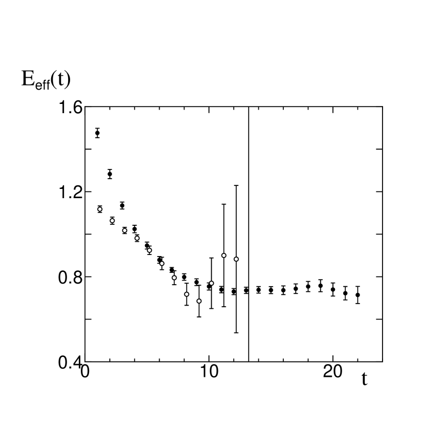
Figure 1: Effective binding energy of the local-local correlation function for $m_{Q}=1000$ (open circles) and $m_{Q}=5$ (filled circles), both with $K=0.1530$ for light quark.

In Fig.1 we plot the effective binding energy defined by

$$E_{eff}(t)=-\log(\frac{C(t+1)}{C(t)}),\quad C(t)=C^{LL}(t)$$ (14)

for $m_{Q}$=1000 (open circles) and 5.0 (filled circles). It is clear that the signal is far better for $m_{Q}$=5.0 for which we find a clear plateau at $t\geq$ 12. It is well known that the signal for the correlation function in the static limit is very noisy, which we also observe here for $m_{Q}=1000$.

The improvement of ground state signals for large but finite values of $m_{Q}$ can be qualitatively understood from the estimate of the relative error[12],

$$\frac{\delta C(t)}{C(t)}\propto\exp\left[\big{(}E(Q\bar{q})-\frac{E(Q\bar{Q})+m_{\pi}}{2}\big{)}t\right]$$ (15)

where $E(Q\bar{q})$ and $E(Q\bar{Q})$ are the binding energies of heavy-light and heavy-heavy mesons respectively. Values of binding energies for $K=0.1530$ are listed in Table 2. For finite $m_{Q}$ the negative contribution from $E(Q\bar{Q})$ significantly reduces the value of the exponential slope from that in the static limit where $E(Q\bar{Q})=0$, leading to a much milder growth of the relative error.

We found that our data for $\delta C(t)/C(t)$ are quantitatively consistent with the above estimate. In Fig.2 we show typical examples of the relative error $\delta C(t)/C(t)$ where solid lines indicate the slope expected from the measured values of the binding energies and $m_{\pi}$ according to (15). Fitting $\delta C(t)/C(t)$ with the exponential function $\exp{(\alpha t)}$ we compare the results for $\alpha$ with the estimate from the binding energies in Table 2. We observe quantitative agreement between $\alpha$ and $E(Q\bar{q})-\frac{E(Q\bar{Q})+m_{\pi}}{2}$ except for a few cases.

3.3 Smearing

In ref.[10] we reported a disappointing fact that the measured values of the heavy-light decay constant in the static limit actually depend on the choice of smearing of the axial vector current. Here we study if this problem is avoided in non-relativistic QCD. We use the cube smearing as a typical choice of the smearing function and examine the dependence of the decay constant on the size of the cube. The smeared current is defined as

$$A^{S}_{\mu}(x)\equiv\frac{1}{n^{3}}\sum_{i}(Q^{\dagger}(x_{i}),0)\gamma_{\mu}\gamma_{5}q(x)$$ (16)

where the sum is over points contained in a cube of a size $n^{3}$ centered at $x$. We employ the Coulomb gauge fixing instead of inserting gauge links between the heavy and light quark fields. We compute the local-smeared (LS) and smeared-smeared (SS) correlation functions defined by

$$C^{LS}(t) \equiv \sum_{x}\langle 0|TA^{L}_{4}(x,t)A^{S}_{4}(0,0)|0\rangle$$ (17)

$$C^{SS}(t) \equiv \sum_{x}\langle 0|TA^{S}_{4}(x,t)A^{S}_{4}(0,0)|0\rangle$$ (18)

for the sizes of smearing $\mbox{3}^{3}$, $\mbox{5}^{3}$, $\mbox{7}^{3}$ and $\mbox{9}^{3}$. Fitting these correlation functions as

$$C^{LS}(t) \longrightarrow Z^{LS}\exp(-Et)$$ (19)

$$\frac{C^{SS}(t)}{C^{LS}(t)} \longrightarrow Z^{S/L}$$ (20)

for large enough $t$ regions, we calculate the heavy-light decay constant using

$$\frac{1}{2}f_{P}^{2}m_{P}=Z_{A}^{2}\frac{Z^{LS}}{Z^{S/L}}$$ (21)

where $Z_{A}$ is the renormalization factor of the lattice axial vector current.

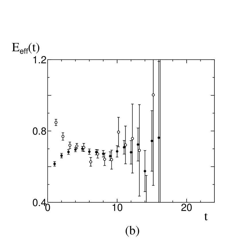
Figure 3: Effective binding energy of the local-smeared (LS) and smeared-smeared(SS) correlation functions for (a) $m_{Q}$=5.0 and (b) $m_{Q}$=1000, both with $K$=0.1530 for light quark. Smearing size is $5^{3}$.

In Fig.3 we plot the effective binding energies of the LS(filled circles) and SS(open circles) correlation functions with the $\mbox{5}^{3}$ smearing. At $m_{Q}$=5.0 (Fig.3(a)) clear signal of the ground state is observed beyond $t\approx$ 10 both for LS and SS correlators. Furthermore the values of the binding energies are consistent. At $m_{Q}$=1000 (Fig.3(b)), on the other hand, it is impossible to identify a plateau.

In Fig.4 we plot the values of $f_{P}\sqrt{m_{P}}/Z_{A}$ extracted from fits of the correlation functions over 4 time slices $t_{min}\leq t\leq t_{max}=t_{min}+4$ for various smearing sizes. For each group of data points $t_{min}$ is taken to be $t_{min}$=6, 8, 10 and 12 from left to right. At $m_{Q}$=5.0 (Fig.4(a)) we observe that the estimates converge to the same value after $t_{min}\sim$ 10 for all the smearing sizes including the case of no smearing (denoted by $1^{3}$ in Fig.4(a)). This gives us confidence that the asymptotic region where the ground state dominates the correlation function is reached at $t\approx$ 10–12. Furthermore it is interesting to notice that the magnitude of errors are similar for various smearing sizes including the case of no smearing. This indicates that the smearing technique does not improve statistics for this case.

At $m_{Q}$=1000 (Fig.4(b)) the situation is quite different. Here only results for $t_{min}$=6 and 8 are available because of rapid growth of noise at $t>$ 10. For these fitting intervals the data still depend on the size of smearing, showing that the asymptotic region is not yet reached. It is essential for calculations in the static limit to use some method which enhance ground state signals in the region $t<$ 10. We do not use the data at $m_{Q}$=1000 in the following analysis.

3.4 Decay Constant

Because the results for the decay constant for $m_{Q}\leq$ 10.0 do not depend on the smearing size for $t_{min}\geq$ 10, we choose the cube smearing of size $\mbox{5}^{3}$ and extract $f_{P}\sqrt{m_{P}}/Z_{A}$ from a global fit over the interval 10 $\leq t\leq$ 20. Other choices give similar results.

In Table 3 we summarize our results for the binding energy $E$ and the decay constant $f_{P}\sqrt{m_{P}}/Z_{A}$ at each value of the hopping parameter of light quark $K$ and the heavy quark mass $m_{Q}$. Errors are estimated by the single elimination jackknife procedure. We observe that the two actions with $n=1$ and 2 yield consistent values for $f_{P}\sqrt{m_{P}}/Z_{A}$ for $m_{Q}=4.0$ and 5.0 where both actions are employed. For each $m_{Q}$ we extrapolate the results at three values of $K$ linearly in $1/K$ to $1/K_{c}$ (see Fig.5), the results of which are also given in Table 3.

4 Extracting Physical Value of $f_{B}$

In order to estimate the physical value of the $B$ meson decay constant $f_{B}$ we have to determine the heavy quark mass $m_{Q}$ corresponding to the $b$ quark and the renormalization factor of the axial vector current $Z_{A}$. A complete one-loop perturbative calculation necessary for this purpose is not yet available for our non-relativistic QCD action (4) with $c$=1. Davies and Thacker[21, 22], however, have reported the one-loop results for the case of $c$=0, and we use their results incorporating the tadpole improvement of lattice perturbation theory [23].

4.1 Improved Perturbation Theory for Non-relativistic QCD

To one-loop order the inverse heavy quark propagator $\Delta_{Q}$ can be written in the form,

$$\Delta_{Q}=(1-Cg^{2})\left[(e^{ip_{0}}-1-Ag^{2})+(1-Bg^{2})\frac{\mbox{\bf p}^{2}}{2m_{Q}}\right]$$ (22)

where $A$, $B$ and $C$ are numerical constants. We define the mass renormalizaion factor $Z_{m}$, the energy shift $E_{0}$ and the wave function renormalization factor $Z_{Q}$ by

$$G^{pert}(\mbox{\bf p},t) = \int^{+\pi}_{-\pi}\frac{dp_{0}}{2\pi}\frac{1}{\Delta_{Q}}e^{ip_{0}t}$$

$$= \frac{1}{1-Cg^{2}}\left[(1+Ag^{2})-(1-Bg^{2})\frac{\mbox{\bf p}^{2}}{2m_{Q}}\right]^{t-1}$$

$$\equiv Z_{Q}^{pert}\exp\left[-t\left(E_{0}^{pert}+\frac{\mbox{\bf p}^{2}}{2Z_{m}^{pert}m_{Q}}\right)\right].$$

We then obtain

$$E_{0}^{pert} = -\ln[1+Ag^{2}]$$

$$Z_{m}^{pert} = 1+(A+B)g^{2}$$

$$Z_{Q}^{pert} = \frac{1}{1-(C-A)g^{2}}.$$ (24)

For these quantities the mean-field improved[23] expressions are given by

$$E_{0}^{mf} = -\ln\left[u_{0}\left(1-\frac{3}{nm_{Q}}(1-u_{0})\right)^{n}\right]$$

$$Z_{m}^{mf} = \frac{1}{u_{0}}\left(1-\frac{3}{nm_{Q}}(1-u_{0})\right)$$

$$Z_{Q}^{mf} = \frac{1}{\left(1-\frac{3}{nm_{Q}}(1-u_{0})\right)^{n}}$$ (25)

where $u_{0}$ is a mean-field value of the lattice link variable $U_{\mu}(x)$. As a definition of $u_{0}$ we take the simplest choice $u_{0}=\langle\frac{1}{3}\mbox{Tr}U_{plaq}\rangle^{1/4}$ for which the perturbative expansion is given by $u_{0}^{pert}=1-\frac{1}{12}g^{2}$.

Tadpole-improved one-loop results for the renormalization factors are obtained by combining (25) and (24) after removing one-loop terms of the mean-field expressions (25) from $A,B$ and $C$. This gives

$$E_{0}^{tad-imp} = -\ln\left[u_{0}\left(1-\frac{3}{nm_{Q}}(1-u_{0})\right)^{n}\left\{1+\tilde{A}g^{2}\right\}\right]$$

$$Z_{m}^{tad-imp} = \frac{1}{u_{0}}\left(1-\frac{3}{nm_{Q}}(1-u_{0})\right)\left\{1+\widetilde{(A+B)}g^{2}\right\}$$

$$Z_{Q}^{tad-imp} = \frac{1}{\left(1-\frac{3}{nm_{Q}}(1-u_{0})\right)^{n}}\left\{1+\widetilde{(C-A)}g^{2}\right\}.$$ (26)

where $\tilde{A}$, $\widetilde{(A+B)}$, $\widetilde{(C-A)}$ are again numerical constants defined by

$$\tilde{A} = A+\frac{1}{12}\left(1+\frac{3}{m_{Q}}\right)$$

$$\widetilde{(A+B)} = (A+B)-\frac{1}{12}\left(1-\frac{3}{nm_{Q}}\right)$$

$$\widetilde{(C-A)} = (C-A)-\frac{1}{4m_{Q}}.$$ (27)

In Table 4 we summarize numerical values of these quantities for some typical values of $m_{Q}$ where we use the values obtained by Davies and Thacker for the numerical coefficients $A$, $B$ and $C$. Smallness of the ‘tilde’ quantities compared with the original values demonstrates that the tadpole improvement works well for these quantities.

The values of $E_{0},Z_{m}$ and $Z_{Q}$ are also tabulated in Table 4. For the coupling constant $g^{2}$ we take $g_{V}^{2}(\pi/a)=1.96$ at $\beta=6.0$[23]. In principle it is more desirable to use $g_{V}^{2}(q^{\ast})$ with a properly determined scale $q^{\ast}$ as proposed in [23]. Morningstar has calculated this scale $q^{\ast}$ for a more complicated non-relativistic QCD action[24] and obtained $q^{\ast}$=0.67$a^{-1}$ for $Z_{m}$ and 0.81$a^{-1}$ for $E_{0}$. The corresponding values of $g_{V}^{2}(q^{\ast})$ (it e.g., $g_{V}^{2}(0.67/a)=3.41$) are substantially larger than $g_{V}^{2}(\pi/a)$. Because of the smallness of the tadpole-improved one-loop coefficients, however, the renormalization constants are modified only slightly; the combination $Z_{m}m_{Q}-E_{0}$ which is relevant for the $B$ meson mass (see below) changes only by 2–3%, and the change of the heavy quark wave function renormalization factor $Z_{Q}$ is also at the level of a few percent.

4.2 $b$ Quark Mass

The heavy-light meson mass is given by

$$m_{P}=Z_{m}m_{Q}-E_{0}+E_{Q\bar{q}}.$$ (28)

In Fig. 6 we plot our numerical result for the binding energy $E_{Q\bar{q}}$ as a function of $1/m_{Q}$. The solid line $E_{Q\bar{q}}=\mbox{0.60}+\mbox{0.33}/m_{Q}$ fits the data very well. Using this fit and the perturbative result for $Z_{m}$ and $E_{0}$ discussed in Sec. 4.1, together with the inverse lattice spacing $a^{-1}$ = 2.3(3) GeV obtained from the $\rho$ meson mass, we find $m_{P}$ = 12.6(1.6), 7.2(9) and 5.4(7) GeV for $m_{Q}$ = 5.0, 2.5 and 1.8 respectively. This shows that the heavy quark mass of $m_{Q}$ = 1.8 in lattice units approximately corresponds to the $b$ quark. This value is consistent with the estimate given by Davies and Thacker using $\Upsilon$ spectroscopy[25]. In the following analysis of the $B$ meson decay constant we use $m_{Q}$ = 1.8 for the $b$ quark mass.

4.3 Axial vector current renormalization factor $Z_{A}$

The renormalization factor $Z_{A}$ for the axial vector current can be written as

$$Z_{A}=\frac{Z_{A}^{cont}}{Z_{A}^{latt}}.$$ (29)

Here $Z_{A}^{cont}$ is the renormalization constant for the continuum axial vector current renormalized with the $\overline{\mbox{MS}}$ scheme[26] given by

$$Z_{A}^{cont}=1+\frac{1}{12\pi^{2}}g^{2}\left(\frac{3}{2}\log(m_{Q}^{cont})^{2}-\frac{3}{4}\right)$$ (30)

where we use $m_{Q}^{cont}=Z_{m}m_{Q}$ as the heavy quark mass. We ignore infra-red divergent logarithms since it cancels with the lattice counterpart. The lattice renormalization factor $Z_{A}^{latt}$ can be written as

$$Z_{A}^{latt}=Z_{Q}^{1/2}Z_{q}^{1/2}[1+V^{latt}g^{2}]$$ (31)

where $Z_{Q}$ is the wave function renormalization factor for the heavy quark discussed in Sec. 4.1. For the Wilson light quark our field normalization includes the conventional factor $\sqrt{2K_{c}}$. The tadpole-improved one-loop result for the wave function renormalization factor $Z_{q}$ is then given by[23]

$$Z_{q}=\frac{2K_{c}}{1/4}[1+0.0043g^{2}].$$ (32)

Finally the vertex correction $V^{latt}$ is not affected by the tadpole improvement. We use the value given in ref. [22] for the spinless non-relativistic QCD action ($c$=0) since theirs is the only result available for this quantity at present. Combining these quantities we obtain the final expression,

$$Z_{A} = \left(1-\frac{3}{nm_{Q}}(1-u_{0})\right)^{n/2}\left(\frac{1/4}{2\kappa_{c}}\right)^{1/2}$$

$$\times\left[1-\left(\tilde{D}-\frac{1}{4\pi^{2}}\ln(m_{Q}^{cont}a)\right)g^{2}\right]$$

where $\tilde{D}$ is a numerical constant.

In Table 5 we list representative values of $V^{latt},\tilde{D},1/Z_{A}^{latt}$ and $Z_{A}$. It is interesting to note that the value of $Z_{A}^{latt}$ is almost independent of $1/m_{Q}$ while $Z_{A}$ shows logarithmistic dependence and even diverges at $m_{Q}=\infty$ reflecting the form of $Z_{A}^{cont}$ (eq.(30)). We also observe that the expansion coefficient $\tilde{D}$ is still large after the tadpole improvement, suggesting the possibility that higher order coefficients may not be small[4]. The main contribution to the large coefficient is the vertex correction $V^{latt}$ which is unmodified by the tadpole improvement. This is a general feature for renormalization constants of bilinear operators of light-light, heavy-light and heavy-heavy quarks.

The large one-loop coefficient increases the magnitude of uncertainties coming from the choice of the scale $q^{\ast}$ in the coupling constant $g_{V}^{2}(q^{\ast})$. In the static limit, the optimal value of $q^{\ast}$ is estimated[27] as $q^{\ast}=2.18/a$ for which $g_{V}^{2}(q^{\ast})$=2.22 at $\beta=6.0$. This choice of $q^{\ast}$ leads to $Z_{A}$=0.661 at $m_{Q}=\infty$, while another choice $q^{\ast}=1/a$ for which $g_{V}^{2}(q^{\ast})$=3.10 gives $Z_{A}$=0.570 which is 14 % smaller. In the following we use $q^{\ast}=2.18/a$ for a reference value, keeping in mind this large systematic uncertainty.

4.4 Decay Constant

Our results for $f_{P}\sqrt{m_{P}}/Z_{A}$ after extrapolation to $K=K_{c}$ for light quark are plotted as a function of $1/m_{Q}$ in Fig.7 (see Table 3 for numerical values). Circles and triangles are for the results obtained with the $n=1$ and $2$ actions respectively. The two actions yield consistent values for $m_{Q}=4.0$ and 5.0 as we already noted in Sec. 3.4.

We observe in Fig. 7 a clear deviation from the scaling law of the heavy-light decay constant in the heavy mass limit given by

$$f_{P}\sqrt{m_{P}}/Z_{A}=\mbox{const}.$$ (34)

In order to evaluate the magnitude of the deviation we fit the data with the form

$$f_{P}\sqrt{m_{P}}/Z_{A}=(f_{P}\sqrt{m_{P}}/Z_{A})^{static}\left(1-\frac{c}{m_{Q}}\right).$$ (35)

In order to estimate systematic uncertainties in the fit due to a slight curvature in the $1/m_{Q}$ dependence of $f_{P}\sqrt{m_{P}}/Z_{A}$, we list in Table 6 the results of fit for four representative selection of data points. The first two choices employ all data points except at $m_{Q}=4.0$ and 5.0 where the results with the $n=2$ action is chosen for the choice (a) and those with the $n=1$ action for the choice (b). The choice (c) uses data for $5.0\geq m_{Q}\geq 2.5$ with the $n=2$ action and (d) for $10.0\geq m_{Q}\geq 4.0$ with $n=1$. Errors given in Table 6 are estimated by a single elimination jackknife procedure.

For the decay constant in the static limit $(f_{P}\sqrt{m_{P}}/Z_{A})^{static}$ all four choices yield values consistent within 10–15%. As a representative value we quote the result for the choice (a);

$$(f_{P}\sqrt{m_{P}}/Z_{A})^{static}=\mbox{0.292(35),\hskip 28.45274pt}c=\mbox{1.04(44)}$$ (36)

The extrapolated value (36) is compared with the results of other groups obtained at $\beta=6.0$ using the static heavy quark propagator in Table 7. The results are consistent in view of the systematic uncertainties in the static results depending on the detail of smearing.

Using the value (36) for $(f_{P}\sqrt{m_{P}}/Z_{A})^{static}$ we obtain the heavy-light decay constant in the static limit,

$$(f_{P}\sqrt{m_{P}})^{static}=0.682\pm 82^{+34}_{-70}\left(\frac{Z_{A}}{0.67}\right)\left(\frac{a^{-1}}{2.3\mbox{GeV}}\right)^{3/2}\mbox{GeV}^{3/2}$$ (37)

where the first error is statistical and the second one is systematic reflecting variation of central values among the four selection of data points in Table 6. For the renormalization factor of the axial current $Z_{A}$ which diverges in this limit we use the value evaluated at the $b$-quark mass as a normalization as usual. For the $B$ meson decay constant evaluated in the static limit this yields

$$f_{B}^{static}=297\pm 36^{+15}_{-30}\left(\frac{Z_{A}}{0.67}\right)\left(\frac{a^{-1}}{2.3\mbox{GeV}}\right)\mbox{MeV}.$$ (38)

In order to obtain the $B$ meson decay constant including $1/m_{Q}$ corrections we extrapolate the fit (35) to the $b$ quark mass of $m_{Q}$=1.8 as was discussed in Sec.4.2, employing the single elimination jackknife procedure for estimating the statistical error of the extrapolated value. The result shows a sizable variation depending on the selection of data points. We quote the value for the fitting choice (d) in Table 6 employing data for $5.0\geq m_{Q}\geq 2.5$, which are close to the extrapolated point $m_{Q}=1.8$ and hence should be more reliable;

$$f_{B}=171\pm 22^{+19}_{-45}\left(\frac{Z_{A}}{0.67}\right)\left(\frac{a^{-1}}{2.3\mbox{GeV}}\right)\mbox{MeV}.$$ (39)

where the first error is statistical and the second one is systematic showing the uncertainty originating from the choice of data points for the fitting. It should be remembered that a systematic uncertainty also exists in the determination of $Z_{A}$ and $a^{-1}$.

The UKQCD collaboration[28] recently reported a preliminary non-relativistic QCD result for $f_{B}$ obtained in a simulation carried out at $m_{Q}=1.7$ on a $16^{3}\times 48$ lattice. Their result $f_{B}\sqrt{m_{B}}/Z_{A}=0.16(3)$ is consistent with our value obtained by an extrapolation in $1/m_{Q}$.

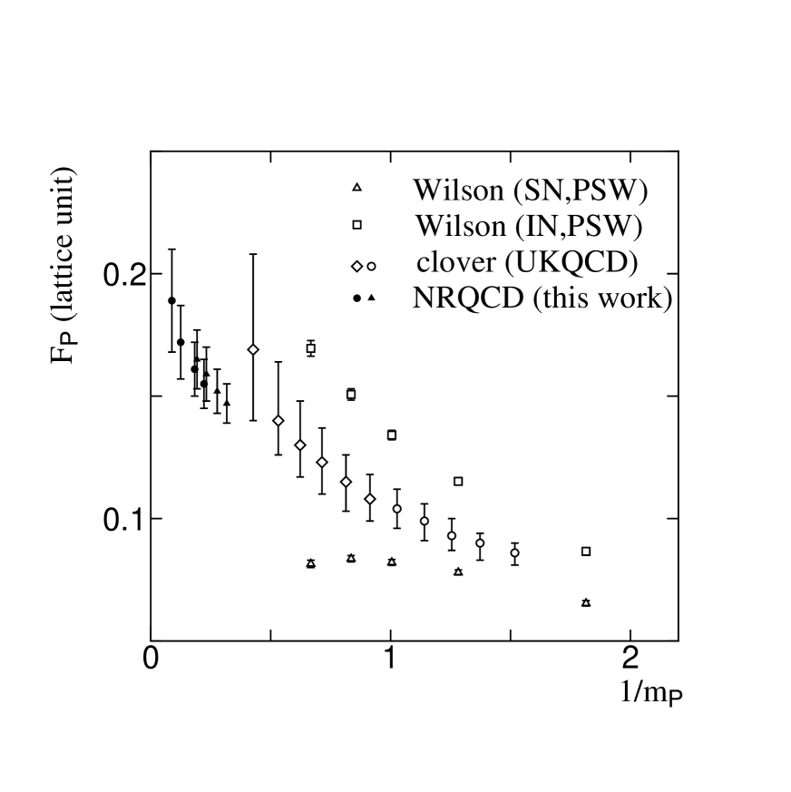
Figure 8: $F_{P}=(\alpha_{s}(m_{P})/\alpha_{s}(m_{B}))^{2/11}f_{P}\sqrt{m_{P}}$ as a function of $1/m_{P}$ after the extrapolation to the limit $K=K_{c}$ for light quark. Open squares and tringles are for results of the PSI-Wuppertal collaboration[29] using the Wilson action with the standard normalization $\sqrt{2K}$ (triangles) and with the improved normalization $\sqrt{1-3K/4K_{c}}$ (squares). Open circles and diamonds are for results of the UKQCD collaboration[20] using the $O(a)$-improved (clover) fermion action. Closed symbols are for results of this work.

It is also interesting to compare our results with the results obtained using propagating quark for the heavy quark. Two groups have reported the results of $f_{P}\sqrt{m_{P}}$ obtained using the propagating quarks at $\beta=$6.0. In Fig.8 we plot the quantity

$$F_{P}=\left(\frac{\alpha_{s}(m_{P})}{\alpha_{s}(m_{B})}\right)^{2/11}f_{P}\sqrt{m_{P}}$$ (40)

as a function of $1/m_{P}$. The normalization factor $(\alpha_{s}(m_{P})/\alpha_{s}(m_{B}))^{2/11}$ is introduced in order to absorb the logarithmistic divergence of $f_{P}\sqrt{m_{P}}$ at $m_{P}=\infty$ originating from $Z_{A}^{cont}$ (eq.(30)). As a coupling constant we use $\alpha_{V}$ with $\Lambda_{V}$=0.169 at $\beta$=6.0. Open squares and tringles are for results of the PSI-Wuppertal collaboration[29] using the Wilson action with the standard normalization $\sqrt{2K}$ (triangles) and with the improved normalization $\sqrt{1-3K/4K_{c}}$ (squares). Open circles and diamonds are for results of the UKQCD collaboration[20] using the $O(a)$-improved (clover) fermion action. Closed symbols are for results of this work. We can see that our results are consistent with the results of the clover action in view of the $1/m_{P}$ dependence of $F_{P}$. For the Wilson action there is a source of large systematic uncertainty in the choice of the normalization for this heavy mass region and our results are not seen to be consistent with both of these choices.

5 Conclusions

In this article we have reported on a calculation of the heavy-light decay constant using non-relativistic lattice QCD. We found that ground state signals in the correlator is significantly improved compared to those in the static limit, and that the degree of improvement of signal to noise ratio is in a quantitative agreement with the estimate of Lepage in terms of binding energies. As a result we could extract properties of the ground state reliably. In particular an apparent dependence of the decay constant on the size of smearing for source, which affected previous attempts in the static limit, is absent.

Our result for the $B$ meson decay constant shows that the $1/m_{Q}$ correction to the static limit is quite significant even for the $b$ quark. This points toward the necessity of a more complete calculation to order $1/m_{Q}$ than was attempted here, and eventually a calculation including $1/m_{Q}^{2}$ terms, for a precise determination of the $B$ meson decay constant. The improvements of the present work needed to order $1/m_{Q}$ are the inclusion of $1/m_{Q}$ terms in the axial vector current and one-loop calculation of renormalization factors including the spin-magnetic interaction. It is also desirable to estimate two-loop vertex corrections in view of the large one-loop coefficient. We leave these problems for future investigations.

$K$	$m_{\pi}$	$m_{\rho}$	$f_{\pi}/Z_{A}$
0.1530	0.419(4)	0.502(12)	0.105(4)
0.1540	0.360(5)	0.461(14)	0.096(5)
0.1550	0.291(7)	0.416(21)	0.081(6)
$K_{c}$	0	0.338(40)	0.067(11)

Table 1: $\pi$ and $\rho$ meson masses and the pion decay constant $f_{\pi}$ devided by the renormalization constant of the axial current in lattice units. The values of $m_{\rho}$ and $f_{\pi}/Z_{A}$ at the critical hopping parameter are obtained by a linear extrapolation in $1/K$.

$m_{Q}$	$E(Q\bar{q})$	$E(Q\bar{Q})$	$E(Q\bar{q})-\frac{E(Q\bar{Q})+m_{\pi}}{2}$	$\alpha$
1000	0.647(18)	0	0.438(18)	0.466(10)
10.0	0.713(24)	0.510(08)	0.249(24)	0.155(51)
7.0	0.720(16)	0.638(12)	0.192(17)	0.153(30)
5.0($n$=1)	0.740(14)	0.751(12)	0.155(15)	0.149(22)
5.0($n$=2)	0.738(13)	0.729(13)	0.164(15)	0.147(24)
4.0($n$=1)	0.759(14)	0.827(11)	0.136(15)	0.125(22)
4.0($n$=2)	0.756(12)	0.804(09)	0.145(13)	0.138(22)
3.0	0.786(12)	0.906(14)	0.124(14)	0.116(23)
2.5	0.810(15)	0.977(14)	0.112(17)	0.101(23)

Table 2: The heavy-light and heavy-heavy binding energies $E(Q\bar{q})$ and $E(Q\bar{Q})$ at $K$=0.1530 for the light quark. The combination $E(Q\bar{q})-\frac{E(Q\bar{Q})+m_{\pi}}{2}$ determines the behavior of the noise (see Eq.(15) in text). $\alpha$ denotes the measured value of the exponential slope.

Binding energy $E$
$m_{Q}$	$K$= 0.1530	0.1540	0.1550	$K_{c}$=0.157
10.0	0.696(15)	0.681(15)	0.668(17)	0.640(21)
7.0	0.711(14)	0.695(13)	0.679(16)	0.647(18)
5.0
($n$=1)	0.734(12)	0.717(14)	0.700(14)	0.666(15)
($n$=2)	0.732(12)	0.714(14)	0.698(14)	0.665(15)
4.0
($n$=1)	0.755(13)	0.737(12)	0.720(14)	0.685(12)
($n$=2)	0.750(12)	0.733(15)	0.716(13)	0.682(15)
3.0	0.781(15)	0.763(14)	0.746(13)	0.711(13)
2.5	0.806(13)	0.788(13)	0.770(12)	0.735(15)

Decay constant $f_{P}\sqrt{m_{P}}/Z_{A}$
$m_{Q}$	0.1530	0.1540	0.1550	$K_{c}$=0.157
10.0	0.346(19)	0.329(20)	0.314(24)	0.282(32)
7.0	0.328(14)	0.310(15)	0.292(17)	0.257(22)
5.0
($n$=1)	0.313(11)	0.294(12)	0.276(13)	0.241(17)
($n$=2)	0.319(12)	0.300(13)	0.282(14)	0.246(18)
4.0
($n$=1)	0.302(10)	0.284(11)	0.266(12)	0.232(15)
($n$=2)	0.309(11)	0.291(11)	0.272(13)	0.237(16)
3.0	0.295(09)	0.278(10)	0.261(11)	0.227(14)
2.5	0.287(09)	0.270(09)	0.253(10)	0.220(12)

Table 3: Binding energy $E$ and decay constant $f_{P}\sqrt{m_{P}}/Z_{A}$ at $K$=0.1530, 0.1540, 0.1550. Values at $K_{c}$=0.15708(2) are obtained by a linear extrapolation in $1/K$.

$E_{0}$
$m_{Q}$	$A$	$\widetilde{A}$	$E_{0}^{pert}$	$E_{0}^{mf}$	$E_{0}^{tad-imp}$
$\infty$	-0.1684	-0.0851	0.401	0.129	0.310
5.0	-0.2075	-0.0742	0.522	0.202	0.359
2.5	-0.2487	-0.0654	0.668	0.277	0.414
1.8	-0.2809	-0.0586	0.800	0.338	0.460

$Z_{m}$
$m_{Q}$	$A+B$	$\widetilde{A+B}$	$Z_{m}^{pert}$	$Z_{m}^{mf}$	$Z_{m}^{tad-imp}$
$\infty$	0.0686	-0.0147	1.13	1.14	1.11
5.0	0.0434	-0.0101	1.09	1.05	1.03
2.5	0.0707	0.0374	1.14	1.05	1.13
1.8	0.0675	0.0536	1.13	1.02	1.13

$Z_{Q}$
$m_{Q}$	$C-A$	$\widetilde{C-A}$	$Z_{Q}^{pert}$	$Z_{Q}^{mf}$	$Z_{Q}^{tad-imp}$
$\infty$	0.0383	0.0383	1.075	1.000	1.075
5.0	0.0673	0.0173	1.132	1.077	1.114
2.5	0.1003	0.0003	1.197	1.161	1.162
1.8	0.1268	-0.0121	1.249	1.235	1.206

Table 4: Renormalization parameters for non-relativistic QCD. The $n$=1 action is used at $m_{Q}$=$\infty$ and 5.0 while the $n$=2 action is used at 2.5 and 1.8. As the coupling constant we use $g_{V}^{2}(\pi/a)$=1.96 at $\beta$=6.0.

$Z_{A}$
$m_{Q}$	$V^{latt}$	$\tilde{D}$	$1/Z_{A}^{latt}$	$Z_{A}$
$\infty$	0.1070	0.1346	0.638	$\infty$
5.0	0.0972	0.1143	0.654	0.721
2.5	0.0920	0.1006	0.655	0.692
1.8	0.0897	0.0921	0.650	0.671

Table 5: Renormalization factors for the heavy-light axial vector current. As a coupling constant we use $g_{V}^{2}(2.18/a)$=2.22[27] at $\beta$=6.0.

	$m_{Q},n$	$(f_{P}\sqrt{m_{P}}/Z_{A})^{static}$	$c$	$f_{B}\sqrt{m_{B}}/Z_{A}$
(a)	10.0, 7.0 ($n$=1) and 5.0, 4.0, 3.0, 2.5 ($n$=2)	0.292(35)	1.04(35)	0.124(44)
(b)	10.0, 7.0, 5.0, 4.0 ($n$=1) and 3.0, 2.5 ($n$=2)	0.284(31)	0.61(21)	0.187(19)
(c)	10.0, 7.0, 5.0, 4.0 ($n$=1)	0.307(44)	1.03(44)	0.132(52)
(d)	5.0, 4.0, 3.0, 2.5 ($n$=2)	0.262(22)	0.64(21)	0.168(22)

Table 6: Results of fitting with the form (35) in the text and the value of $f_{P}\sqrt{m_{P}}/Z_{A}$ at $m_{Q}=1.8$ (last column). (a), (b), (c) and (d) label the selection of data points.

Group	Lattice	Smearing	$(f_{P}\sqrt{m_{P}}/Z_{A})^{static}$
APE[17]	$\mbox{18}^{3}\times\mbox{32}$	cube, $n$=5	0.368(14)
		$n$=7	0.311(14)
Bernard et al.[18]	$\mbox{24}^{3}\times\mbox{39}$	cube, $n$=5	0.369(18)
		$n$=7	0.299(10)
		$n$=9	0.241(12)
PSI-Wuppertal[19]	$\mbox{12}^{3}\times\mbox{36}$	exponential, gaussian	0.327(14)
UKQCD[20]	$\mbox{16}^{3}\times\mbox{48}$	Jacobi	0.298(10)
this work	$\mbox{16}^{3}\times\mbox{48}$	independent (see text.)	0.292(35)

Table 7: Comparison of results for $(f_{P}\sqrt{m_{P}}/Z_{A})^{static}$ obtained by several groups at $\beta$=6.0.

Figure 2: Relative error of local-local correlation function for $m_{Q}=1000$ (open circles) and $m_{Q}=5$ (filled circles), both with $K=0.1530$ for light quark. Solid lines indicate the slope expected from measured values of the binding energies and $m_{\pi}$ according to (15).

Figure 4: Dependence of $f_{P}\sqrt{m_{P}}/Z_{A}$ on the fitting range $t_{min}<t<t_{min}+\mbox{4}$ for various smearing sizes at $m_{Q}=$1000 (a) and $m_{Q}=$5.0 (b) with $K$=0.1530 for light quark.

Figure 5: $f_{P}\sqrt{m_{P}}/Z_{A}$ as a function of $1/2K$ for $m_{Q}$=10.0 (circles), 5.0 (squares) and 2.5 (diamonds). The solid line indicates the extrapolation to the chiral limit $1/2K_{c}$.

Figure 6: The binding energy $E_{Q\bar{q}}$ of the heavy-light meson as a function of $1/m_{Q}$ Circles and triangles are for the results obtained with the $n$=1 and $n$=2 actions respectively. The solid line represents the fit $E_{Q\bar{q}}=\mbox{0.60}+\mbox{0.33}/m_{Q}$.

Figure 7: $1/m_{Q}$ dependence of $f_{P}\sqrt{m_{P}}/Z_{A}$ after the extrapolation to the limit $K=K_{c}$ for light quark. Circles and triangles are for the results obtained with the $n$=1 and $n$=2 actions respectively.

References

- [1] For a recent review, see B. Grinstein, and M. Neubert, SLAC-PUB-6263 (1993).
- [2] E. Eichten, in “Field Theory on the Lattice”, Nucl. Phys. B (Proc. Suppl.) 4 (1988) 147.
- [3] G.P. Lepage and B. Thacker, ibid, 199.
- [4] For a recent review, see C.W. Bernard, review at lattice 93 to appear in the proceedings, hep-lat.9312086.
- [5] Ph. Boucaud et al., Phys. Lett. B220 (1989) 219.
- [6] C. Alexandrou, F. Jegerlehner, S. Güsken, K. Schilling and R. Sommer, Phys. Lett. B256 (1991) 60.
- [7] C.R. Allton, C.T. Sachrajda, V. Lubicz, L. Maiani and G. Martinelli, Nucl. Phys. B349 (1991) 598.
- [8] E. Eichten, G. Hockney and H.B. Thacker, in Lattice 90, Nucl. Phys. B (Proc. Suppl.) 20 (1990) 500.
- [9] C. Bernard, J. Labrenz and A. Soni, Nucl. Phys. B (Proc. Suppl.) 20 (1990) 488.
- [10] S. Hashimoto and Y. Saeki, Mod. Phys. Lett. A7 (1992) 387.
- [11] C. Bernard, C.M. Heard, J. Labrenz and A. Soni, Nucl. Phys. B (Proc. Suppl.) 26 (1992) 384.
- [12] G.P. Lepage, in “Lattice 91”, Nucl. Phys. B (Proc. Suppl.) 26 (1991) 45.
- [13] B.A. Thacker and G.P. Lepage, Phys. Rev. D43 (1991) 196.
- [14] G.P. Lepage et al., Phys. Rev. D46 (1992) 4052.
- [15] N. Cabbibo and E. Marinari, Phys. Lett. B119 (1982) 387; M. Okawa, Phys. Rev. Lett. 49 (1982) 353.
- [16] G. Martinelli and Y.C. Zhang, Phys. Lett. B123 (1983) 433.
- [17] APE collaboration, Nucl. Phys. B (Proc. Suppl.) 30 (1993) 469.
- [18] C.W. Bernard, J.N. Labrenz and A. Soni, preprint UW/PT-93-06, hep-lat.9306009.
- [19] C. Alexandrou, S. Güsken, F. Jegerlehner, K. Schilling and R. Sommer, preprint CERN-TH 6692/92, hep-lat.9211042.
- [20] UKQCD collaboration, Phys. Rev. D49 (1994) 1594.
- [21] C.T.H. Davies and B.A. Thacker, Phys. Rev. D45 (1992) 915.
- [22] C.T.H. Davies and B.A. Thacker, Phys. Rev. D48 (1993) 1329.
- [23] G.P. Lepage and P.B. Mackenzie, Phys. Rev. D48 (1993) 2250.
- [24] C.J. Morningstar, talk at Lattice 93 to appear in the proceedings, hep-lat.9311034.
- [25] C.T.H. Davies and B.A. Thacker, Nucl. Phys. B405 (1993) 593.
- [26] See, for example, E. Eichten and B. Hill, Phys. Lett. B234 (1990) 511.
- [27] O.F. Hernández and B.R. Hill, preprint hep-lat.9401035.
- [28] UKQCD collaboration, C.T.H. Davies, talk at Lattice 93 to appear in the proceedings, hep-lat.9312020.
- [29] C. Alexandrou, S. Güsken, F. Jegerlehner, K. Schilling, G. Siegert and R. Sommer, preprint DESY 93-179, hep-lat.9312051.