UTHEP-257

Interface tension in SU(3) lattice gauge theory at finite temperatures on an $N_{t}=2$ lattice

Yasumichi Aoki and Kazuyuki Kanaya

Institute of Physics, University of Tsukuba,

Tsukuba, Ibaraki 305, Japan

The surface tension $\sigma$ of the confined-deconfined interface is calculated in pure $SU(3)$ lattice gauge theory at finite temperatures employing the operator and integral methods on a lattice of a size $8^{2}\times N_{z}\times 2$ with $N_{z}=16$ and 40. Analyses of non-perturbative corrections in asymmetry response functions strongly indicate that the use of one-loop values for the response functions lead to an overestimate of $\sigma$ in the operator method. The operator method also suffers more from finite-size effects due to a finite thickness of the interface, leading us to conclude that the integral method yields more reliable values for $\sigma$. Our result with the integral method $\sigma/T_{c}^{3}=0.134(16)$ is consistent with earlier results and also with that obtained with a transfer matrix method. Result is also reported on $\sigma$ obtained on a lattice $18^{2}\times 48\times 4$ with the integral method.

1 Introduction

Numerical simulation of pure $SU(3)$ gauge system on a lattice has shown that the system undergoes a first order phase transition from a confined phase at low temperatures to a deconfined phase at high temperatures [1]. The two phases can therefore coexist at the transition temperature $T_{c}$, separated by an interface.

A basic parameter characterizing the interface is the interface tension $\sigma$. A number of numerical work has recently been carried out to determine its value, mainly for a system with the temporal lattice size $N_{t}=2$. Kajantie, Kärkkäinen and Rummukainen[2, 3] developed an operator method for measuring the tension and reported the value $\sigma/T_{c}^{3}=0.24(6)$ for $N_{t}=2$[3]. Independently, Potvin and Rebbi[4] proposed to employ an integral of the derivative of the free energy in the parameter space of the coupling constant to measure the tension, and found $\sigma/T_{c}^{3}=0.115(13)$ for the same temporal lattice size[5]. A factor two discrepancy between these results has motivated further studies of the interface[6, 7, 8, 9], which yielded values of $\sigma/T_{c}^{3}$ similar to that of the integral method. The method of histograms[10] and the technique of transfer matrix[6] used in these studies are quite different, however, from the operator and the integral method. Hence the discrepancy of the original results obtained with the two methods has not been resolved.

In this article we report on our attempt toward an understanding of the origin of the discrepancy through a comparative study of the two methods. Since a possible cause of the discrepancy is the use of a different spatial lattice size ($8^{2}\times 40\times 2$ for the operator method[3] and $8^{2}\times 16\times 2$ for the integral method[5] ), we carry out simulations for both sizes of lattice with both methods. We also increase statistics by a factor of two to four over those of ref. [3, 5]. We find that a part of the discrepancy can be understood by the effect of the finite thickness of the interface. Comparing the results on a large lattice with $N_{z}=40$, where this problem is absent, we find, however that the discrepancy is not completely removed for $N_{t}=2$.

A nice feature of the integral method is that it directly relates plaquette expectation values to the interface tension and no other input is needed. In contrast the operator method requires the values of response functions of the coupling constant under an anisotropic deformation of lattice. Up to now they have been estimated only in one-loop perturbation theory[11], whose applicability may be questioned for small values of the inverse gauge coupling constant $\beta=6/g^{2}$, such as the critical value $\beta_{c}$ for $N_{t}=2$. We discuss the effect of nonperturbative corrections to these coefficients.

Another problem which became apparent in recent work on the interface tension is the difficulty of measuring its value for lattices with the temporal size $N_{t}\geq 4$. For the case of $N_{t}=4$ an initial attempt with the integral method failed to obtain a non-vanishing value[5]. An alternative integral method employing an external field coupled to the Polyakov loop was then devised, and a value $\sigma/T_{c}=0.027(4)$ has been obtained[12]. We attempt a high statistics measurement of the interface tension with the original integral method on a $18^{2}\times 48\times 4$ lattice. The results will also be reported in this article.

This paper is organized as follows. In Sec. 2 we briefly recall the operator and the integral method and describe our simulations. Our results for the interface tension are presented in Sects. 3 and 4 for $N_{t}=2$ and 4, respectively. Sec. 5 is devoted to conclusions.

2 Method and simulation

We consider the pure $SU(3)$ gauge system with the standard plaquette action on a lattice of a size $N_{x}\times N_{y}\times N_{z}\times N_{t}$ with the size $N_{z}$ in the $z$-direction at least twice as large as those in the $x$- and $y$-directions. If one splits the lattice into two halves in the $z$-direction and chooses $\beta$ in one half of the lattice to be slightly below the critical value $\beta_{1}=\beta_{-}\equiv\beta_{c}-\delta\beta$ and that of the other half slightly above $\beta_{2}=\beta_{+}\equiv\beta_{c}+\delta\beta$, the system in the first half will be in the confined phase and the other half in the deconfined phase. With the periodic boundary condition employed for the gauge field in all four directions, there will be two interfaces in the $x-y$ plane, each with a transverse area $A=N_{x}N_{y}a^{2}$ with $a$ the lattice spacing.

The operator method[2, 3] starts from the following thermodynamic relation defining the interface tension $\sigma$ in terms of the free energy $F$,

$$\sigma=\left.\frac{1}{2}\frac{\partial F}{\partial A}\right|_{T,V}\$$ (1)

where the factor $1/2$ is to take into account the presence of two interfaces. For the standard plaquette action, working out the derivative yields [3],

$$\frac{\sigma A}{T}=\frac{1}{2}\sum_{n}[\beta_{n}+3(c_{t}(\beta_{n})-c_{s}(\beta_{n})](2P_{n;12}-P_{n;13}-P_{n;23}-2P_{n;03}+P_{n;01}+P_{n;02})$$ (2)

where $T=1/(N_{t}a)$ is the temperature, $\beta_{n}$ is the local value of $\beta$ at site $n$ taking either of the values $\beta_{1}=\beta_{-}$ or $\beta_{2}=\beta_{+}$, and $P_{n;\mu\nu}=\langle\frac{1}{3}{\rm ReTr}U_{n;\mu\nu}\rangle$ is the plaquette expectation value in the $(\mu,\nu)$ plane at site $n$. The functions $c_{s}(\beta)$ and $c_{t}(\beta)$ are the response functions of the gauge coupling constant with respect to an anisotropic deformation of the lattice in the spatial and temporal directions: $c_{i}=(\partial g^{-2}_{i}/\partial\xi)_{\xi=1}$, $i=s$, $t$, and $\xi=a_{s}/a_{t}$. In perturbation theory these functions are expanded as[11]

$$c_{s}(\beta) = 0.20161+O(\beta^{-1})\ ,$$ (3)

$$c_{t}(\beta) = -0.13195+O(\beta^{-1})\ .$$ (4)

The integral method [4, 5] is based on the relation

$$\sigma A = \frac{1}{2}\big{[}F(\beta_{-},\beta_{+})-\frac{1}{2}\{F(\beta_{+},\beta_{+}))+F(\beta_{-},\beta_{-})\}\big{]}$$ (5)

$$= \frac{1}{4}[\{F(\beta_{-},\beta_{+})-F(\beta_{-},\beta_{-})\}-\{F(\beta_{+},\beta_{+})-F(\beta_{-},\beta_{+})\}]$$ (6)

where $F(\beta_{1},\beta_{2})$ is the free energy of the system with the two halves having a coupling $\beta_{1}$ and $\beta_{2}$. Denoting expectation values for such a system as $\langle\cdot\rangle_{\beta_{1}\beta_{2}}$ and decomposing the total action into the contributions of the two halves $S=\beta_{1}S_{1}+\beta_{2}S_{2}$, we have

$$\frac{1}{T}\frac{\partial F(\beta_{1},\beta_{2})}{\partial\beta_{i}}=-\langle S_{i}\rangle_{\beta_{1}\beta_{2}}\ ,\qquad i=1,2$$ (7)

Expressing the free energy differences in (6) through integrals of (7) we obtain

$$\frac{\sigma A}{T}=\frac{1}{4}[-\int_{\beta_{-}}^{\beta_{+}}d\beta_{2}\langle S_{2}\rangle_{\beta_{-}\beta_{2}}+\int_{\beta_{-}}^{\beta_{+}}d\beta_{1}\langle S_{1}\rangle_{\beta_{1}\beta_{+}}].$$ (8)

For both the integral and operator methods numerical simulations yield an estimate of $\sigma$ for a finite difference $\delta\beta$ between the couplings $\beta_{-}=\beta_{c}-\delta\beta$ and $\beta_{+}=\beta_{c}+\delta\beta$ chosen for the two halves of the lattice. The physical value of the interface tension is obtained by an extrapolation to the limit $\delta\beta\rightarrow 0$.

Our simulations are carried out on a lattice of a size $8^{2}\times N_{z}\times 2$ with $N_{z}=16$ and 40, and also on a $18^{2}\times 48\times 4$ lattice. Gauge configurations are generated through the standard pseudo-heat bath algorithm with eight hits per link.

In order to create an interface we take the gauge coupling constant to be $\beta_{1}$ for all the plaquettes starting at the site $(x,y,z,t)$ with $0\leq z<N_{z}/2$ and pointing in the positive $\mu\nu$ direction. For the rest of plaquettes at $N_{z}/2\leq z<N_{z}$, we assign $\beta_{2}$. Thus the coupling constant jumps sharply at $z=0$ and $N_{z}/2$. This assignment is slightly different from that adopted in ref. [3, 5] where the lattice is split into two at $z=1/2$ and $N_{z}/2+1/2$ and the coupling $\beta_{1}$ or $\beta_{2}$ is used for updating links in the left or right half of the lattice, while the mean value $(\beta_{1}+\beta_{2})/2$ is chosen for links connecting $z=0$ to 1 and $N_{z}/2$ to $N_{z}/2+1$. We prefer our assignment since (i) thermodynamic interpretation is clearer with $\beta$ associated to plaquettes so that the convergence to thermal equilibrium is guaranteed in numerical simulations, and (ii) there is no ambiguity in expressing $\partial F/\partial\beta_{i}$ $(i=1,2)$, needed in the integral method, in terms of plaquette expectation values. We note that the physical value of the interface tension obtained in the limit $\beta_{1}-\beta_{2}\rightarrow 0$ should not depend on the details of assignment. This is found to be the case as will be shown below.

Another choice one has to make in applying the two methods is the value of the critical coupling $\beta_{c}$, which involves ambiguities on a finite lattice. A possible definition of $\beta_{c}$ on a finite lattice is the peak position of the susceptibility of the $Z(3)$-rotated Polyakov loop. Carrying out runs on a $8^{2}\times N_{z}\times 2$ lattice with $\beta_{1}=\beta_{2}$ and applying the spectral density method[13] to locate the peak position, we find that $\beta_{c}$= 5.09146(63) and 5.09409(38) for $N_{z}=16$ and 40. These values are slightly higher than the choice $\beta_{c}=5.09$ used in refs. [3, 5]. In order to facilitate a comparison of results, however, we have decided to use the same value $\beta_{c}=5.09$ for both $N_{z}=16$ and 40 lattices with $N_{t}=2$. For $N_{t}=4$ we use the estimate $\beta_{c}=5.6924$ obtained on a $24^{2}\times 36\times 4$ lattice[14].

In Table  1 – 2 we list the parameters of our runs on $N_{t}=2$ lattices together with the plaquette expectation values obtained. In Fig. 1 the corresponding points in the $\beta_{1}-\beta_{2}$ plane are plotted. In these tables the first group of runs with $\beta_{1}=\beta_{2}$ corresponds to the simulation points on the line AF of Fig. 1. The second group of runs located on the line CD are used for measuring the interface tension with the operator method. For the integral method we follow ref. [5] and modify the integration path as shown in Fig. 1, namely the path ABCD is used for the first integration in (8) and DCEF for the second one. The results along the paths BC and CE are collected in the third and fourth group in Tables 1 and 2. With these runs we can measure the interface tension for four values of $\delta\beta=0.1$, 0.15, 0.2, and 0.3. The runs on an $N_{t}=4$ lattice are summarized in Table 3. They cover the cases $\delta\beta=0.02$, 0.03, 0.04, and 0.06. The integration contour is similar to those of Fig. 1. The runs for $N_{t}=2$ were made on the 16 processor version of QCDPAX and those for $N_{t}=4$ on QCDPAX itself[15].

For error estimation of the interface tension in the operator method we apply the jackknife procedure. An analysis of the bin size dependence showed that the estimated error is quite stable over a wide range of bin size of O(100) – O(10 000) sweeps. The errors we quote are for the bin size of about 1000 sweeps. Near the critical point, larger bin size is chosen. Errors of plaquette expectation values in Table 1– 3 are also calculated with the same bin size.

In the integral method we use the first-order formula to numerically integrate the plaquette averages. Jackknife errors of plaquette averages are combined quadratically to obtain the statistical error of the integral. We should note that a finite integration step size causes a systematic error in addition to the statistical one. We estimate this error by comparing the results of the first-order integration with those of the natural spline fit of the integrand. In the worst case, the systematic error estimated in this manner is of comparable magnitude with the statistical error computed for the first-order formula; in most cases, however, the systematic error is much smaller than the statistical error. For the final values of errors, we add the systematic error to the statistical one.

3 Results for $N_{t}=2$

3.1 Operator method

In Table 4 we list the results of the operator method for $\sigma/T_{c}^{3}$ for $N_{t}=2$ lattices. The one-loop values (4) are used for the response functions. Our estimate of $\sigma/T_{c}^{3}$ at $\delta\beta=0$ obtained by a linear extrapolation in $\delta\beta$ is also given.

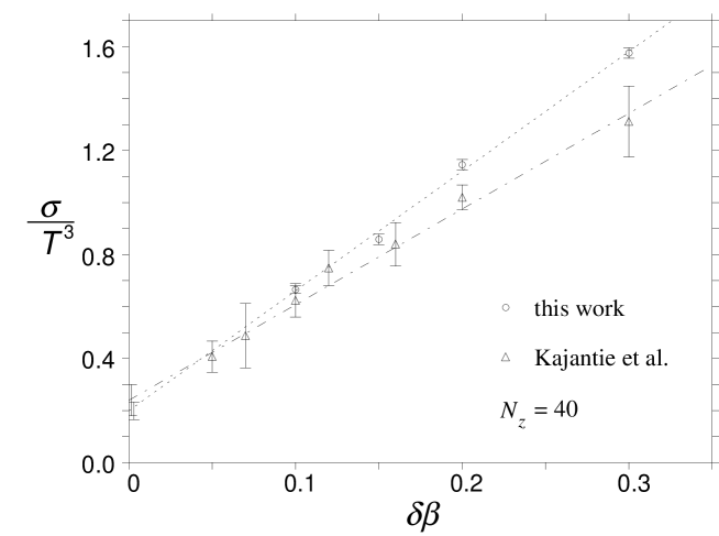
Figure 2: $\sigma$ with the operator method as a function of $\delta\beta$ on an $8^{2}\times 40\times 2$ lattice. Open circles are for our results and triangles are for those of Kajantie et al.[3].

In Fig. 2 we compare our data on an $8^{2}\times 40\times 2$ lattice with those of Kajantie et al.[3] on the same size of lattice. We observe that our results at a finite $\delta\beta$ are larger than their values. The discrepancy is ascribed to the difference in the assignment of the coupling constant for creating the interface as was discussed in Sect. 2. The discrepancy diminishes for a smaller $\delta\beta$, and our extrapolated value $\sigma/T_{c}^{3}=0.199(34)$ is consistent with the result 0.24(6) by Kajantie et al.

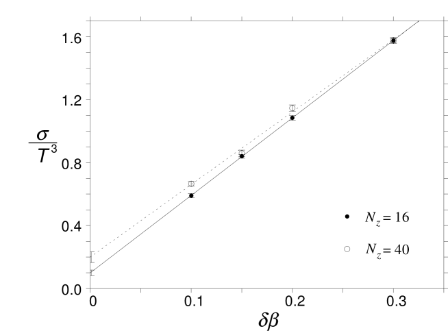
Figure 3: $\sigma$ with the operator method as a function of $\delta\beta$. Small filled circles are the results for the $8^{2}\times 16\times 2$ lattice, and open circles for the $8^{2}\times 40\times 2$ lattice.

Our results on an $8^{2}\times 16\times 2$ lattice is smaller than those on an $8^{2}\times 40\times 2$ lattice as shown in Fig 3. The difference increases with decreasing $\delta\beta$, and a linear extrapolation toward $\delta\beta=0$ results in a factor two difference in the values of $\sigma/T_{c}^{3}$ for the two lattice sizes (see the last column of Table 4).

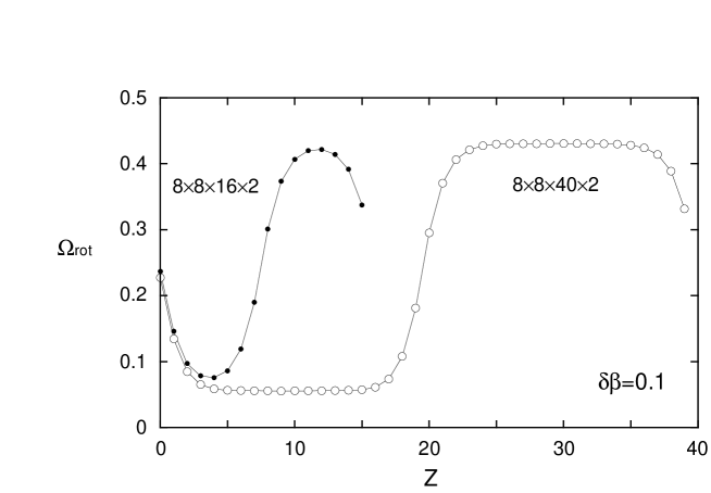
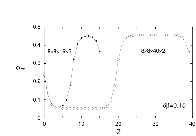
Figure 4: Real part of the rotated Polyakov loop as a function of $z$ on the $8^{2}\times 16\times 2$ and $8^{2}\times 40\times 2$ lattices. The Polyakov loop is rotated by a $Z(3)$ phase factor so that the argument is in (-$\pi/3$,$\pi/3$]. Errors are much smaller than the symbols. (a) for $\delta\beta=0.1$ and (b) $\delta\beta=0.15$.

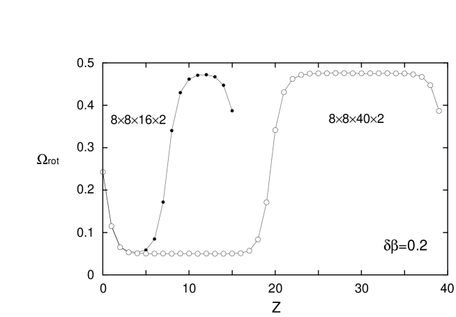
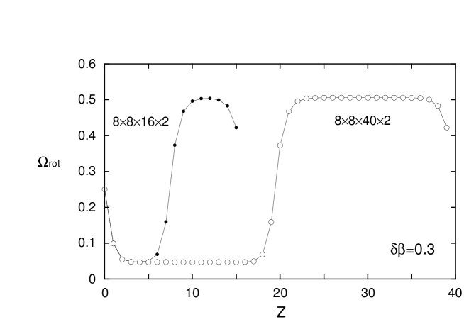
Figure 4: (Continued) (c) $\delta\beta=0.2$ and (d) $\delta\beta=0.3$.

To understand the origin of this size dependence, we study the spatial thickness of the interface. In Fig. 4 we show the $z$-dependence of the Polyakov loop rotated to the nearest $Z(3)$ axis $\Omega_{\rm rot}(N_{z})$ for various $\delta\beta$. For the larger lattice with $N_{z}=40$ we observe a clear plateau away from the the interface centers at $z=0$ and $N_{z}/2$ for all values of $\delta\beta$. In contrast, a plateau is barely visible for the $N_{z}=16$ lattice even for $\delta\beta=0.3$. Furthermore, for $\delta\beta\stackrel{{\scriptstyle<}}{{\scriptstyle\sim}}0.15$, $\Omega_{\rm rot}(16)$ deviates not only from the asymptotic values of $\Omega_{\rm rot}(40)$ but also from $\Omega_{\rm rot}(40)$ at the same distance from the interface center even at the middle points $z=4$ and 12 between interfaces. These observations suggest that the half width of the interface region is larger than 4 and consequently the two interfaces are affecting each other on the $N_{z}=16$ lattice.

Similar behavior is also found for the $z$-dependence of the interface free energy, albeit with larger errors. In Fig. 5 we plot the quantity $\tilde{\sigma}(d)$ obtained by restricting the summation in (2) for the interface tension to the two regions within a distance $d$ from the interface centers at $z=0$ and $N_{z}/2$. For $\delta\beta=0.1$, we find that $\tilde{\sigma}(d)$ on the $N_{z}=40$ lattice saturates only after $d=5-6$, and that $\tilde{\sigma}(d)$ for $N_{z}=16$ is clearly not saturated within the distance $d\leq 4$ available on this lattice. Furthermore the value of $\tilde{\sigma}(d)$ for $N_{z}=16$ is smaller than that for $N_{z}=40$ at $d\sim 2$ – 4. From these observations, we conclude that $N_{z}=16$ is not large enough to have two free interfaces within the spatial extent of the lattice. We also note that the smaller interface free energy observed for $N_{z}=16$ corresponds to an attractive interaction between opposite interfaces.

Another problem with the results in Table 4 is that they were obtained employing one-loop perturbative results for the response functions $c_{t}$ and $c_{s}$ and the lattice bare coupling $\beta$ in (2). This represents a questionable point since the critical coupling constant on an $N_{t}=2$ lattice is large. In order to examine how non-perturbative effects possibly affect the values of response functions[16], we recall that the combination $c_{t}+c_{s}$ is proportional to the scaling beta function: $c_{t}+c_{s}=-{a\over 2}({{\partial\beta}\over{\partial a}}).$ A non-perturbative estimate of this quantity is available from Monte-Carlo renormalization group studies[17], which shows a large deviation of the $\beta$ function from the perturbative result for $\beta\stackrel{{\scriptstyle<}}{{\scriptstyle\sim}}6$. The coefficients $c_{t}$ and $c_{s}$ also appear in other thermodynamic quantities, the energy density $\epsilon$ and the pressure $p$[18]. In fact the combination $\epsilon-3p$ is proportional to $c_{t}+c_{s}$, while $\epsilon+p$ depends both on $c_{t}+c_{s}$ and $c_{t}-c_{s}$. The problem with perturbative estimates of response functions manifests here not only in a scaling violation of $\epsilon$ and $p$ but also in a non-vanishing pressure gap at the first order deconfining transition [19]. We can therefore determine $c_{t}-c_{s}$ at $\beta_{c}$ by combining the results for the beta function from Monte-Carlo renormalization group studies with the requirement of a vanishing pressure gap.

Applying this procedure to the data obtained on $24^{2}\times 36\times 4$ and $36^{2}\times 48\times 6$ lattices [14], we find that

$$c_{t}-c_{s} = -0.52(12)\qquad\beta=5.6925$$ (9)

$$= -0.37(16)\qquad\beta=5.8936$$

($c_{t}=-0.24(6)$ and $-0.16(8)$ and $c_{s}=0.28(6)$ and $0.21(8)$ for the two values of $\beta$, respectively.) These values should be compared with the perturbative value,

$$c_{t}-c_{s}=-0.3336+O(\beta^{-1}).$$ (10)

The non-perturbative estimates (9) imply that the value for the interface tension will be reduced by a factor of 0.88(8) for $N_{t}=4$ and 0.98(10) for$N_{t}=6$ from that with the perturbative value using (10). This leads us to expect a reduction of the interface tension by perhaps an even larger magnitude for $N_{t}=2$ if non-perturbatively determined response functions are employed. A quantitative estimation of the magnitude of reduction, however, requires the value of the effective beta function at the critical coupling $\beta_{c}=5.09$ which is not available at present.

We should note that the discussion and the conclusion from Fig. 5 concerning finite-size effects are not affected by the correction to $c_{t}$ and $c_{s}$ because the main effect of it is a shift of the overall coefficient of $\sigma$.

3.2 Integral method

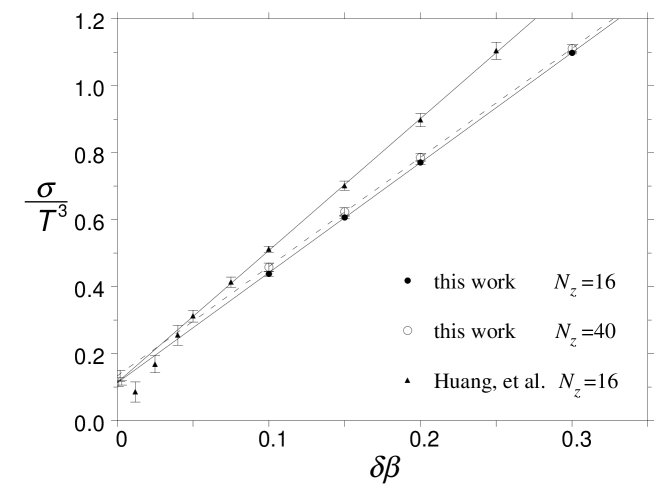
Figure 6: $\sigma$ with the integral method as a function of $\delta\beta$. Filled circles are the results of the $8^{2}\times 16\times 2$ lattice, and open circles those of the $8^{2}\times 40\times 2$ lattice. Triangles are the results of Huang, et al. [5] for $N_{z}=16$.

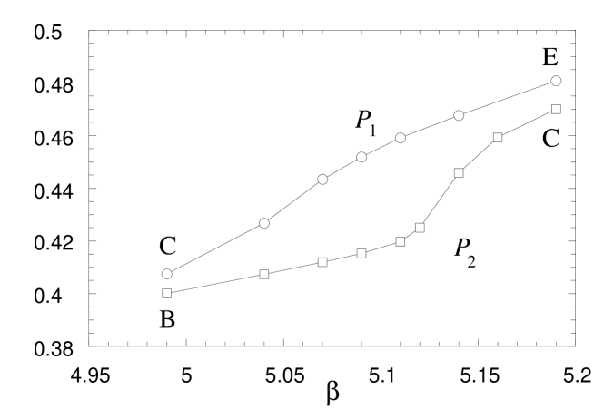
Figure 7: Plaquette expectation value in domain 1 along the path CE of Fig. 1 and that in domain 2 along BC on the $8^{2}\times 16\times 2$ lattice. Estimated errors are much smaller than the size of symbols.

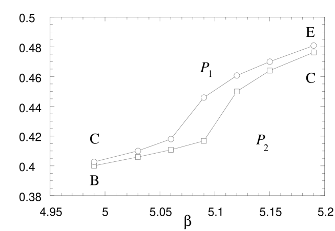
Figure 8: The same as Fig. 7 obtained on the $8^{2}\times 40\times 2$ lattice.

In Table 5 we summarize our results for $\sigma/T_{c}^{3}$ for the integral method. As is seen in Fig. 6 the data lie on a straight line with respect to $\delta\beta$. The results of a linear extrapolation are also given in Table 5. In Figs. 7 and 8 we plot the plaquette expectation values in the two halves of lattice as a function of $\beta$ along the integration path for the case of $\delta\beta=0.1$. The area surrounded by the two lines gives an estimate of $\sigma$.

As in the case of the operator method we find that our values for $N_{z}=16$ has a different slope from the corresponding results of Huang et al.[5] at finite $\delta\beta$ (compare filled circles and triangles in Fig. 6), while the value extrapolated to $\delta\beta=0$ is perfectly consistent, namely we find $\sigma/T_{c}^{3}=0.113(6)$ as compared to $\sigma/T_{c}^{3}=0.115(13)$ in ref. [5].

The results on an $8^{2}\times 40\times 2$ lattice are larger by about 5-10% from those on an $8^{2}\times 16\times 2$. The difference increases to 20% after extrapolation to $\delta\beta=0$, which, however, is much smaller compared to the case of the operator method where a factor two discrepancy is observed. We also note that the size effect is not sensitive to the value of $\delta\beta$ (Fig. 6), in contrast to the case of the operator method discussed in the previous subsection.

The origin of this difference of lattice size dependence may be understood in the following way. We expect the size effect on the interface to increase when both $\beta_{1}$ and $\beta_{2}$ become close to $\beta_{c}$ while keeping $\beta_{1}<\beta_{c}<\beta_{2}$. With our choice of the integration path as shown in Fig. 1, the size effect is therefore largest at the point C, diminishing toward the points D, B and E. Near the points B and E and along the paths BA and EF we expect size effects to be small because of the absence of the interface. We now recall that the interface tension in the integral method is obtained from the integrals along the paths ABCD and DCEF, while that with the operator method is taken at a point along the path DC. We then expect the magnitude of size effects to be smaller in the integral method since the large size effect near the point C, directly affecting results for the operator method, is diluted by contribution from other parts of the paths suffering less from the effects. Furthermore the fact that the paths BC and CE are common to all of our choices of $\delta\beta$ explains a similar magnitude of size effects seen in Fig. 6.

Comparing the results for $N_{z}=40$, we find that the value of $\sigma/T_{c}^{3}$ obtained by the operator method (with the perturbative coefficients) is larger than that of the integral method by a factor of about 1.5. We ascribe this discrepancy to the presence of non-perturbative corrections to the response functions based on the consideration discussed in the previous subsection.

We also note that our result $\sigma/T_{c}^{3}=0.134(16)$ with the integral method is consistent with a value $\sigma/T_{c}^{3}=0.139(4)$ from a determination with a transfer matrix method on $4^{4}\times 64\times 2$ – $8^{2}\times 128\times 2$ lattices[6], while a determination with a histogram method on $8^{2}\times 30\times 2$ – $14^{2}\times 42\times 2$ lattices [9] gives a slightly smaller value 0.092(4).

4 Results for $N_{t}=4$

Our comparative analysis of the operator and integral methods for $N_{t}=2$ lattices shows that the integral method suffers much less from various systematic errors. We therefore adopt the integral method for our study on an $N_{t}=4$ lattice.

A difficulty in an extraction of the interface tension for $N_{t}=4$ is the smallness of the value of $\sigma a^{3}$. In fact assuming scaling the result $\sigma/T_{c}^{3}\sim 0.1$ for $N_{t}=2$ leads to $\sigma a^{3}\sim 0.0015$ for $N_{t}=4$. The actual value appears even smaller; the value $\sigma/T_{c}^{3}=0.027(4)$ [12] obtained with the integral method using an external field coupled to the Polyakov loop translates to $\sigma a^{3}=0.00042(6)$. Thus very accurate results of plaquette expectation values for $\delta\beta$ much smaller than those employed for the case of $N_{t}=2$ will be needed. Furthermore it is known that a spatial size of at least 4–5 times larger than the temporal size is needed for clear first-order signals on an $N_{t}=4$ lattice[20, 14]. This requirement was not met in the first attempt [5] toward an interface tension measurement on an $N_{t}=4$ lattice, which failed to find a finite value of $\sigma$ employing $8^{2}\times 16\times 4$ and $12^{2}\times 24\times 4$ lattices. Based on those considerations we chose to work on an $18^{2}\times 48\times 4$ lattice and carried out simulations for $\delta\beta=0.02$ – 0.06.

As discussed in the previous section, a large $N_{z}$ is required to remove the effect of interface thickness. In Fig. 9 we plot $\Omega_{\rm rot}$ for $\delta\beta=0.02$ and 0.04 as a function of $z$. We observe a plateau for both cases, albeit somewhat limited in range for $\delta\beta=0.02$. From our experience with the $N_{t}=2$ lattices we consider that the effect of interface thickness is sufficiently suppressed for $\delta\beta\stackrel{{\scriptstyle>}}{{\scriptstyle\sim}}0.02$

Our result for $\sigma$ is summarized in Table 6 and plotted in Fig. 10. Taking the three points with $\delta\beta\leq 0.04$ and extrapolating linearly toward $\delta\beta=0$ we find $\sigma/T_{c}^{3}=0.0171(113)$. The central value is smaller than the previous estimate $\sigma/T_{c}^{3}=0.027(4)$ obtained on a $16^{2}\times 32\times 4$ lattice [12]. We note that a recent study with the histogram method using the data of [14] on lattices $12^{2}\times 24\times 4$ and $24^{2}\times 36\times 4$ also gives a larger value 0.0292(22) [21]. The error in our result, however, is too large to see if there is a real discrepancy.

5 Conclusions

We have studied the confinement-deconfinement interface tension in the pure $SU(3)$ gauge theory on an $8^{2}\times N_{z}\times 2$ lattice with $N_{z}=16$ and 40 by applying the operator and integral methods. Our results confirm the values reported previously when compared at the same parameters. Our study of the $N_{z}$ dependence shows, however, that the thickness of the interface causes misleadingly smaller values for the interface tension $\sigma$ when estimated on a lattice of a small length such as $N_{z}=16$. This effect is severer for the operator method, which explains part of the discrepancy in the interface tension obtained with the two methods. We made some quantitative estimates on non-perturbative corrections to the responce function $c_{t}-c_{s}$ needed in the operator method, and argued that incorporating them would remove the rest of the discrepancy. We conclude that the integral method yields more reliable values for the interface tension, suffering less from various systematic errors. Our result $\sigma/T_{c}^{3}=0.134(16)$ with the integral method on a large lattice is consistent with a determinations with a transfer matrix method[6].

We have also attempted a measurement of the interface tension on an $N_{t}=4$ lattice with the integral method. The result is smaller than those reported in the literature[12, 21]. It has quite a large error, however, in spite of the substantial statistics accumulated with 14 days of fully running QCDPAX. The problem originates from a rapid decrease of the discontinuity in plaquette averages with an increasing $N_{t}$. A judicious choice of observables having a larger jump across the deconfining transition as was done by Brower et al.[12] will be indispensable for a determination of the interface tension closer to the limit of continuum space-time.

		run parameters
$\beta_{1}$	$\beta_{2}$	tot. sw.	therm.	$P_{1}$		$P_{2}$		$P_{2}-P_{1}$
4.79		21000	1000	0.373370 (45)
4.89		21000	1000	0.386170 (37)
4.94		21000	1000	0.392992 (41)
4.99		30000	1000	0.400056 (46)
5.00		30000	1000	0.401590 (48)
5.04		30000	1000	0.407723 (55)
5.07		30000	1000	0.41261   (10)
5.09		198000	8000	0.4278     (15)
5.11		30000	1000	0.45551   (22)
5.14		30000	1000	0.46652   (12)
5.19		30000	1000	0.480807 (95)
5.24		30000	1000	0.492618 (75)
5.29		21000	1000	0.503312 (75)
5.39		24000	4000	0.521825 (68)
4.99	5.19	200000	10000	0.407549  (	86)	0.470238  (	92)	0.062689  (	79)
4.94	5.24	200000	10000	0.399601  (	45)	0.482138  (	60)	0.082537  (	52)
4.89	5.29	125000	10000	0.392557  (	42)	0.492648  (	59)	0.100091  (	56)
4.79	5.39	200000	10000	0.379668  (	27)	0.511044  (	35)	0.131376  (	37)
4.99	5.04	30000	3000	0.400363  (	64)	0.407368  (	60)
4.99	5.07	60000	3000	0.400476  (	50)	0.411974  (	58)
4.99	5.09	60000	3000	0.400610  (	45)	0.415267  (	67)
4.99	5.11	60000	3000	0.400846  (	61)	0.41970  (	31)
4.99	5.12	60000	3000	0.40124  (	10)	0.42504  (	77)
4.99	5.14	60000	3000	0.40338  (	15)	0.4459  (	10)
4.99	5.16	60000	3000	0.40539  (	14)	0.45930  (	35)
5.04	5.19	60000	3000	0.42676  (	32)	0.47455  (	15)
5.07	5.19	60000	3000	0.44340  (	31)	0.47709  (	11)
5.09	5.19	60000	3000	0.4519  (	16)	0.477845  (	97)
5.11	5.19	60000	3000	0.45917  (	12)	0.478778  (	82)
5.14	5.19	30000	3000	0.46769  (	14)	0.47928  (	11)

Table 1: Run parameters and plaquette expectation values in each domain on the $8^{2}\times 16\times 2$ lattice. These simulation points are plotted in Fig. 1.

		run parameters
$\beta_{1}$	$\beta_{2}$	tot. sw.	therm.	$P_{1}$		$P_{2}$		$P_{2}-P_{1}$
4.79		22000	4000	0.373399 (23)
4.89		20000	2000	0.386199 (28)
4.94		20000	2000	0.392953 (31)
4.99		20000	2000	0.400122 (35)
5.03		20000	2000	0.406027 (45)
5.06		20000	2000	0.410851 (48)
5.09		100000	10000	0.41918   (99)
5.0937		530000	30000	0.4306     (18)
5.12		20000	2000	0.45931   (15)
5.15		20000	2000	0.46963   (10)
5.19		20000	2000	0.480845 (80)
5.24		20000	2000	0.492589 (62)
5.29		20000	2000	0.503317 (47)
5.39		22000	4000	0.521852 (41)
4.99	5.19	400000	20000	0.402641  (	20)	0.476307  (	29)	0.073666  (	26)
4.94	5.24	200000	10000	0.395490  (	19)	0.488416  (	29)	0.092926  (	30)
4.89	5.29	200000	10000	0.388714  (	15)	0.499055  (	25)	0.110341  (	26)
4.79	5.39	200000	10000	0.375886  (	13)	0.517555  (	20)	0.141669  (	23)
4.99	5.03	26000	5000	0.400123  (	73)	0.405956  (	66)
4.99	5.06	24000	3000	0.400268  (	43)	0.410796  (	72)
4.99	5.09	52000	4000	0.400280  (	37)	0.41675  (	39)
4.99	5.12	24000	3000	0.400989  (	59)	0.44999  (	35)
4.99	5.15	24000	3000	0.401837  (	58)	0.46402  (	17)
5.03	5.19	24000	3000	0.41004  (	12)	0.47712  (	11)
5.06	5.19	24000	3000	0.41804  (	34)	0.47823  (	19)
5.09	5.19	74000	6000	0.44597  (	67)	0.479589  (	71)
5.12	5.19	24000	3000	0.46070  (	15)	0.480154  (	79)
5.15	5.19	24000	3000	0.47006  (	14)	0.48020  (	10)

Table 2: The same as Table 1 for the $8^{2}\times 40\times 2$ lattice.

		run parameters						$P_{2}-P_{1}$
$\beta_{1}$	$\beta_{2}$	tot. sw.	therm.	$P_{1}$		$P_{2}$		$\times 10^{2}$
5.6324		12000	2000	0.533130 (38)
5.6524		12000	2000	0.538238 (46)
5.6624		12000	2000	0.540762 (45)
5.6724		20000	2000	0.543113 (32)
5.6804		20000	2000	0.545051 (44)
5.6870		20000	2000	0.54692   (20)
5.6924		80000	5000	0.54873   (30)
5.6978		20000	2000	0.552987 (53)
5.7044		20000	2000	0.554618 (51)
5.7124		20000	2000	0.556508 (34)
5.7224		12000	2000	0.558488 (36)
5.7324		12000	2000	0.560475 (32)
5.7524		12000	2000	0.563854 (25)
5.6724	5.7124	32000	4000	0.544131  (	67)	0.555520  (	66)	1.1390  (	87)
5.6624	5.7224	32000	4000	0.541635  (	75)	0.557411  (	89)	1.5776  (	57)
5.6524	5.7324	32000	4000	0.539321  (	44)	0.559379  (	35)	2.0058  (	45)
5.6324	5.7524	32000	4000	0.534442  (	33)	0.562714  (	25)	2.8272  (	39)
5.6124	5.7724	32000	4000	0.529389  (	40)	0.565739  (	21)	3.6350  (	47)
5.6724	5.682	60000	2000	0.543233  (	24)	0.545364  (	30)
5.6724	5.688	60000	2000	0.543296  (	33)	0.546843  (	63)
5.6724	5.694	100000	4000	0.543410  (	52)	0.54871  (	10)
5.6724	5.700	120000	4000	0.543513  (	50)	0.55092  (	21)
5.6724	5.706	60000	2000	0.543827  (	41)	0.553736  (	77)
5.678	5.7124	60000	2000	0.545623  (	80)	0.555678  (	50)
5.684	5.7124	100000	4000	0.54831  (	11)	0.556022  (	29)
5.690	5.7124	88000	4000	0.550893  (	83)	0.556265  (	26)
5.696	5.7124	40000	2000	0.552771  (	52)	0.556342  (	33)
5.702	5.7124	40000	2000	0.554249  (	45)	0.556372  (	37)

Table 3: The same as Table 1 for the $18^{2}\times 48\times 4$ lattice. The last run in the second group was not used in the integral method.

	$\delta\beta$
$N_{z}$	0.3	0.2	0.15	0.1	$\sigma/T_{c}^{3}$	$\chi^{2}/dof$
16	1.575 (12)	1.084 (16)	0.840 (13)	0.590 (14)	0.100 (18)	0.03
40	1.575 (20)	1.146 (20)	0.859 (20)	0.665 (15)	0.199 (34)	2.15

Table 4: $\sigma(\delta\beta)/T_{c}^{3}$ for $N_{t}=2$ at finite $\delta\beta$ determined with the operator method. The last two columns are the results of a linear extrapolation to $\delta\beta=0$ and its $\chi^{2}$ per degree of freedom.

	$\delta\beta$
$N_{z}$	0.3	0.2	0.15	0.1	$\sigma/T_{c}^{3}$	$\chi^{2}/dof$
16	1.098 (4)	0.771 (5)	0.607 (4)	0.438 (7)	0.113 (6)	0.17
40	1.111 (11)	0.786 (13)	0.624 (12)	0.458 (12)	0.134 (16)	0.01

Table 5: $\sigma(\delta\beta)/T_{c}^{3}$ for $N_{t}=2$ determined with the integral method. The last two columns are the results of a linear extrapolation to $\delta\beta=0$.

$\delta\beta$
0.06	0.04	0.03	0.02	$\sigma/T_{c}^{3}$	$\chi^{2}/dof$
0.6031(122)	0.3897(67)	0.2945(68)	0.2034(45)	0.0171(113)	0.06

Table 6: $\sigma(\delta\beta)/T_{c}^{3}$ for $N_{t}=4$ determined with the integral method. The last two columns are the results of a linear extrapolation to $\delta\beta=0$ using $\delta\beta=0.02$ – 0.04.

Figure 1: The Monte Carlo simulation points for $N_{t}=2$ in the space of $(\beta_{+},\beta_{-})$. Small filled circles are the simulation points for an $8^{2}\times 16\times 2$ lattice, and open circles for an $8^{2}\times 40\times 2$ lattice. The symbol “+” corresponds to the phase transition point $(\beta_{c},\beta_{c})$.

Figure 5: $\tilde{\sigma}(d)$ defined as $\sigma/T_{c}^{3}$ with the operator method with restricting the summation in (2) to the regions within the distance $d$ from $z=0$ and $N_{z}/2$. ($\tilde{\sigma}(N_{z}/4)\equiv\sigma/T_{c}^{3}$ given in Table 4.)

Figure 9: Real part of the rotated Polyakov loop as a function of $z$ on the $18^{2}\times 48\times 4$ lattice for $\delta\beta=0.02$ and 0.04.

Figure 10: $\sigma$ with the integral method as a function of $\delta\beta$ on the $18^{2}\times 48\times 4$ lattice. The line is the result of linear fit to the data at $\delta\beta=0.02$ – 0.04.

References

- [1] For a review of evidence, see, A. Ukawa, in Proceedings of Lattice’89, Nucl. Phys. B(Proc. Suppl.)
- [2] K. Kajantie and L. Kärkkäinen, Phys. Lett. B214 (1988) 595.
- [3] K. Kajantie, L. Kärkkäinen and K. Rummukainen, Nucl. Phys. B 333 (1990) 100
- [4] J. Potvin and C. Rebbi, Phys. Rev. Lett. 62 (1989) 3062.
- [5] S. Huang, J. Potvin, C. Rebbi and S. Sanielevici, Phys. Rev. D 42 (1990) 2864; errata 43 (1991) 2056.
- [6] B. Grossmann, M.L. Laursen, T. Trappenberg and U.-J. Wiese, Nucl. Phys. B396 (1993) 584.
- [7] W. Janke, B.A. Berg and M. Katoot, Nucl. Phys. B382 (1992) 649;
- [8] B. Grossmann, M.L. Laursen, T. Trappenberg and U.-J. Wiese, Phys. Lett. B293 (1992) 175.
- [9] B. Grossmann, M.L. Laursen, Jülich preprint HLRZ-93-7, revised, to appear in Nucl. Phys. B.
- [10] K. Binder, Z. Phys. B43 (1981) 119; Phys. Rev. A25 (1982) 1699.
- [11] F. Karsch, Nucl. Phys. B205[FS5] (1982) 285.
- [12] R. Brower, S. Huang, J. Potvin and C. Rebbi, Phys. Rev. D 46 (1992) 2703.
- [13] I.R. McDonald and K. Singer, Discuss. Faraday Soc. 43 (1967) 40; A.M. Ferrenberg and R. Swendsen, Phys. Rev. Lett. 61 (1988) 2058; 63 (1989) 1195.
- [14] Y. Iwasaki, K. Kanaya, T. Yoshié, T. Hoshino, T. Shirakawa, Y. Oyanagi, S. Ichii and T. Kawai, Phys. Rev. D 46 (1992) 4657.
- [15] Y. Iwasaki et al., Computer Physics Communications 49 (1988) 449; Y. Iwasaki et al., Nucl. Phys. B (Proc. Suppl.) 17 (1990) 259; T. Hoshino, PAX Computer, High-Speed Parallel Processing and Scientific computing (Addison-Wesley, New York, 1989).
- [16] For an early attempt for a non-perturbative study, see, G. Burger et al., Nucl. Phys. B304 (1988) 587.
- [17] A. Hasenfratz et al., Phys. Lett. B140 (1984) 76; K.C. Bowler et al., Nucl. Phys. B257[FS14] (1985) 155; A.D. Kennedy et al., Phys. Lett. B155 (1985) 414; R. Gupta et al., Phys. Lett. B211 (1988) 132; J. Hoek, Nucl. Phys. B339 (1990) 732.
- [18] J. Engels et al., Nucl. Phys. B205[FS5] (1982) 545.
- [19] J. Engels et al., Phys. Lett. B252 (1990) 625.
- [20] M. Fukugita, M. Okawa and A. Ukawa, Nucl. Phys. B337 (1990) 181.
- [21] Y. Iwasaki, K. Kanaya, L. Kärkkäinen, K. Rummukainen and T. Yoshié, preprint UTHEP-252 (1993).