hep-lat/9311062 DFTUZ 93/18 November 1993
Phase diagram of a lattice $SU(2)\times SU(2)$ scalar-fermion model using the Zaragoza fermions

Abstract

We present a calculation of the phase diagram of a $SU(2)\times SU(2)$ chiral Yukawa model with massless decoupled doublers, using a saddle point approach, both for small and large Yukawa coupling. Some preliminary MonteCarlo results are also shown.

1 INTRODUCTION

A lattice regularization of the Standard Model (SM) is necessary not only to establish the existence of chiral gauge theories outside perturbation theory, but also to understand various properties of the fermion mass generation by spontaneous symmetry breaking such as, for instance, the upper bounds on top and Higgs masses[1]. For this purpose it is sufficient to study the fermion-scalar sector of the SM which is essentially a Chiral Yukawa Model (CYM).

In this talk, we determine the phase structure of a $SU(2)\times SU(2)$ CYM, using Zaragoza fermions[2]. We decided to freeze the radial mode of the scalar field. This corresponds to the choice of an infinite bare quartic coupling. For a comparison with the phase structure of other related models see[1, 3].

2 LATTICE REGULARIZED CHIRAL YUKAWA MODEL

Consider $N_{d}$ $SU(2)$ fermion doublets $\psi$, and a $2\times 2$ $SU(2)$ matrix, $\phi$. The action can be cast into the form [2]

$$S(\psi,\phi)=S_{B}(\phi)+S_{F}(\psi)+S_{Y}(\widehat{\psi},\phi),$$ (1)

where

$$S_{B}(\phi)=-{\kappa\over 2}\sum_{x,\mu}Tr\left(\phi_{x+\hat{\mu}}^{\dagger}\phi_{x}+\phi_{x}^{\dagger}\phi_{x+\hat{\mu}}\right)$$ (2)

is the lattice action for a scalar with frozen radial modes. $S_{F}(\psi)$, the free fermionic action is

$$S_{F}(\psi)={1\over 2}\sum_{\psi,x,\mu}\left(\overline{\psi}_{x}\gamma_{\mu}\psi_{x+\hat{\mu}}-\overline{\psi}_{x+\hat{\mu}}\gamma_{\mu}\psi_{x}\right),$$ (3)

and the interaction term is

$$S_{Y}(\widehat{\psi},\phi)=y\sum_{\psi,x}\left(\widehat{\overline{\psi}}_{Lx}\phi_{x}\widehat{\psi}_{Rx}+\widehat{\overline{\psi}}_{Rx}\phi_{x}^{\dagger}\widehat{\psi}_{Lx}\right).$$ (4)

Our way of implementing the decoupling of doublers is based on the use of the $\widehat{\psi}$ fields. In momentum space,

$$\widehat{\psi}(k)=F(k)\psi(k),\quad F(k)=\prod_{\mu}\cos\left({k_{\mu}\over 2}\right).$$ (5)

In coordinate space this corresponds to an average of fields $\psi$ over an elementary hypercube

$$\widehat{\psi}_{x}={1\over 2^{4}}\sum_{b}\psi_{x+b},\quad b_{\mu}=0,1.$$ (6)

The model has a global chiral $SU(2)\times SU(2)$ symmetry

$$\psi_{L}(x)\to\Omega_{L}\psi_{L}(x),\qquad\psi_{R}(x)\to\Omega_{R}\psi_{R}(x),$$

$$\phi(x)\to\Omega_{L}\phi(x)\Omega_{R}^{\dagger},$$ (7)

where $\Omega_{R},\Omega_{L}\in SU(2)$. (A corresponding transformation acts on the barred fermions).

3 DECOUPLING OF DOUBLERS

The model has been constructed to show decoupling at tree level. The fermion-scalar vertex is given by

$$V(k,k^{\prime})=yF(k)F(k^{\prime}),$$ (8)

and the particular choice of $F(k)$ makes it vanish for every doubler fermion (any $k_{\mu}$ or $k_{\mu}^{\prime}=\pi$). It can also be shown that at any order in perturbation theory, the renormalized Green functions are the same as the continuum ones. The proof[2] is based on the Riesz power counting theorem. There are also ($2^{4}-1$) Golterman-Petcher like symmetries[2, 4] which can be used to argue that the doubler fermions also decouple in the nonperturbative regime, provided a sensible continuum limit exists.

An important characteristic of our decoupling method is that the $U$, $S$ and $\Delta\rho$ parameters (which describe the radiative corrections to the electroweak interaction observables coming from the Higgs sector) do not receive, at one loop level, contributions from the counterterms needed to recover gauge invariance[5]. This allows us, using only the scalar-fermion sector of the SM, to compute $\Delta\rho$ non-perturbatively. Prior to do this and the computation of upper bounds on top and Higgs masses a phase diagram is required.

4 MEAN FIELD CALCULATION OF THE PHASE DIAGRAM

We have performed an analytic calculation of the phase diagram, using mean field techniques, both for small and large values of the Yukawa coupling $y$.

There are two essential steps.

$\bullet$ First. With the aid of two auxiliary scalar fields, one performs the integration over the scalar field $\phi$.

$\bullet$$\bullet$ For small $y$, one expands $\exp\left\{-S_{Y}\right\}$ arround 1, up to four fermion terms before integrating out the scalar field.

$\bullet$$\bullet$ For large $y$, auxiliary fermions $\eta$ are used in order to change the coupling parameter to $1/y$. In particular, for one fermion doublet,

$$\exp\left\{-S_{Y}\right\}\propto\int\left[d\eta d\overline{\eta}\right]exp\left\{\overline{\eta}\widehat{\psi}+\widehat{\overline{\psi}}\eta\right\}$$

$${}\times\exp\left\{{1\over y}\overline{\eta}\left(\phi^{+}P_{R}+\phi P_{L}\right)\eta\right\}.$$ (9)

One can now perform an expansion of the exponential around 1, up to four fermion terms, then integrate out the scalar field. Finally one integrates over the auxiliary $\eta$.

$\bullet$ Second. After replacing the auxiliary fields with their saddle point solutions one is able to calculate (in both regimes) the fermion determinant and therefore the Free energy.

Figure 1: Mean field calculation of the phase diagram. The number of fermion doublets ($N_{d}$) is two.

The order parameters we have used to distinguish the phases are

$$\left\langle\phi\right\rangle=\left\langle{1\over V}\sum_{n}\phi_{n}\right\rangle$$ (10)

and

$$\left\langle\phi_{st}\right\rangle=\left\langle{1\over V}\sum_{n}\epsilon_{n}\phi_{n}\right\rangle,$$ (11)

where $\epsilon_{n}={(-1)}^{n_{1}+\dots+n_{4}}$.

There are four phases:

$\bullet$ FM: In this phase $\left\langle\phi\right\rangle\not=0$ and $\left\langle\phi_{st}\right\rangle=0$.

$\bullet$ PM: Here, $\left\langle\phi\right\rangle=\left\langle\phi_{st}\right\rangle=0$.

$\bullet$ AF: This phase is characterized by $\left\langle\phi\right\rangle=0$ and $\left\langle\phi_{st}\right\rangle\not=0$.

$\bullet$ FI: Both parameters are different from zero.

The mean field results are presented in figures 1 and 2, where the range of validity for both small and large $y$ expansions can be appreciated ($y<11$ and $y>6\times 10^{6}$ respectively). For small $y$ the expected FM–PM–AFM structure appears together with a quadruple point and a FI phase. For large $y$ only two phases appear, FM and FI, so that the shape of funnel is excluded for this model.

The phase transitions are second order within this mean field approach. In the same approach, we can understand why the PM-AF transition line is almost flat. This is a consequence of the decoupling. In fact, in the AF phase, the scalar field takes the form $\phi_{n}=v_{st}\epsilon_{n}$, thus it always carries momentum $\pi$. Due to momentum conservation, when this scalar interacts with two fermions, the latter must be either a physical fermion and a doubler or two different doublers. In either case, the interaction is supressed as doublers are decoupled. So, the critical hopping parameter $\kappa$ is not affected by the Yukawa coupling $y$. This behaviour is confirmed by the MonteCarlo results (Figure 2).

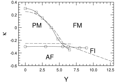
Figure 2: Phase diagram. Dashed lines correspond to the mean field calculation. Square and circle symbols are numerical results in a $4^{4}$ lattice. $N_{d}=2$.

5 MONTECARLO SIMULATION

The mean field calculation gives us a feeling for the phase diagram, but in order to have quantitative results we are doing a numerical simulation of this model with two doublets of fermions, using a Hybrid-MonteCarlo algorithm. Figure 2 shows some preliminary results for a $4^{4}$ lattice. They are in good agreement with the mean field computations. Current work includes a MonteCarlo simulation in a $8^{4}$ lattice. Using this larger lattice we expect first to get a clearer determination of the phase transition lines, second to calculate upper bounds on top and Higgs masses, and third to study non-perturbatively the $\Delta\rho$ parameter.

References

- [1] For a recent review see D.N. Petcher, Nucl. Phys. B (Proc. Suppl.) 30 (1993) 50.
-
[2]
J.L. Alonso, Ph. Boucaud, J.L. Cortés and E. Rivas,
Mod. Phys. Lett. A5 (1990) 275,
Phys. Rev. D44 (1991) 3258;
J.L. Alonso, Ph. Boucaud, J.L. Cortés, F. Lesmes and E. Rivas, Nucl. Phys. B (Proc. Suppl.) 29B,C (1992) 171. -
[3]
W. Bock, A.K. De, K. Jansen, J. Jersak, T. Neuhaus and J.
Smit,
Nucl. Phys. B 344, (1990) 207;
C. Frick, T. Trappenberg, L. Lin, G. Münster, M. Plagge, I. Montvay and H. Wittig, prepint DESY 92-11;
W. Bock, C. Frick, J. Smit and J.C. Vink, Nucl. Phys. B 400 (1993) 309;
I-H. Lee, J. Shigemitsu and R.E. Shrock, Nucl. Phys. B 330 (1990) 225;
S. Zenkin, KYUSHU-HET-8, September 1993. - [4] M.F.L. Golterman and D.N. Petcher, Phys. Lett. B225 (1989) 159.
- [5] J.L. Alonso, Ph. Boucaud, J.L. Cortés, F. Lesmes and E. Rivas, Nucl. Phys. B 407 (1993) 373.