$\alpha_{s}$ from the Lattice Potential

Abstract

We present an extensive study on the direct determination of the running coupling $\alpha_{s}$ from the static quark antiquark force at short distances, in quenched QCD. We find from our high statistics potential analysis that $\alpha_{q\bar{q}}$ exhibits two-loop asymptotic behaviour for momenta as low as $.5$ GeV. As a result, we determine the zero flavour $\Lambda$-parameter to be $\Lambda^{(0)}_{\overline{M\!S}}=.630(38)\sqrt{\sigma}=293(18)^{+25}_{-63}$ MeV. A rough estimate of full QCD effects leads to the five flavour value $\alpha_{\overline{M\!S}}(m_{Z})=.102^{+6}_{-11}$. A comparison with other lattice results is made.

1 INTRODUCTION

Considerable progress has been achieved over the past three years in the determination of the running coupling from SU(3) gauge theory, i.e. quenched QCD on the lattice. Just like in real experiment, this is not an easy task, since we are dealing with logarithmic effects. Moreover, asymptotic scaling is substantially violated in the $\beta$-window presently accessible to lattice simulations. This is to say that the perturbative two-loop-formula does not yet relate the lattice spacing $a$ to the bare coupling, $g_{0}^{2}=6/\beta$, in terms of a constant lattice scale $\Lambda_{L}$:

$$a\Lambda_{L}=\exp\left(-\frac{1}{2b_{0}g_{0}^{2}}\right)(b_{0}g_{0}^{2})^{-\frac{b_{1}}{2b_{0}^{2}}}\quad,$$ (1)

with

$$b_{0}=\frac{11}{16\pi^{2}}\quad,\quad b_{1}=\frac{102}{\left(16\pi^{2}\right)^{2}}\quad.$$ (2)

Therefore this perturbative relation in the bare lattice coupling scheme is not well suited for a determination of $\alpha_{s}$. This scheme is also too far off the continuum $\overline{M\!S}$-scheme to rely on the perturbative recoupling [1]

$$\alpha_{\overline{M\!S}}=\alpha_{L}+5.88\alpha^{2}_{L}+{\cal O}(\alpha^{3}_{L}),\quad\alpha_{L}=g_{0}^{2}/4\pi$$ (3)

at accessible lattice spacings.

Three major directions have been followed in the past to tackle the problem: (a) abandon the bare lattice coupling for the sake of “improved” coupling schemes on the lattice, which are better suited to renormalized perturbative expansions of short distance operators [2]; (b) determine $\alpha_{q\bar{q}}$ directly from the static $q\bar{q}$-force, on sufficiently large and fine lattices [3, 4]; (c) contrive a scheme with a volume dependent coupling $g(L)$. This novel access to the problem, put forward in Ref. [5], is intriguing as it lends itself to the application of finite-size matching techniques.

Figure 1: Comparison between the oscillation of the potential data (at $\beta=6.4$) around $V_{cont}$ and the expectation of Eq. (8).

Method (c) has been covered during last year’s conference with application to the SU(2) case [6]. The outcome for SU(3) gauge theory is presented in WOLFF’s talk [7], while the status of method (a) has been reviewed in the contribution of EL-KHADRA to this session [8].

We will focus here on the direct determination of $\alpha_{q\bar{q}}$ from the short distance force and report on the status of the analysis of high precision potential data in SU(3) gauge theory. In view of the quality of today’s data, the analysis method [3, 9] is devised to extract $\alpha_{q\bar{q}}$ locally at short distances rather than deriving it from a global ansatz to the force – with short and long distance boundary conditions – as proposed in Ref. [10].

We perform the “classical” Creutz experiment [11] and extract the potential from the local masses

$$V(\vec{R})=\ln\frac{W(R,T)}{W(R,T+1)}\quad,\quad T\,\,\,\mbox{large}\quad,$$ (4)

using improved techniques for suppression of excited state contributions in order to attain an early onset of the asymptotic plateau in $T$, as explained in Refs. [12, 4].

$\beta=$	5.5	5.6	5.7	5.8	5.9
$V=16^{4}$	400	200	200	400	220
$\beta=$	6.0	6.2	6.4	6.8
$V=32^{4}$	185	200	252	110

Table 1: The number of independent configurations produced and analysed on $16^{4}$ and $32^{4}$ lattices.

On more than 2000 independent configurations of $32^{4}$ and $16^{4}$ lattices (Tab. 1), measurements of on- and off-axis potentials have been carried out for 72 and 36 different $q\bar{q}$ separations $\vec{R}$, respectively, with resolutions ranging from $.03$ to $.25$ fm. UKQCD has another set of 50 $36^{4}$ configurations at $\beta=6.5$ with mostly on-axis potentials [13] measured.

Figure 2: The sensitivity of the on-axis force at $\beta=6.4$ on the parametrization of the potential.

The interquark force $F$ is expected to behave perturbatively at sufficiently short distances:

$$F(R)=-\frac{4}{3}\alpha_{q\bar{q}}(R)/R^{2}\quad.$$ (5)

Perturbation theory relates the $q\bar{q}$- and the $\overline{M\!S}$- schemes by means of a very small first-order coefficient [14]:

$$\alpha_{\overline{M\!S}}=\alpha_{q\bar{q}}-.086\alpha^{2}_{q\bar{q}}+{\cal O}(\alpha^{3}_{q\bar{q}})\quad.$$ (6)

This connection lets the $q\bar{q}$-scheme appear as a very promising candidate for a “perfect” lattice renormalization scheme [2].

2 UNFOLDING LATTICE ARTIFACTS

At present, an $\alpha_{s}$-analysis of the potential must rely on lattice data in the $R$-region from 2 to 7. This necessitates a careful treatment of lattice artifacts.

One expects [15] the continuum and lattice potentials to be related by a correction term

$$V(\vec{R})=V_{cont}(R)-\delta V(\vec{R})\quad,$$ (7)

which should be proportional to the difference between the lattice and continuum propagators:

$$\delta V({\vec{R}})=\gamma\left(4\pi G_{L}({\vec{R}})-1/R\right)\quad.$$ (8)

As one can see from Fig. 1 (circles), this correction exhibits significant oscillations around zero for $R\leq 4$, with maximal deflection occurring for the on-axis lattice potentials. For the determination of the parameter $\gamma$ in Eq. (8), we make use of two parametrizations of the continuum potential. We follow MICHAEL [3] and choose as the first form

$$V_{cont}(R)=V_{0}+KR-e/R+f/R^{2}\quad,$$ (9)

while the second is the Cornell potential from Eq. 14 ($f=0$). We demonstrate in Fig. 1, that this simple ansatz works surprisingly well: with the best fit value for $\gamma/e=l\approx.6$, which incidentally comes out independently of $\beta$ and $f$, the lattice potential data are seen to bounce around the interpolating curve in very much the same way as described by Eq. (8).

We emphasize again, that at this stage we are merely concerned with unfolding the lattice artifacts, and we better make sure that the unfolding procedure is sufficiently robust in the sense, that the resulting “continuum” force, $F$, is not an artifact of the underlying interpolative ansatz Eq. (9).

To that end, let us first define the force by discrete differentiation according to

$$F(\bar{R})=\\ \frac{V(\vec{R}_{1})-V(\vec{R}_{2})}{\Delta},\quad\Delta=R_{2}-R_{1}.$$ (10)

This definition carries an error ${\cal O}\left((\Delta/\bar{R})^{2}\right)$.

In order to reduce this discretization error, $\bar{R}$ should be properly placed within the interval $(R_{1},R_{2})$. We have exploited the parametrization, Eqs. (7,8,9), to compute this tangential point and estimate its error from the uncertainties of the fit parameters $l=\gamma/e$ and $f/e$. We assumed systematic errors of $20\%$ and $100\%$ on these parameters, respectively. The discretization effects, estimated in this manner, clearly dominate the errors at small $R$. For the subsequent analysis, we have chosen $1\leq\mid R_{2}-R_{1}\mid\leq 2$.

The parametrization dependence of $F$ is displayed in Fig. 2. The circles therein refer to Eq. (9) and squares to the Cornell form (Eq. (14)) of the potential. They differ by much less than the systematic errors we state. Note that, for the purpose of this figure, the (horizontal) shift in the tangent point $R$ has been converted into a (vertical) shift in $F$.

Figure 3: The plateau in $\Lambda_{R}(R)$ at $\beta=6.4$. The inner (outer) part of the errorbars refers to the statistical (systematic) uncertainties.

3 TWO-LOOP ANALYSIS

Given $F$, we base our $\alpha_{q\bar{q}}$-analysis on the two-loop prediction

$$F(R)=\\ \frac{1}{6\pi b_{0}}\frac{1}{R^{2}}\left(t-\frac{b_{1}}{2b_{0}^{2}}\ln(-2t))\right)^{-1}$$ (11)

with $t=\ln(\Lambda_{R}R)$. In this part of the analysis, we exclude those pieces of data on the force $F$ that involve $V(R=1)$, since the unfolding of lattice artifacts is not successful on this point, according to Fig. 1.

Figure 4: Scaling plot of the reconstructed continuum force. The perturbative region is zoomed in the inset. Full curve with errorband corresponds to the two-loop formula, with $\Lambda_{R}$ from Eq. (12).

We use Eq. (11) to convert the force data, $\{F(R)\}$, into a set $\{\Lambda_{R}(R)\}$, in order to arrive at a sensitive test of the two-loop approximation. A universal plateau in $\Lambda_{R}(R)$ is found in the range $Ra\leq 1$ GeV^-1 for all $\beta$ values beyond 6.0. The situation for $\beta=6.4$ is visualized in Fig. 3, where the plateau is found to occur for $R$ values smaller than 3.7. The errors refer both to the statistical (inner error bars) and systematic uncertainties (outer error bars). From the data at $\beta=6.4$ and $6.8$, we obtain by averaging

$$\Lambda_{R}=.660(40)\sqrt{\sigma}\quad.$$ (12)

How well does the force scale? In Fig. 4, we have compiled all data sets with $\beta\geq 6.0$ into one single scaling plot of the reconstructed continuum force vs. $a$. To do that we have used appropriate units of the string tension $\sqrt{K}$, as determined from the potential analysis in the “long distance domain”, $r=Ra\geq.3$ fm.

It is gratifying to observe that scaling is obeyed very nicely. Moreover the perturbative two-loop formula describes the $R$-dependence of the interquark force impressively well down to energies as low as $.5$ GeV, i.e. very close to the Landau pole! We emphasize that the $\beta=6.5$ data points of UKQCD [13] are in very good agreement with these findings.

Figure 5: Scaling plot of the lattice potential. The solid curve is the integrated perturbative force from Fig. 4; the dotted curve is $-\alpha_{V}(R)/R$ with $\Lambda_{V}=1.53\Lambda_{R}$.

To illustrate that our results are not biased by the analysis procedure, we finally compare in Fig. 5 the raw lattice potential data with the integrated perturbative force from Eq. (11). We find beautiful agreement and no indication of a bias!

4 SETTING THE SCALE

It can be argued, that the string tension is too elusive a construct and therefore not the best ground for laying the foundation to a scale in lattice gauge theory. To be precise, charmonium or bottomium phenomenology is not really sensitive to a linear asymptotic rise of the static quark-antiquark potential, which will die away in full QCD anyhow. SOMMER [16] proposed to base the scale fixation on a characteristic length, $r_{0}$, instead, which is connected to the intermediate range of the potential and therefore of relevance to the physical spectrum of $q\bar{q}$-bound states. This length obeys the dimensionless condition

$$R_{0}^{2}F(R_{0})=\mbox{const.}=-1.65\quad.$$ (13)

The rhs is chosen with an eye on phenomenological potentials, to tune the value of the “force radius” $r_{0}=R_{0}a$ close to .5 fm. From a Cornell parametrization to the lattice potential

$$V(R)=V_{0}-e/R+KR\quad,$$ (14)

we compute $r_{0}$ and map it onto the string tension (using the values of the fit parameters at $\beta=6.2$), with the result

$$\sqrt{\sigma}\approx 1.164\,r_{0}^{-1}\quad.$$ (15)

From phenomenology [17], we retrieve $r_{0}^{-1}=400(15)$ MeV, which induces a value of the redefined string tension $\sqrt{\sigma}=465(17)$ MeV or, with Eq. (12), $\Lambda^{n_{f}=0}_{\overline{M\!S}}=293(18)(11)$ MeV. One can check the string tension data against the precise data from GF11 [18] for the $\rho$ mass. Apparently, we cannot get away with quenched calculations alone, as we find the ratio $m_{\rho}/\sqrt{\sigma}$ to depend on $a$, at least in the region $\beta\leq 6.2$. Extrapolations allow for a continuum ratio in the range 1.7 to 2. For this reason, we add an asymmetric systematic error on the scale which reflects both, quenching effects and scaling violations:

$$\sqrt{\sigma}=465^{+40}_{-100}\,\mbox{MeV}$$ (16)

or $\Lambda^{n_{f}=0}_{\overline{M\!S}}=293(18)^{+25}_{-63}$ MeV.

5 DISCUSSION

It is instructive to exhibit the amount of scaling violations remnant in different improvement schemes. This is most apparent when plotting $\Lambda_{\overline{M\!S}}^{-1}$ from the two-loop approximation vs.  $a$.

Figure 6: Comparison of various ‘improved’ coupling schemes in terms of their apparent two-loop $\Lambda^{-1}$ values, as function of $a$, in units of the string tension.

In Fig. 6, we compare our present results with the estimate from the mean-field improved FNAL scheme [2]

$$g_{\mbox{\scriptsize FNAL}}^{-2}(\pi/a)=g_{0}^{-2}\langle U_{\Box}\rangle+.025\quad.$$ (17)

We also included the results of two other improvement schemes into Fig. 6, denoted by $g_{E}$, $g_{E^{2}}$. These “effective” schemes are construed to force the perturbative series and Monte Carlo results of the plaquette to coincide with each other in leading and next-to-leading order, respectively [19, 4]. The figure provides evidence that $\alpha_{q\bar{q}}$ from the short range force is closest to the asymptotic realm of two-loop perturbation theory! In this sense, it looks indeed like a “perfect coupling”!

In order to extract an estimate for $\Lambda_{\overline{M\!S}}$ in the continuum limit from the improved schemes, one still has to perform extrapolations (see Fig. 6). These are rather delicate by their functional form, with unknown $a$ and $1/\ln a$ dependencies involved [9]. The QCDTARO group [20] suggested to flatten $\Lambda^{-1}(a)$ with brute-force, by changing to an “optimized” (yet ad hoc!!) renormalization scheme through the replacement

$$g_{\mbox{\scriptsize FNAL}}^{-2}\longrightarrow g_{\mbox{\scriptsize fit}}^{-2}=g_{\mbox{\scriptsize FNAL}}^{-2}+x_{0}\quad,$$ (18)

where both, $x_{0}$ and the three-loop coefficient in the $\beta$-function, are treated as free fit parameters. It turns out, however, that $x_{0}$ is unphysically large.

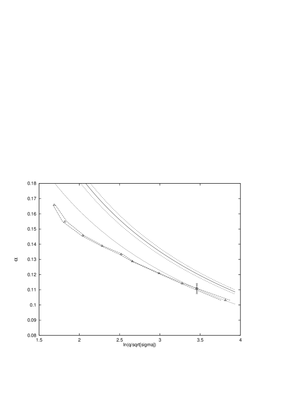
Figure 7: Comparison of three lattice predictions to $\alpha_{\overline{M\!S}}$ for $n_{f}=0$. The upper curve is from the present analysis, Eqs. (11,12). $\Delta$ : FNAL-$\overline{M\!S}$-scheme; $\Box$: result of Ref. [7] with its two-loop evolution (dotted line).

In Fig. 7, we display $\alpha_{\overline{M\!S}}$ vs.  $\ln q$, with the momentum in units of the string tension to avoid overall scale errors, in the zero flavour world. The upper error band refers to the two-loop evolution of our $\alpha_{q\bar{q}}$ values. Two sets of data are shown in comparison: the triangles refer to the estimates from Eq. (17), with $a$ determined from the string tension, while the point with error bar is the result of method (c), presented by WOLFF to this conference [7]. Note from Eq. (6) that our coupling scheme is much closer to the $\overline{M\!S}$ scheme than theirs, as expressed by the relation [7]

$$\alpha_{\overline{M\!S}}=\alpha_{C\!D\!M}+1.256\alpha^{2}_{C\!D\!M}+{\cal O}(\alpha^{3}_{C\!D\!M}).$$ (19)

6 UNQUENCHING

Having established the method in the pure gauge sector, we can now ask the sneaking question ‘what will happen in the real world with dynamical fermions present?’ In the absence of full fledged QCD simulations, we have to resort to sneaky answers, i.e. rough estimates [9] based on early day full QCD results.

For that purpose, we will exploit the work of the MT_c collaboration who performed a matching of the quenched and unquenched (4 flavour staggered fermions) potentials [21] by tuning $\beta$. Their results enable us to compute the FNAL-$\overline{M\!S}$ couplings, in the zero- and four- flavour worlds. From the latter, we can extract the matching of the accompanying $\Lambda$-values, and find $\Lambda_{\overline{M\!S}}^{(4)}=(.44\pm.10)\Lambda_{\overline{M\!S}}^{(0)}$. We assigned a $12\%$ ($10\%$) error due to matching ( scaling violation) uncertainties. The degeneracy of the lattice quarks leads us to increase the systematic error:

$$\Lambda_{\overline{M\!S}}^{(4)}=(.44^{+10}_{-14})\Lambda_{\overline{M\!S}}^{(0)}=129\pm 8^{+43}_{-60}\,\mbox{MeV}\quad.$$ (20)

This can be converted into an $\alpha$-value in the five flavour world at the $Z_{0}$ mass:

$$\alpha_{\overline{M\!S}}(m_{Z})=.1020^{+54}_{-104}\quad.$$ (21)

This lattice estimate appears to be rather low, compared to the average value from LEP experiments, which reads $\alpha_{\overline{M\!S}}^{\mbox{L}EP}=.118(7)$.

7 CONCLUSION

We have seen that a direct determination of the strong coupling from the interquark force is feasable with the computing power of an 8K Connection Machine CM-2. The final number for $\alpha_{s}(m_{Z})$, shown in Eq. (21), carries errors which are comparable to the experimental ones. At this stage, by far most of this estimated error is due to scale uncertainties ($15\%$ in $\Lambda^{n_{f}=0}_{\overline{M\!S}}$, mainly from quenching) and the cavalier $0\rightarrow 4$ flavour conversion ($30\%$).

The method is applicable to full QCD. Discretization effects can still be reduced in the present framework by going to finer lattices. Future effort should also go into the direction of a full lattice perturbative analysis.

References

- [1] A. and P. Hasenfratz, Phys. Lett. B93 (1980) 165; Nucl. Phys. B193 (1981) 210.
- [2] G.P. Lepage and P.B. Mackenzie, Nucl. Phys. B[Proc. Suppl.]20 (1991) 173; Phys. Rev. D48 (1993) 2250.
- [3] Ch. Michael, Phys. Lett. B283 (1992) 103.
- [4] G.S. Bali and K. Schilling, Phys. Rev. D47 (1993) 661; Nucl. Phys. B[Proc. Suppl.]30 (1993) 513.
- [5] M. Lüscher et al., Nucl. Phys. B384 (1992) 168.
- [6] M. Lüscher et al., Nucl. Phys. B389 (1993) 247; M. Lüscher et al., Nucl. Phys. B[Proc. Suppl.]30 (1993) 139.
- [7] U. Wolff, this volume; M. Lüscher et al., DESY preprint DESY-93-114 (1993).
- [8] A.X. El Khadra, this volume.
- [9] G.S. Bali, Wuppertal preprint WUB 93-37.
- [10] D. Barkai et al., Phys. Rev. D30 (1984) 1984.
- [11] M. Creutz, Phys. Rev. D21 (1980) 2308.
- [12] G.S. Bali and K. Schilling, Phys. Rev. D46 (1992) 2636.
- [13] S.P. Booth et al., Phys. Lett. B294 (1992) 385; Ch. Michael, Nucl. Phys. B[Proc. Suppl.]30 (1993) 509.
- [14] A. Billoire, Phys. Lett. B104 (1981) 472.
- [15] C.B. Lang and C. Rebbi, Phys. Lett. B115 (1982) 137.
- [16] R. Sommer, DESY preprint 93-062.
- [17] E. Eichten et al., Phys. Rev. D21 (1980) 203.
- [18] F. Butler et al, Phys. Rev. Lett. 70 (1993) 2849.
- [19] F. Karsch and R. Petronzio, Phys. Lett. B153 (1985) 87.
- [20] N. Stamatescu, this volume.
- [21] MTc Collaboration: K.D. Born et al., Nucl. Phys. B[Proc. Suppl.]26 (1992) 394; E. Laermann, private communication.