On Spin and Matrix Models in the Complex Plane

Abstract

We describe various aspects of statistical mechanics defined in the complex temperature or coupling-constant plane. Using exactly solvable models, we analyse such aspects as renormalization group flows in the complex plane, the distribution of partition function zeros, and the question of new coupling-constant symmetries of complex-plane spin models. The double-scaling form of matrix models is shown to be exactly equivalent to finite-size scaling of 2-dimensional spin systems. This is used to show that the string susceptibility exponents derived from matrix models can be obtained numerically with very high accuracy from the scaling of finite-$N$ partition function zeros in the complex plane.

                                                                                                         CERN–TH-6956/93                                                                                                          FSU-SCRI-93-87

1 Introduction

In contrast with what might be expected at first sight, the generalization of spin models and gauge theories to the complex activity [1] or temperature [2] plane is a subject rich in physical content. In general, information concerning the phase structure, and, in particular, the possible phase transitions for physical values of the parameters can be extracted from the behaviour of the finite volume partition function in the complex plane. The Yang-Lee edge singularity [1, 3] is one prime example of this, the predictions of the distribution of partition function zeros in the complex plane another [4]. That these beautiful results can also be very much of practical use in the study of phase transitions, has been amply demonstrated [5].

The purpose of this paper is to consider some aspects of spin, matrix and gauge theories in the complex plane that may have gone unnoticed until now. In so far as it is possible, we shall compare general predictions for the complex plane behaviour with exact analytical solutions. By doing so, we unravel various subtleties involved in defining these models for complex parameters, and we also gain additional insight into the nature of statistical mechanics off the real axis.

The simplest example of an exactly solvable model in statistical mechanics is the one-dimensional Ising model. Although this model cannot have a real phase transition at non-zero temperature, it does in fact have a continuous phase transition at $T=0$. Because of the special nature of a phase transition occurring at the origin, not all of the formalism of critical phenomena can directly be applied to this system. In particular, only certain ratios of critical exponents are uniquely defined. Nevertheless, this is often sufficient to test the more general predictions of complex plane partition functions. In section 2, we use this model to illustrate some of these more general results concerning the location of partition function zeros [4], and use it to comment on some interesting aspects of renormalization group flows in the complex plane. This is possible, since one can construct exact renormalization group transformations in the space of just three operators (the energy, the spin and the constant operator) by means of spin decimation.

In section 3 we turn to the question of new symmetries of discrete spin models at complex temperature, an issue recently brought up in the case of the Ising model by Marchesini and Shrock [6]. We show here that the non-trivial part of these new symmetries requires a careful definition of what is meant by the thermodynamic limit in the complex plane.

Section 4 contains a discussion of the double scaling limit in matrix models and a discussion of 2D $U(N)$ lattice gauge theory in the complex coupling constant plane. The parameter $N$, which eventually is sent to infinity in order to obtain a phase transition [7], is shown to play a rôle quite analogous to the volume in ordinary systems with a finite number of degrees of freedom per site (or plaquette). In this manner, we demonstrate that the double scaling of matrix models (and hence low-dimensional string theory) is nothing but ordinary finite-size scaling of models in statistical mechanics. This allows us to extract numerically the “string susceptibility” exponent of matrix models through the scaling of their corresponding partition function zeros. Finally, section 5 contains our conclusions.

2 The 1D Ising Model at Complex Activity and Complex Temperature

Define the partition function for a finite number of sites $N$ as

$${\cal Z}_{N}~{}=~{}\sum_{\sigma}{\rm e}^{K\sum_{j=1}^{N}\sigma_{j}\sigma_{j+1}+h\sum_{j=1}^{N}\sigma_{j}}~{},$$ (1)

with periodic boundary conditions, i.e.,$~{}\sigma_{N+1}=\sigma_{1}$. Introducing the symmetric transfer matrix $V(\sigma,\sigma^{\prime})$, it is trivial to compute the partition function from the trace:

$${\cal Z}_{N}~{}=~{}{\rm Tr}V^{N}~{}=~{}\lambda_{+}^{N}+\lambda_{-}^{N},$$ (2)

where $\lambda_{+}$ and $\lambda_{-}$ are the two eigenvalues. Noting that $V(\sigma,\sigma^{\prime})$ can be represented by a $2\times 2$ matrix,

$$V(\sigma,\sigma^{\prime}) = {\rm e}^{K\sigma\sigma^{\prime}+\frac{1}{2}(\sigma+\sigma^{\prime})}$$ (3)

$$= \left(\begin{array}[]{cc}{\rm e}^{K+h}&{\rm e}^{-K}\\ {\rm e}^{-K}&{\rm e}^{K-h}\end{array}\right)$$ (6)

one has

$$\lambda_{\pm}={\rm e}^{K}\cosh(h)\pm\sqrt{{\rm e}^{2K}\sinh^{2}(h)+{\rm e}^{-2K}}.$$ (7)

This is all well known. On the real axis $\lambda_{+}>\lambda_{-}$, and the thermodynamic limit of the partition function, reached as $N\to\infty$, involves only $\lambda_{+}$. For example, the free energy per spin is found to be

$$f=\lim_{N\to\infty}N^{-1}\ln{\cal Z}_{N}=\ln\lambda_{+}.$$ (8)

Similarly, the magnetization per spin is explicitly given by

$$m(h,K) ~{}=~{} \lim_{N\to\infty}N^{-1}{\cal Z}_{N}^{-1}\frac{\partial}{\partial h}\left[{\cal Z}_{N}\right]$$ (9)

$$~{}=~{} \frac{{\rm e}^{K}\sinh(h)}{[{\rm e}^{2K}\sinh^{2}(h)+{\rm e}^{-2K}]^{1/2}}.$$

It is also well-known that this system cannot have a phase transition for non-zero temperatures, and any real value of the magnetic field. We see this explicitly from the solution (8). Nevertheless, at $h=0$ the system does have a continuous phase transition at $T=0~{}(K=\infty)$, which to a very large extent can be phrased within the standard formalism of critical phenomena [8]. Since the transition occurs at an asymmetric point at which the usual scaled temperature variable $t=(T-T_{c})/T_{c}$ cannot be defined, one must be more careful and rewrite all scaling relations in terms of the correlation length. This in turn is computed from the 2-point function [9],

$$g_{ij}~{}\equiv~{}\langle\sigma_{i}\sigma_{j}\rangle-\langle\sigma_{i}\rangle\langle\sigma_{j}\rangle~{}=~{}\sin^{2}(2\phi)[\lambda_{+}/\lambda_{-}]^{|i-j|},$$ (10)

where $\phi$ is determined from the solution $0<\phi<\pi/2$ of $\cot(2\phi)={\rm e}^{2K}\sinh(h)$. This shows that

$$\xi=1/\ln[\lambda_{+}/\lambda_{-}],$$ (11)

which at $h=0$ is well-defined (and non-singular) for all positive temperatures. The usual critical exponents are then defined through the behaviour of the singular parts of the thermodynamic quantities as one approaches the critical point at $T=0$:

$$\Delta f(0,T)\sim\xi^{-(2-\alpha)/\nu}~{},~{}~{}~{}m(0,T)\sim\xi^{-\beta/\nu}~{},~{}~{}\chi(0,T)\sim\xi^{\gamma/\nu}.$$ (12)

From the exact solution (8) it follows that

$$\gamma=\nu=2-\alpha,$$ (13)

while from the corresponding exact solution of the 2-point function we see that $\eta=1$. Finally, from the behaviour of the magnetization at non-vanishing magnetic field at the critical point, $m(h,0)=sgn(h)$, it follows that $\delta=\infty$. Although this model does not display spontaneous magnetization, it follows from the definition (12) that $\beta=0$. These values of the critical exponents are all consistent with the general scaling relations

$$\alpha+2\beta+\gamma = 2$$ (14)

$$\beta\delta = \beta+\gamma$$ (15)

$$\gamma = (2-\eta)\nu$$ (16)

for $\beta\delta=\nu$ (a result which also follows formally from the exact solution given above), and with the general hyperscaling relation

$$d\nu = 2-\alpha$$ (17)

$$\delta = (d+2-\eta)/(d-2+\eta)$$ (18)

for $d=1$. Thus, although not all critical exponents are uniquely defined in this case, certain ratios of exponents are completely well defined, and in full accord with general scaling relations at a critical point.

These simple results do not hold in general, however, once we go off the real axis in either magnetic field $h$ (or activity ${\rm e}^{-2h}$) or temperature (proportional to $K^{-1}$). The reason is, of course, that the two transfer matrix eigenvalues $\lambda_{\pm}$ become in general complex-valued. The simple thermodynamic limit $N\to\infty$ then obviously does not always exist (if, $e.g.$, $|\lambda_{\pm}|=1$, the naive thermodynamic limit of the partition function is given by a non-convergent phase running around on the unit circle). But there are clearly also many regions in the complex plane where this naive thermodynamic limit is well-defined. The location of partition function zeros ${\cal Z}_{N}=0$ is one such example, which we turn to next.

One of the predictions of ref. [4] is that for a finite system of volume (number of sites) $N$, the partition function zeros close to the critical point should scale as

$$h_{n}^{2}~{}=~{}N^{-2\beta\delta/\nu}f_{n}(0),$$ (19)

where the index $n$ indicates the $n$th partition function zero. Also, the scaling function $f_{n}(KN^{1/\nu})$ evaluated at zero argument has been predicted to behave, for $n$ large, like [4]

$$f_{n}(0)~{}=~{}-Cn^{2\delta/(\delta+1)},$$ (20)

where $C$ is some constant. In other words, close to the critical point we should have

$$h_{n}^{2}~{}=~{}-CN^{-2\beta\delta/\nu}n^{2\delta/(\delta+1)},$$ (21)

which in the case of the 1D Ising model unambiguously implies

$$h_{n}~{}=~{}iC^{1/2}\frac{n}{N}.$$ (22)

Let us compare this with the known exact solution. In the limit $K>>1$, it follows from eq. (7) that

$$\lambda_{+} ~{}=~{} {\rm e}^{K}\cosh(h)+{\rm e}^{K}\sinh(h)$$ (23)

$$\lambda_{-} ~{}=~{} {\rm e}^{K}\cosh(h)-{\rm e}^{K}\sinh(h).$$ (24)

Thus, in this limit we see from eq. (2) that

$${\cal Z}_{N}~{}\sim~{}2{\rm e}^{NK}\cosh(Nh).$$ (25)

The partition function zeros are therefore to be found at

$$h_{n}~{}=~{}\frac{i\pi}{2N}(2n+1),$$ (26)

or, since $n$ should be taken large in order to compare with eq. (22),

$$h_{n}~{}\sim~{}i\pi\frac{n}{N},$$ (27)

which is precisely the expected behaviour (22), with $C=\pi^{2}$.

In the 2D Ising model the partition function zeros at zero magnetic field lie on two intersecting circles in the complex temperature plane [2]. One of these circles crosses the real temperature axis at the 2D Ising critical temperature $T_{c}$ at a right angle. For the 1D Ising model it follows from eq. (2) that the zero-field partition function zeros lie on just one circle, the unit circle in the complex $\tanh(K)$-plane, crossing the real axis at $\tanh(K)=1$ (corresponding to the 1D Ising critical coupling $K=\infty$) again at a right angle. Although not rigorously related to the general prediction for this angle $\varphi$ of ref. [4]:

$$\tan[(2-\alpha)\varphi]~{}=~{}\frac{\cos(\pi\alpha)-A_{-}/A_{+}}{\sin(\pi\alpha)},$$ (28)

this behaviour is at least consistent with it. Here $\alpha$ is the usual critical exponent, and $A_{\pm}$ are the specific heat amplitudes above and below $T_{c}$. For $\varphi=\pi/2$ eq. (28) can be brought to

$$[1-A_{-}/A_{+}]\cos(\alpha\pi)=-[1-A_{-}/A_{+}].$$ (29)

Solutions are either $\alpha=1$ with $A_{-}/A_{+}$ undetermined or $A_{-}/A_{+}=1$ with $\alpha$ undetermined. The latter agrees with what we previously found and hence the prediction (28) applies to the 1D Ising model.

2.1 Complex-plane Singularities of the 1D Ising Model

Let us define a “ critical point” anywhere in the complex plane by the condition of a diverging correlation length, $\xi=\infty$. In the 1D Ising model we have already seen that $\xi=1/\ln[\lambda_{+}/\lambda_{-}]$, where $\lambda_{\pm}$ are the two transfer matrix eigenvalues. The condition $\xi=\infty$ in this case implies $\lambda_{+}=\lambda_{-}$. When $h=0$, this gives

$$\cosh(K)~{}=~{}\sinh(K),$$ (30)

which for real $K$ can only be satisfied asymptotically at $K=\infty$. This is just the usual 1D Ising transition at $T=0$.

When $h\neq 0$, there are more possibilities. In particular, $\lambda_{+}=\lambda_{-}$ in the whole subspace where

$${\rm e}^{2K}\sinh^{2}(h)+{\rm e}^{-2K}~{}=~{}0.$$ (31)

Consider first a simple special case, where $K$ is real, but $h$ is allowed to become complex. Then, parametrizing $h=h_{1}+ih_{2}$, and using some trigonometric identities, we find that vanishing of the imaginary part of eq. (31) implies

$$2{\rm e}^{2K}\sinh(h_{1})\cos(h_{2})\cosh(h_{1})\sin(h_{2})~{}=~{}0,$$ (32)

$i.e.,~{}h_{1}=0$, or $h_{2}=n\pi/2$ or both. Demanding also the vanishing of the real part of eq. (31) thus splits up in two parts: (a) $h_{1}=0$ and (b) $h_{2}=n\pi/2$. Case (a) implies

$$\sin^{2}(h_{2})~{}=~{}\exp[-4K],$$ (33)

which can only be satisfied for $K>0$. The solution to this equation in the complex ${\rm e}^{h}$-plane is shown graphically in fig. 1a.

Figure 1: Critical points for the 1D Ising model with complex couplings.

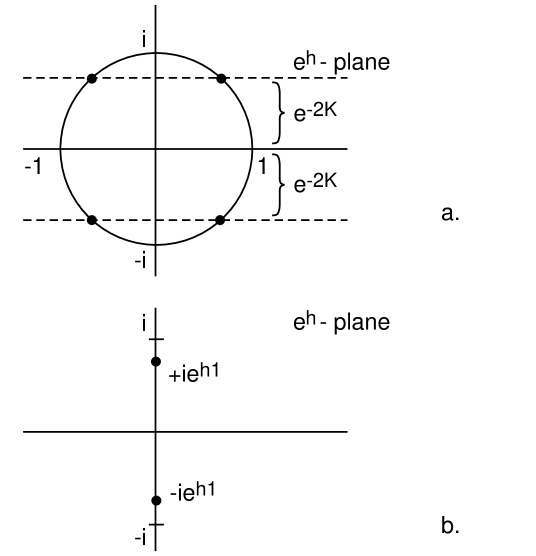
Case (b) leads to

$${\rm e}^{2K}\left\{\sinh^{2}(h_{1})\cos^{2}\left(\frac{n\pi}{2}\right)-\cosh^{2}(h_{1})\left[1-\cos^{2}\left(\frac{n\pi}{2}\right)\right]\right\}+{\rm e}^{-2K}~{}=~{}0,$$ (34)

which in turn has two possible solutions. In the first case, $\cos^{2}(n\pi/2)=+1$, for which the above equation reduces to ${\rm e}^{2K}\sinh^{2}(h_{1})+{\rm e}^{-2K}=0$. This cannot be satisfied for real $h_{1}$ and $K$. The other case is $\cos^{2}(n\pi/2)=0,~{}i.e.~{}n=(2j+1),~{}j=0,1,\ldots$, which leads to

$$\cosh^{2}(h_{1})~{}=~{}\exp[-4K].$$ (35)

Although this equation cannot be satisfied for $K>0$, there are non-trivial solutions for $K<0$, which we can think of as the antiferromagnetic situation. In the complex ${\rm e}^{h}$-plane this corresponds to the solutions shown in fig. 1b.

At these points in the complex plane we have not only $\xi=\infty$, but also magnetization $m=\infty$. The finite volume partition function in these cases equals

$${\cal Z}_{N}~{}=~{}2[{\rm e}^{K}\cosh(h)]^{N},$$ (36)

so that, on account of $\cosh(h_{1}+ih_{2})=\cosh(h_{1})\cos(h_{2})+i\sinh(h_{1})\sin(h_{2})$, the case (a) corresponds to ${\cal Z}_{N}$ real. In contrast, in the antiferromagnetic case of (b), $\lambda_{+}=\lambda_{-}$ are purely imaginary. The simplest thermodynamic limit $N\to\infty$ does not exist in this case.

On viewing the above results, one question that immediately arises is: how can a local quantity such as the magnetization per spin diverge at these complex-plane critical points?

To answer this question in detail, let us try to regularize everything by considering first a finite volume of $N$ spins. We still have

$$m(h,K)~{}\equiv~{}{\cal Z}_{N}^{-1}\frac{\partial}{\partial h}\left\{\frac{{\cal Z}_{N}}{N}\right\},$$ (37)

but now both transfer matrix eigenvalues must be kept in the expression for the partition function, $i.e.~{}{\cal Z}_{N}=\lambda_{+}^{N}+\lambda_{-}^{N}$. Carrying out the differentiation, a convenient way to express the finite-volume magnetization is as

$$m(h,K)~{}=~{}\frac{{\rm e}^{K}\sinh(h)}{[{\rm e}^{2K}\sinh^{2}(h)+{\rm e}^{-2K}]^{1/2}}~{}\frac{\lambda_{+}^{N}-\lambda_{-}^{N}}{\lambda_{+}^{N}+\lambda_{-}^{N}}.$$ (38)

Ordinarily, on the real axes, $\lambda_{+}>\lambda_{-}$, in which case the above expression reduces in the thermodynamic limit $N\to\infty$ to the magnetization $m(h,K)$ of eq. (9). But the present case corresponds to $\lambda_{+}=\lambda_{-}$, so we must be more careful. If we take the limit $\lambda_{-}\to\lambda_{+}$ (where ${\rm e}^{2K}\sinh^{2}(h)+{\rm e}^{-2K}\to 0$) for any finite $N$, then

$$\lambda_{+}^{N}-\lambda_{-}^{N}~{}\simeq~{}[{\rm e}^{K}\cosh(h)]^{N-1}\times 2N\times({\rm e}^{2K}\sinh^{2}(h)+{\rm e}^{-2K})^{1/2},$$ (39)

while of course

$$\lambda_{+}^{N}+\lambda_{-}^{N}~{}\simeq~{}2[{\rm e}^{K}\cosh(h)]^{N}$$ (40)

to lowest order. Thus at any finite $N$ we have

$$m(h,K)=\frac{N{\rm e}^{K}\sinh(h)}{{\rm e}^{K}\cosh(h)}=N\tanh(h)$$ (41)

at these complex-plane critical points. This behaviour, linear growth with the size of the system, is actually precisely as expected from finite-size scaling theory when we treat these complex-plane singularities as true critical points. To see this, consider again the infinite-volume magnetization at, for simplicity, purely imaginary external magnetic field $h=ih_{2}$,

$$m(h_{2},K)=\frac{ie^{K}\sin(h_{2})}{[e^{-2K}-\sin^{2}(h_{2})e^{2K}]^{1/2}}~{}.$$ (42)

Expanding $h_{2}=h_{2}^{*}+\Delta h_{2}$ around a critical magnetic field $h_{2}^{*}$ given by $\sin^{2}(h_{2}^{*})=\exp[-4K]$, we note that

$$m(\Delta h_{2},K)~{}\sim~{}\Delta h_{2}^{\rho}$$ (43)

as $\Delta h_{2}\to 0$, with $\rho=-1/2$.

Similarly, for the correlation length we have

$$\xi^{-1}=\ln\left[\frac{\lambda_{+}}{\lambda_{-}}\right]=\ln\left[\frac{e^{K}\cos(h_{2}^{*})+c\sqrt{\Delta h_{2}}}{e^{K}\cos(h_{2}^{*})-c\sqrt{\Delta h_{2}}}\right]~{}\sim~{}\Delta h_{2}^{\nu}~{},$$ (44)

with $\nu=1/2$. Finite-size scaling theory [10] then predicts

$$m(\Delta h_{2},K)~{}\sim~{}N^{-\rho/\nu}~{}\sim~{}N~{},$$ (45)

in agreement with the explicit solution (41).

2.2 Renormalization Group Flows in the Complex Plane

Not surprisingly, the 1D Ising model can be solved by an exact real-space renormalization group transformation, spin decimation. This hence gives us the possibility of explicitly observing some exact results concerning RG flows in the complex plane, results that cannot easily be obtained from more general principles. For a rescaling factor $b=2$, the exact RG transformation for the 1D Ising model takes the following form [8]:

$$\exp[4K^{\prime}] ~{}=~{} \frac{\cosh(2K+h)\cosh(2K-h)}{\cosh^{2}(h)}$$

$$\exp[2h^{\prime}] ~{}=~{} {\rm e}^{2h}~{}\frac{\cosh(2K+h)}{\cosh(2K-h)},$$ (46)

where primed variables are the renormalized couplings. The RG flow in the $K-h$ plane is not trivial [3], but when $h=0$ it becomes very simple: we get $\exp[2h^{\prime}]=1,~{}i.e.~{}h^{\prime}=0$. This just expresses consistency; when we start with no magnetic field, we do not generate it in the process of renormalization. The flow in the temperature direction is slightly less trivial:

$${\rm e}^{4K^{\prime}}~{}=~{}\cosh^{2}(2K).$$ (47)

This equation has two fixed points, $K^{*}=0$ and $K^{*}=\infty$. The fixed point at $K^{*}=\infty$ is unstable, and it is the usual 1D Ising critical point; here $\xi=\infty$.

Now, from general principles the infinite correlation length condition $\xi=\infty$, which is fulfilled on the surface

$$\sinh^{2}(h)~{}=~{}-{\rm e}^{-4K},$$ (48)

must be associated with a “critical hypersurface” in the complex plane. Once on this surface, the RG flow must remain on it. It is easy to verify that

$${\rm e}^{-4K^{\prime}} ~{}=~{} -\sinh^{2}(h^{\prime})~{}~{}~{}{\mbox{\rm if and only if}}$$ (49)

$${\rm e}^{-4K} ~{}=~{} -\sinh^{2}(h).$$ (50)

Note that this complex-plane hypersurface intersects the plane with real couplings $K$ and $h$ at the usual critical point $(K,h)=(\infty,0)$, so we should expect that this surface in almost all respects can be treated as a standard critical hypersurface. (There should then also be complex-plane equivalents of irrelevant operators, pushing the RG flow towards a fixed point on this surface).

It follows from eqs. (46) that the critical surface given by (48) contains, besides the unstable fixed point $(K,h)=(\infty,0)$, two stable ones at $(K,h)=(0,\pm i\pi/2)$ (everything is symmetric under $h\to-h$). The critical line in the interesting coupling plane $({\rm e}^{-K},ih_{2})$ and the RG flow on it are shown in fig. 2. The figure also shows the results of iterating the RG equations starting at several points a little off of the critical line.

Figure 2: Renormalization group flow for the 1D Ising model in the plane ${\rm e}^{-K}$ and $h=ih_{2}$. The critical line is shown with the direction of flow indicated. Some results from iterating the RG away from the critical line are also given with different plotting symbols and connected with dotted lines to guide the eye. The flow is always away from the origin.

What about the zeros of ${\cal Z}_{N}$? Let us start with a lattice of couplings $(K,h=0)$ and a number of sites equal to $2N$, and then apply the RG transformation of rescaling factor 2. The zeros of ${\cal Z}_{2N}$ are given by

$$\frac{{\rm e}^{K}-{\rm e}^{-K}}{{\rm e}^{K}+{\rm e}^{-K}}~{}=~{}{\rm e}^{i\pi(2n+1)/2N},$$ (51)

and squaring this, we get successively

$${\rm e}^{i\pi(2n+1)/N} ~{}=~{} \left(\frac{{\rm e}^{K}-{\rm e}^{-K}}{{\rm e}^{K}+{\rm e}^{-K}}\right)^{2}$$ (52)

$$~{}=~{} \frac{\cosh(2K)-1}{\cosh(2K)+1}$$ (53)

$$~{}=~{} \frac{\cosh^{1/2}(2K)-\cosh^{-1/2}(2K)}{\cosh^{1/2}(2K)+\cosh^{-1/2}(2K)}$$ (54)

$$~{}=~{} \frac{{\rm e}^{K^{\prime}}-{\rm e}^{-K^{\prime}}}{{\rm e}^{K^{\prime}}+{\rm e}^{-K^{\prime}}}.$$ (55)

The zeros of the partition function thus behave as expected under this exact RG transformation: the zeros of ${\cal Z}_{2N}$ move to those of ${\cal Z}_{N}$.

The RG flow in the complex plane is therefore far from smooth, and except for the neighbourhood of the critical hypersurface discussed above, it does not much resemble the usual RG flows for real couplings. Consider plotting the flow in the complex $\tanh(K)$-plane. On the unit circle of this plane the partition function zeros jump around corresponding to going from $\exp[i\pi(2n+1)/2N]$ to $\exp[i\pi(2n+1)/N]$ as $K$ goes into $K^{\prime}$. But in the ordinary coupling constant plane of $K$, this means going from, for example in the last case $N=1$: $K=\pm i\pi/4$ to $K^{\prime}=-\infty$ in one RG step.

2.3 The Generalized Heisenberg Model

The partition function

$${\cal{Z}}_{N}~{}=~{}\sum_{\vec{\sigma}}e^{K\sum_{j=1}^{N}\vec{\sigma}_{j}\cdot\vec{\sigma}_{j+1}+\sum_{j=1}^{N}\vec{h}\cdot\vec{\sigma}_{j}}$$ (56)

defines a natural generalization of the 1D Ising model, – the generalized Heisenberg model in 1D. Here $\vec{\sigma}_{i}$ denotes an $n$-dimensional vector of unit length, and $\vec{h}$ is a vector of fixed orientation (which can be chosen at will) describing an external magnetic field. For $n=1$ this reduces to the ordinary 1D Ising model, while the cases $n=2$ and $n=3$ correspond to the planar and original classical Heisenberg model, respectively. The model is solvable for all $n$ in one dimension when the external field vanishes [11]. We shall here use this exact solution to reinvestigate complex-temperature partition functions.

The eigenvalues of the transfer matrix of eq. (56) are known in closed analytical form [11, 12]:

$$\lambda_{i}~{}=~{}(2\pi)^{\frac{1}{2}n}K^{1-\frac{1}{2}n}I_{\frac{1}{2}n-1+i}(K),$$ (57)

where $i=0,1,\ldots$, and $I_{\nu}(x)$ is the modified Bessel function of order $\nu$. The model can be studied straightforwardly for integer values of $n$, in which case it yields only small modifications in comparison with the Ising case. (The phase transition temperature remains at $T_{c}=0$, the critical indices being equal to the Ising indices for all finite values of $n$.) What is more interesting for our purpose here is that the model also admits a unique analytic continuation in $n$ for $0<n<1$ [12]. In this case the phase transition takes on a more familiar form, occurring now at a finite value of $T_{c}$. The correlation function is determined by the two leading transfer matrix eigenvalues, and reads explicitly

$$\langle\vec{\sigma}_{i}\vec{\sigma}_{j}\rangle~{}=~{}\left[\frac{I_{\frac{1}{2}n}(K)}{I_{\frac{1}{2}n-1}(K)}\right]^{|i-j|}.$$ (58)

This corresponds to a correlation length

$$\xi^{-1}~{}=~{}\ln\left[\frac{I_{\frac{1}{2}n}(K)}{I_{\frac{1}{2}n-1}(K)}\right]{}~{},$$ (59)

which diverges at the phase transition point $K_{c}$ determined by

$$I_{\frac{1}{2}n}(K_{c})~{}=~{}I_{\frac{1}{2}n-1}(K_{c}).$$ (60)

As mentioned above, this phase transition occurs at a finite value of $K_{c}$ when $0<n<1$. The condition of a diverging correlation length,

$$|I_{\frac{1}{2}n}(K_{c})|~{}=~{}|I_{\frac{1}{2}n-1}(K_{c})|,$$ (61)

continued into the complex plane thus reduces as $n\to 1$ to the circle $|coth(K)|=1$ of the 1D Ising model.

Having solvable models with a finite critical point $K_{c}$, we can investigate the finite-size scaling of the zeros of the partition function in the complex plane [4]. The zero closest to the real axis should approach the critical point $K_{c}$ at a rate determined by the correlation length exponent $\nu$

$${\mbox{\rm Im}}(K_{0})\propto N^{-1/\nu}~{}.$$ (62)

As an example we consider $n=0.5$ with the critical point at $K_{c}=0.6755198$. The scaling (62) is shown in fig. 3. From two successive sizes, we can get an estimate $\nu(N)$ of $\nu$. These estimates are given in table 1.

Figure 3: Finite size scaling of the complex partition function zero closest to the real axis for the $n=0.5$ 1D Heisenberg model.

Table 1: Estimates of $\nu$ from the finite scaling of the imaginary part of the partition function zeros computing from successive $N$ (second column) and extrapolated to $N=\infty$ from two successive estimates (third column).

$N$	$\nu(N)$	$\nu(\infty)$
8	3.168120
12	1.998528	1.062855
16	1.587125	1.058179
20	1.385652	1.027478
24	1.271576	1.012312
28	1.200939	1.005329
32	1.154338	1.002107
36	1.122063	1.000559
40	1.098848	0.999877
48	1.075312	1.021823
56	1.054356	0.996325
64	1.041037	0.997529
72	1.032060	0.998264
80	1.025729	0.998739

We can see that the estimates for $\nu$ are already quite close to the known exact value $\nu=1$ [12]. Assuming a finite-size correction of the form $N^{-2}$, which fits the data best, we can get infinite volume estimates from two successive estimates $\nu(N)$. These estimates for $\nu$, also given in table 1, are remarkably good.

3 New Symmetries of Spin Models

In a very interesting paper, Marchesini and Shrock [6], have recently derived what is apparently new symmetries of the zero-field Ising model in any number of dimensions. The symmetries are related to discrete transformations of the Ising coupling constant (or temperature) in the complex temperature plane. Evidence was found that these new symmetries are not without influence on results derived for real coupling constants, since they also signal new singularities in the complex plane, singularities that may affect $e.g.$ Padé approximants of truncated series expansions on the real coupling constant axis. The symmetries, although clearly not of universal nature, are generalizable to other discrete spin models. Again, let us consider these general results in the light of the simple solvable 1D Ising model. We shall later make some related remarks on the 2D Ising case.

The 1D Ising model is of coordination number $q=2$, and the two main theorems of ref. [6] are therefore applicable in this case. These state that the zero-field ($h=0$) free energy $f(K)$ should be invariant under the following transformations:

$$f(K) ~{}=~{} f(K+in\pi)~{},~{}~{}~{}n~{}{\mbox{\rm integer}}$$ (63)

$$f(K) ~{}=~{} f\left(K+i\left(n+\frac{1}{2}\right)\pi\right)~{},~{}~{}~{}n~{}{\mbox{{\rm integer}}}.$$ (64)

But if we take the explicit expression for the free energy per spin of the 1D Ising model,

$$f(K)~{}=~{}-\ln[2\cosh(K)],$$ (65)

this does not appear to be satisfied. In fact, the only invariance of this kind in eq. (65) is

$$K~{}\to~{}k+2\pi in~{},~{}~{}~{}n~{}{\mbox{\rm integer}},$$ (66)

which is trivially satisfied by the Ising model in any number of dimensions, on account of the integer-valued nature of the spin-spin interaction. How can we understand this discrepancy?

The explanation lies, of course, in the subtlety involved in defining the thermodynamic limit of the partition function off the real axis. In defining the free energy of the infinite volume Ising model as in eq. (65) above, we have already chosen one particular limit, the one valid on the real coupling constant axis. Although this expression can be analytically continued into the complex plane, the resulting free energy may not be derivable from the infinite volume limit of the general partition function in the complex plane. As we have already seen in several examples before, these two procedures do not always commute.

To understand the new symmetry, let us therefore revert to the finite volume partition function ${\cal Z}_{N}=\lambda_{+}^{N}+\lambda_{-}^{N}$. With zero magnetic field,

$$\lambda_{+}~{}=~{}2\cosh(K)~{},~{}~{}~{}~{}\lambda_{-}~{}=~{}2\sinh(K),$$ (67)

and consider now the transformation (64). Under this,

$$\cosh(K) ~{}\to~{} (-1)^{n}i\sinh(K)$$ (68)

$$\sinh(K) ~{}\to~{} (-1)^{n}i\cosh(K),$$ (69)

or in other words,

$$\lambda_{+}~{}\to(-1)^{n}i\lambda_{-}~{},~{}~{}~{}~{}\lambda_{-}~{}\to~{}(-1)^{n}i\lambda_{+}.$$ (70)

Consider now taking the thermodynamic limit in steps of $4N$ instead of just in steps of $N$, as it is usually defined. Then, with $\tilde{N}=4N$, the transformation (64) acts on the partition function as

$${\cal Z}_{\tilde{N}} ~{}=~{} \lambda_{+}^{4N}+\lambda_{-}^{4N}$$ (71)

$$~{}\to~{} [(-1)^{n}i\lambda_{-}]^{4N}+[(-1)^{n}i\lambda_{+}]^{4N}$$ (72)

$$~{}=~{} \lambda_{-}^{4N}+\lambda_{+}^{4N}~{}=~{}{\cal Z}_{\tilde{N}},$$ (73)

which shows explicitly that this indeed is a symmetry; the transformation has not done more than what effectively amounts to swapping eigenvalues.

But here another subtlety in connection with this new symmetry becomes apparent: it is not sufficient to remain at the level of finite volume partition functions, perform the transformation, and then take the thermodynamic limit. Instead, the symmetry hinges in an essential way on the precise definition of boundary conditions and the very manner in which this thermodynamic limit is defined. On the real axis these problems usually do not arise; one obtains a unique thermodynamic limit independently of the manner in which the thermodynamic limit is reached. In the complex plane the final thermodynamic quantities depend on the way in which the infinite volume limit is taken. From a physical point of view this is not acceptable: we must obtain the same bulk thermodynamic quantities no matter how we take the infinite volume limit. But again, this problem fortunately only surfaces once we enter unphysical parameter values! The need to take the thermodynamic limit in units of $4N$ instead of $N$ was noticed already in ref. [6], and in fact (as expected from the example shown above), plays a highly non-trivial rôle in the proof. The problem involved in taking the simplest infinite volume limit $N\to\infty$ off the real axis becomes apparent if we consider the coupling constant values $K+i(n+1/2)\pi$ discussed above. If we just let $N\to\infty$, the partition function becomes a non-convergent oscillatory number proportional to $e^{iN\pi/2}$.

The same remarks hold for other quantities, but not always with the same restriction on only considering a particular thermodynamic limit. For example, although the correlation length $\xi=1/\ln[\lambda_{+}/\lambda_{-}]$ does change under the transformation (64), the real part of its analytic continuation into the complex plane remains invariant. Thus, Re($\xi^{-1})=0$ not only at the usual critical point(s), but also at all points in the complex plane connected through the transformation (64). It was noted in ref. [6] that for the 2D Ising model the condition Re$(\xi^{-1})=0$ is fulfilled on the same points in the complex plane where the partition function vanishes. This is actually no accident, occurring because $\xi\propto 1/\ln[\lambda_{1}/\lambda_{0}]$, where $\lambda_{1,0}$ are the two leading eigenvalues of the 2D Ising transfer matrix [13]. Since the 2D Ising partition function also acquires its zeros when $|\lambda_{0}|=|\lambda_{1}|$, this is the rationale for the equality of these two sets. This particular mechanism, degeneracy of two (or more) leading transfer matrix eigenvalues, behind both partition function zeros and the condition Re$(\xi^{-1})=0$, is in fact more general [14]. It occurs in the 1D Ising model as well. Here, without a magnetic field, the condition Re$(\xi^{-1})=0$ implies

$$|\coth(K)|~{}=~{}1,$$ (74)

while the zeros of ${\cal Z}_{N}$ are found at

$$\lambda_{+}/\lambda_{-}~{}=~{}e^{i\pi(2n+1)/N},$$ (75)

$i.e.$, for the $N\to\infty$ limit again given by the unit circle $|\coth(K)|=1$. In fact, it is precisely because it is also a partition function zero that the condition Re$(\xi^{-1})=0$ in the complex plane can be associated with an unambiguous thermodynamic limit.

Similarly, the transformation (63) also only defines a real symmetry of the 1D Ising model if a very particular definition of the thermodynamic limit is used. The case $n=$ even is trivial, so we need only consider the case $n=$ odd, $i.e.:~{}K\to K+(2n+1)i\pi$. Under this transformation, $\lambda_{\pm}~{}\to~{}-\lambda_{\pm},$ and the partition function is symmetric if one takes the thermodynamic limit in units of $2N$. (Because the coordination number is $q=2$, there is no need to take the thermodynamic limit in multiples of $4N$; this also follows from the general proof in ref. [6]).

The existence of these kinds of symmetries appears to have been known for some time by practitioners of transfer matrix techniques (see, $e.g$, chapter 7 of ref. [9]).

4 The Double-Scaling Limit: Matrix Models

The non-analytic behaviour around phase transitions always arises as a result of a singular procedure, the thermodynamic limit, in which the number of degrees of freedom diverges. For a finite number of degrees of freedom, the partition function is an analytic of the coupling (or temperature). It is well known that a thermodynamic limit can be achieved not only by letting the volume (or number of sites) go to infinity, but also in finite volumes (or even on just points, $i.e.$ zero dimensional field theories) provided the number of degrees of freedom diverges by some other means. One example of this is large-$N$ matrix models in zero dimensions, which can display behaviour completely analogous to ordinary infinite-volume phase transitions. Another classical example is two-dimensional QCD in the $N\to\infty$ limit. By gauge invariance, two-dimensional latticized $SU(N)$ Yang-Mills theory is a one-plaquette theory. This “trivial” theory with Wilson action nevertheless undergoes a 3rd order phase transition in the limit $N=\infty$ [7]. One curious aspect of this 3rd order Gross-Witten transition is that the correlation length, defined in a natural physical way as

$$\xi\sim\sigma^{-1/2},$$ (76)

where $\sigma$ is the string tension, remains finite at the phase transition. This is difficult to reconcile with renormalization group ideas that seem to always require some diverging correlation length at non-trivial fixed points. Does this mean that the Gross-Witten phase transition cannot be understood from a renormalization group perspective? Or do we just have to search a little more for the true underlying correlation length that diverges at the transition?

The purpose of this section is therefore threefold. First, we shall analyze the matrix model phase transitions from the point of view of scaling of partition function zeros. Second, we shall answer the question: What is the analogue of the “double scaling limit” [15] of such matrix models [16] in ordinary systems in statistical mechanics? And third, we shall describe the appropriate renormalization group scenario for the Gross-Witten transition (which actually does correspond to a diverging correlation length, to be defined shortly).

We start with the last two questions, which turn out to be intimately related. But first a few definitions: By the double scaling limit of matrix models (and low-dimensional string theory) we mean the following. The singular part of the string partition function $\zeta(\Lambda,{\cal{G}})$ (a somewhat confusing terminology in this context, since it will be identified with the free energy of certain matrix models) scales as [17]:

$$\zeta(\Lambda,{\cal{G}})\sim(\Lambda^{*}-\Lambda)^{2-\gamma_{0}}\sum_{G=0}^{\infty}a_{G}\left[(\Lambda^{*}-\Lambda){\cal{G}}^{-2/\gamma_{1}}\right]^{G},$$ (77)

where the sum runs over genus $G$. Since the same factor appears for all genera, this means that

$$\zeta(\Lambda,{\cal{G}})\sim(\Lambda^{*}-\Lambda)^{2-\gamma_{0}}F((\Lambda^{*}-\Lambda){\cal{G}}^{-2/\gamma_{1}})~{},$$ (78)

where the scaling function $F$ is simply the sum on the r.h.s. of eq. (77). Here $\Lambda$ is the cosmological constant, and ${\cal{G}}$ is the string coupling constant. The exponents $\gamma_{0}$ and $\gamma_{1}$ are known from continuum calculations [17]:

$$\gamma_{1} = \frac{1}{12}\left[25-c+\sqrt{(1-c)(25-c)}\right]$$ (79)

$$\gamma_{0}+\gamma_{1} = 2,$$ (80)

where $c$ is the central charge. We shall mostly consider the simple case $c=0$, which corresponds to zero-dimensional matrix models.

In such a matrix model representation, $(\Lambda^{*}-\Lambda)\sim(g^{*}-g)$ and ${\cal{G}}\sim 1/N$, where $g$ is the matrix model coupling constant, and $N$ is the size of the matrix. The double scaling limit entails sending $g\to g^{*}$, the critical point of the matrix model at $N=\infty$, while simultaneously sending $N\to\infty$ in such a manner that the scaling variable

$$x=(g-g^{*})N^{2/\gamma_{1}}$$ (81)

is kept fixed.

Figure 4: Illustration of a real-space renormalization group transformation.

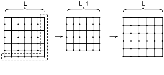
What is the analogue of this double scaling limit in ordinary spin systems? It turns out to be useful to think of a system at finite size $L$, $i.e.$, volume $V=L^{d}$ in $d$ dimensions. A two-dimensional analogue of such a system is shown in fig. 4. Now let us perform a simple real-space renormalization group transformation in the form of a spin decimation. Wishing to retain the same geometry (although in rescaled form), we choose to integrate out all spins along one row and one column, as also indicated in fig. 4. Let us denote the spins we integrate out by $\phi$, and the remaining ones by $\phi^{\prime}$. This spin decimation induces a renormalization group flow; the original Hamiltonian $H$ of operators ${\cal{O}}_{i}$ and corresponding coupling constants $g_{i}$ is mapped into a new Hamiltonian $H^{\prime}$ with in general new interactions ${\cal{O}}^{\prime}_{i}$, and in any case new coupling constants $g_{i}^{\prime}$. That is,

$${\rm e}^{L^{d}G(g)}\int d\phi^{\prime}{\rm e}^{-H^{\prime}(\phi^{\prime},g^{\prime})}=\int d\phi^{\prime}d\phi{\rm e}^{-H(\phi,\phi^{\prime},g)}~{},$$ (82)

where we have explicitly, as is customary, extracted the constant part $G(g)$ of the new Hamiltonian. Defining the free energy by

$$f(g)\equiv\frac{1}{L^{d}}\ln{\cal{Z}}(g),$$ (83)

this indeed corresponds to the standard real-space renormalization group equation for $f$,

$$f(g)=G(g)+b^{-d}f(g^{\prime})$$ (84)

with a length rescaling factor

$$b=\frac{L}{L-1}.$$ (85)

But this time this equation has the meaning of a finite-size renormalization relation. In the limit of large volume, $L\to\infty$, the number of spins integrated out at each step compared with the number of those retained becomes infinitesimal. This allows us to phrase the real-space renormalization group equation in infinitesimal form, giving in effect a Callan-Symanzik–type equation for finite-size scaling.

The constant part $G(g)$ of the Hamiltonian is assumed to be regular. We write it as

$$G(g)=\ln[\lambda(g)]$$ (86)

where $\lambda(g)$ must approach unity for large $L$:

$$\lambda(g)=1+\frac{1}{L}r(g)+{\cal{O}}\left(\frac{1}{L^{2}}\right).$$ (87)

Similarly, for large $L$, the coupling constants $g_{i}^{\prime}$ will be close to the previous values $g_{i}$, so that we may define functions $\beta_{i}(g_{i})$ by

$$g_{i}^{\prime}=g_{i}+\frac{1}{L}\beta_{i}(g_{i})+{\cal{O}}\left(\frac{1}{L^{2}}\right).$$ (88)

It is then straightforward to see that the recursion relation

$$[\lambda(g)]^{L^{d}}{\cal{Z}}(L-1,g^{\prime})={\cal{Z}}(L,g)$$ (89)

for the partition function implies the following differential equation for the free energy $f(L,g)$:

$$\left[L\frac{\partial}{\partial L}-\sum_{i}\beta_{i}(g_{i})\frac{\partial}{\partial g_{i}}+d\right]f(L,g)=r(L,g).$$ (90)

This is the Callan-Symanzik equation for finite-size scaling. The $\beta$-functions $\beta_{i}(g_{i})$ have been used by Roomany and Wyld [18] (see also ref. [10]) to get infinite-volume results from finite-size scaling. Their main advantage is that they have zeros even in finite volumes, where no phase transitions can occur. The zeros of these $\beta$-functions determine the location of the phase transitions in the infinite-volume systems.

The Callan-Symanzik equation (90) above gives an exact differential equation for the free energy $f(L,g)$ for all values of the couplings $g_{i}$ in the limit of infinite volume, $L\to\infty$. It is not restricted to the critical regime close to a critical point given by $\{g_{i}^{*}\}$.

For large but finite volumes $L^{d}$, we can extract the singular behaviour of the free energy near the infinite-volume fixed point $\{g_{i}^{*}\}$. For simplicity, assume that we have only one coupling constant $g$. Define an ordinary critical point $g^{*}$ by a solution of

$$\beta(g^{*})=0~{},~{}~{}~{}~{}~{}\beta^{\prime}(g^{*})>0.$$ (91)

Then the Callan-Symanzik equation (90) gives the following solution for the singular part of the free energy $f(L,g)$ near $g^{*}$:

$$f(L,g)\sim(g^{*}-g)^{d/\beta^{\prime}(g^{*})}F((g^{*}-g)L^{\beta^{\prime}(g^{*})})~{},$$ (92)

where $F$ is an arbitrary scaling function. This of course coincides with the usual finite-size scaling formula if we identify the correlation length exponent as follows:

$$\nu=\frac{1}{\beta^{\prime}(g^{*})},$$ (93)

an identification that can also be made explicitly by considering the rescaling of the correlation length under the spin decimation described above. Note that the regular part $r(L,g)$ of the Callan-Symanzik equation (90) does not influence the singular part of the free energy, as expected.

While this formulation thus allows us to recover the standard finite-size scaling formula, it actually also gives us more. It relates the divergence of the correlation length directly to the rescaling of couplings through their $\beta$-functions. This will turn out to be useful when we return to matrix models.

Implicit in the above considerations was the assumption of an analytic expansion of the $\beta$-function around $g^{*}$,

$$\beta(g)=\beta(g^{*})-\beta^{\prime}(g^{*})(g^{*}-g)+{\cal{O}}\left(\frac{1}{L^{2}}\right)$$ (94)

and we also had to assume that $\beta^{\prime}(g^{*})>0$, since otherwise we would not arrive at a positive correlation length exponent. A negative correlation length exponent would be inconsistent with the assumption of $g^{*}$ being a critical point. More exotic phase transitions are, however, also contained in this formalism. Such phase transitions correspond to more unusual behaviour of the $\beta$-functions [18].

Note that the finite-size scaling form of the free energy $f(L,g)$ has an uncanny resemblance to the Knizhnik-Polyakov-Zamolodchikov scaling form of the string partition function (78). For this identification to be made, we see from the second relation of eq. (80) that we have to consider the string (matrix model) case as corresponding to $d=2$, and identify the size $N$ of the matrix with the size $L$ of the system described above. This is actually entirely natural, since as far as scaling in size $N$ is concerned, a matrix acts like a 2-dimensional system. The precise identification is then

$$\gamma_{0}=2-\frac{2}{\beta^{\prime}(g^{*})}~{},~{}~{}~{}~{}~{}~{}\gamma_{1}=\frac{2}{\beta^{\prime}(g^{*})}~{}.$$ (95)

To conclude, the double scaling of matrix models is precisely the finite-size scaling of ordinary 2-dimensional statistical mechanics.

In matrix model language, the finite-size scaling – as we have seen, the “double scaling” – arises in the limit of $N\to\infty$, when one simultaneously tunes the matrix coupling $g$ to a critical value $g^{*}$ in such a manner that the scaling variable

$$x\equiv(g^{*}-g)N^{2/\gamma_{1}}$$ (96)

is kept fixed. The derivation of finite-size scaling presented here for spin systems was first done for matrix models by Carlson [19] through the entirely analogous procedure of integrating out one row and one column of an $N\times N$ model, thereby relating it to an $(N-1)\times(N-1)$ model with renormalized coupling constants. It has very recently been rediscovered by Brézin and Zinn-Justin [20], who noted the identification (95) above (see also ref.[21]). In fact, in order to facilitate the comparison with the work of Brézin and Zinn-Justin [20], we have used a notation that closely parallels theirs in the language of matrix models.

This interpretation of the double-scaling limit of matrix models implies immediately an almost trivial relation between the string susceptibility $\gamma_{0}$ (and, equivalently, $\gamma_{1}$) and the correlation length exponent $\nu$:

$$\nu=\frac{1}{2}(2-\gamma_{0})=\gamma_{1}/2.$$ (97)

One obvious generalization of these relations is to rank-$d$ tensor models (where “tensor” is just a loose terminology for any $d$-index object). Vector models have already been analysed from the double-scaling point of view [22], and found to behave very similarly to the matrix models. Tensor models of higher rank tensors have also been suggested in relation to simplicial gravity in higher dimensions [23]. We see from the straightforward scaling arguments above that for simple zero-dimensional tensor models, the double scaling limit is uniquely given by the rank of the tensor. It is natural to parametrize the critical exponents of rank-$d$ tensor models slightly differently from the matrix model case, in order to avoid factors of $d$ in some of the expressions. Let us therefore write the free energy for rank-$d$ tensor models in the form

$$f(N,g)\sim(g^{*}-g)^{2-\gamma_{0}}F((g^{*}-g)N^{d/\gamma_{1}})~{}.$$ (98)

This, then, defines the two exponents $\gamma_{0}$ and $\gamma_{1}$. Comparing with eq. (92), we note that with this definition, the relation

$$2-\gamma_{0}=\gamma_{1}$$ (99)

remains valid for all rank-$d$ tensor models. The correlation length exponent $\nu$ is then related in a very simple manner to the string susceptibility exponents $\gamma_{0}$ and $\gamma_{1}$:

$$\nu=(2-\gamma_{0})/d=\gamma_{1}/d~{}.$$ (100)

The correlation length has a very direct interpretation in terms of the rank-$d$ tensor models. It describes the range of effective correlations within invariant subgroups of the large-$N$ tensor, and it diverges at the critical point. Without this diverging correlation length, the description of the double scaling limit in renormalization group terms would presumably be void of meaning.

It is interesting to compare these simple scaling laws with what has already been derived by other means. We have earlier seen the direct relation between finite-size scaling of matrices and the Knizhnik-Polyakov-Zamolodchikov formula for strings. Another class of models which have been studied in the double-scaling limit is that of vector models [22], which in our notation corresponds to $d$ = 1. The critical exponents for these vector models are precisely given by the relations (95) and (100) with $d=1$.

The interpretation of the correlation length in terms of the original “dual” picture (random polymers ($d$ = 1), random surfaces ($d$ = 2), etc.) is unfortunately still rather obscure. The divergent correlations occur within the rank-d tensor itself, and does not seem to have any simple physical meaning. Similarly, if we return to the solvable case of 2-dimensional lattice-regularized Yang-Mills theory, there is no contradiction between the finite physical correlation length (76) which is defined in terms of the lattice correlator, and the divergent correlation length occurring among subsets of matrix elements inside the $SU(N)$ matrix as $N\to\infty$. The latter has no simple interpretation in terms of the usual Yang-Mills potentials.

Nevertheless, having a well-defined diverging correlation length available makes it possible for us to make use of the full machinery of the theory of complex-plane partition function zeros discussed in this paper. This in particular implies that also the double-scaling limit itself can be entirely understood from the point of view of singularities in the complex coupling constant plane. This is the subject of the next subsection.

4.1 Two-dimensional QCD in the large-$N$ limit

As an application of the above ideas, we shall now demonstrate how the scaling of complex coupling constant singularities can be used to numerically determine, $e.g.$, the string susceptibility exponents. The single crucial ingredient is the existence of the relation (97) between the correlation length exponent $\nu$ and the matrix model susceptibility exponent $\gamma_{0}$.

For numerical purposes it turns out that the unitary matrix model – 2-dimensional latticized Yang-Mills theory – is the easiest matrix model to work with. The relation between finite-size scaling and the double-scaling limit as discussed above was derived only in the case of a Hermitian matrix ensemble, where the integration over a row and a column does not spoil hermiticity. In the unitary ensemble, the mapping onto itself no longer holds. For finite values of $N$, the size of the group elements in the fundamental representation, one is not automatically left with a unitary matrix after integrating out a row and a column. On the surface, this would seem to invalidate the direct connection with finite-size scaling. Indeed, an exact integration of a row and column can only yield a unitary matrix model modulo $CP^{N-1}$ factors [19]. Fortunately, these corrections are subleading in the large-$N$ limit, and the above formalism therefore does carry through in the limit $N\to\infty$.

As we are interested in the large-$N$ limit, where the distinction between $SU(N)$ and $U(N)$ is immaterial, we restrict ourselves to 2D lattice gauge theories of the $U(N)$ kind. With the Wilson action one can write the reduced partition function as

$${\cal{Z}}_{N}~{}=~{}\int[dU_{P}]e^{g^{-2}[TrU_{P}+TrU_{P}^{\dagger}]},$$ (101)

where variables have already been changed to fundamental plaquettes $U_{P}$, and where a trivial volume factor has been taken out. This partition function can be written in closed form for any $N$ by means of modified Bessel functions [24]:

$${\cal{Z}}_{N}~{}=~{}\det(M_{ij})~{}=~{}\det(I_{i-j}(2/g^{2}))~{},~{}~{}~{}~{}~{}i,j~{}=~{}1,2,\ldots,N~{},$$ (102)

and it is this expression we shall use to determine the partition function zeros. In order to be able to take a smooth large-$N$ limit, we rescale variables and introduce $\lambda=g^{2}N$. The Gross-Witten phase transition occurs at $\lambda^{*}=2$ [7].

The critical exponent $\gamma_{1}$ from the double-scaling limit of this unitary matrix model was computed soon after the discovery of the double-scaling limit in the Hermitian matrix ensemble [25]. In the notation of this paper, the result is $\gamma_{1}$ = 3. This corresponds, according to eq. (97), to a correlation length exponent

$$\nu=3/2~{}.$$ (103)

Next, let us consider the model (101) in the complex $\lambda$-plane. According to the general scaling theory of complex-plane zeros of the partition function [4], the partition function zeros closest to the Gross-Witten transition point $\lambda^{*}=2$ approach this transition point at a rate determined by the correlation length exponent $\nu$:

$${\mbox{\rm Im}}(1/\lambda_{0})\propto N^{-1/\nu}~{}.$$ (104)

One can easily show [27] that

$${\cal{Z}}_{N}(\lambda)=\overline{{\cal{Z}}_{N}(\bar{\lambda})}={\cal{Z}}_{N}(-\lambda).$$ (105)

Thus each zero of ${\cal{Z}}_{N}(\lambda)$ comes in quadruplets, $\lambda_{0}$, $-\lambda_{0}$, $\bar{\lambda}_{0}$, and $-\bar{\lambda}_{0}$, unless it is purely imaginary. We have computed the zeros $1/\lambda$ with the smallest imaginary part for $N=1$ to 10. Most of these are already listed in [27], but for completeness we give the representative in the first quadrant in table 2.

Table 2: The partition function zeros of eq. (101) closest to the real axis.

$N$	Re($2/\lambda_{0}$)	Im($2/\lambda_{0}$)
1	0.0	2.404825
2	0.639801	1.490191
3	0.810578	1.130558
4	0.883926	0.930444
5	0.922905	0.800366
6	0.946328	0.707894
7	0.961580	0.638198
8	0.972091	0.583456
9	0.979646	0.539118
10	0.985256	0.502343

One can now use the finite size, i.e., in our case finite $N$, scaling relation (104) to obtain estimates of $\nu$. Such estimates, obtained from $N$ and $N-1$ are given in table 3. These estimates still have subleading finite $N$ corrections. Assuming a simple $1/N$ behaviour we can obtain, from two successive $\nu(N)$’s estimates for the true, infinite $N$ values:

$$\nu(\infty)=\nu(N)+(N-1)[\nu(N)-\nu(N-1)]~{}.$$ (106)

These estimates for $\nu(\infty)$ are also listed in table 3. As one can see, the convergence to the theoretical value 3/2, eq. (103), is very fast. This can also be seen from fig. 5.

Figure 5: “Finite $N$” scaling of the complex partition function zero closest to the real axis for the Gross-Witten model.

Table 3: Estimates of $\nu$ from the “finite $N$” scaling of the imaginary part of the partition function zeros computing from successive $N$ (second column) and extrapolated to $N=\infty$ from two successive estimates (third column).

$N$	$\nu(N)$	$\nu(\infty)$
2	1.448363
3	1.468050	1.507424
4	1.476775	1.502950
5	1.481765	1.501725
6	1.485009	1.501227
7	1.487288	1.500966
8	1.488970	1.500745
9	1.490265	1.500620
10	1.491294	1.500561

From the exact solution by [7] we can also see that $\alpha=-1$. Using $d=2$ as appropriate for the matrix model considered, we can see that $\alpha$ and $\nu$ satisfy the usual (hyper-) scaling relation, eq. (18). If this is not fortuitous, and we see no reason why this should be the case, it implies that the string susceptibility exponent $\gamma_{1}$ of the double-scaling limit could have been obtained directly from the Gross-Witten solution, using the above identifications.

An interesting question concerns the possible existence of an order parameter describing the phase transition. With the correct notion of a magnetic field operator, one could establish the missing critical index, and derive the corresponding scaling relations. It has been suggested [29] that the Gross-Witten phase transition can be associated with the symmetry breaking of finite $U(N)$ subgroups of the full $N\to\infty$ theory. However, the “symmetry breaking” of ref. [29] occurs on both sides of the phase transition point, and it is not immediately obvious how it connects to the conventional notion of an order parameter. This aspect of the $N=\infty$ phase transition remains to be better understood.

5 Conclusions

The generalization of spin, matrix and gauge models to complex coupling constants yields new and useful insight into the dynamics of these systems. We have discussed a selection of solvable or near-solvable models where predictions of the complex-plane behaviour can be tested directly. The one-dimensional Ising and generalized Heisenberg models are particularly useful examples of theories with non-trivial phase transitions (albeit, in the Ising model case, at zero temperature) where one can study the behaviour in both the complex activity and temperature planes. By exact decimation, one can also describe the behavior of renormalization group trajectories in these complex planes.

We have discussed some of the subtleties involved in classifying new symmetries of such spin models in the complex temperature plane. The question of whether these models have new symmetries hinges on the precise definition of what is meant by the thermodynamic limit for theories with complex Boltzmann factors or transfer-matrix eigenvalues.

Matrix models have recently been under intense study in connection with the “double-scaling” limit of low-dimensional string theory. We have clarified various aspects of this double-scaling limit by showing that it is equivalent to what in standard statistical mechanics terminology is known as finite-size scaling. Here “size” ($i.e.$ volume) is nothing but the size $N$ of an $N\times N$ matrix. The double scaling of matrix theory is thus equivalent to the finite-size scaling of two-dimensional systems, while the corresponding double scalings of rank-$d$ tensor models are equivalent to finite size scalings of $d$-dimensional systems in statistical mechanics. This remarkable connection allows us to phrase the string susceptibility exponent of matrix models directly in terms of the correlation length exponent $\nu$. By entering the complex coupling constant plane, the scaling of partition function zeros near the critical point is thus given in terms of the string susceptibility exponent. Conversely, we have demonstrated how this scaling of partition function zeros can be used to give remarkably accurate values for the string susceptibility exponent. As a by-product, we have established that the 3rd order Gross-Witten phase transition of 2-dimensional $U(N)$ ($N\to\infty$) lattice gauge theory with Wilson action is characterized by an underlying divergent correlation length, despite the finite value of the naive correlation length [7]. The Gross-Witten phase transition of 2-dimensional Yang-Mills theory at large $N$ can thus be understood in entirely conventional renormalization group terms.

References

-
[1]
C.N. Yang and T.D. Lee, Phys. Rev. 87 (1952) 404.
T.D. Lee and C.N. Yang, Phys. Rev. 87 (1952) 410. - [2] M.E. Fisher, Lectures in Theoretical Physics, Vol. 12C, Univ. Colorado Press (Boulder) 1965.
- [3] M.E. Fisher, Phys. Rev. Lett. 40 (1978) 1610.
- [4] C. Itzykson, R.B. Pearson and J.B. Zuber, Nucl. Phys. B220[FS8] (1983) 415.
- [5] E. Marinari, Nucl. Phys. B235 (1984) 123.
- [6] G. Marchesini and R.E. Shrock, Nucl. Phys. B318 (1989) 541.
- [7] D.J. Gross and E. Witten, Phys. Rev. D21 (1980) 446.
- [8] D.R. Nelson and M.E. Fisher, Ann. Phys. (N.Y.) 91 (1975) 226.
- [9] R.J. Baxter: Exactly Solved Models in Statistical Mechanics, Academic Press (London) 1982.
- [10] M.N. Barber, “Phase transitions and Critical Phenomena” Vol.8. (C. Domb and J.L. Lebowitz, Eds.) Academic Press, London (1983).
- [11] H.E. Stanley, Phys. Rev. 179 (1969) 570.
- [12] R. Balian and G. Toulouse, Ann. Phys. (NY) 83 (1974) 28.
- [13] M.E. Fisher and R.J. Burford, Phys. Rev. 156 (1967) 583.
- [14] M. Kac, Statistical Physics, Phase Transitions, and Superfluidity (M. Chrétien, E. Gross and S. Deser, Eds.) Gordon and Breach (New York) 1968.
[15]
E. Brézin and V. Kazakov, Phys. Lett. B236
(1990) 144.
M. Douglas and S. Shenker, Nucl. Phys. B335 (1990) 635.
D.J. Gross and A. Migdal, Phys. Rev. Lett. 64 (1990) 127. -
[16]
J. Ambjørn, B. Durhuus and J. Fröhlich,
Nucl. Phys. B257 (1985) 433.
F. David, Nucl. Phys. B311 (1985) 45.
V. Kazakov, Phys. Lett. 150B (1985) 28. -
[17]
V.G. Knizhnik, A.M. Polyakov and A.A. Zamolodchikov,
Mod. Phys. Lett. A3 (1988) 819.
F. David, Mod. Phys. Lett. A3 (1988) 207.
J. Distler and H. Kawai, Nucl. Phys. 231 (1989) 509. - [18] H.H. Roomany and H.W. Wyld, Phys. Rev. D21 (1980) 3341; Phys. Rev. B23 (1981) 1357.
- [19] J.W. Carlson, Nucl. Phys. 248 (1984) 536.
- [20] E. Brézin and J. Zinn-Justin, Phys. Lett. B288 (1992) 54.
[21]
J. Alfaro and P.H. Damgaard, Phys. Lett.
B289 (1992) 342.
V. Periwal, Phys. Lett. B294 (1992) 49.
S. Higuchi, C. Itoi and N. Sakai, preprint TIT/HEP-215 (1993), hep-th/9303090.
C. Ayala, preprint UAB-FT-306 (1993) hep-th/9304090.
Y. Itoh, preprint STUPP-93-135, hep-th/930751.
S. Higuchi, C. Itoi, S. Nishigaki and N. Sakai, preprint TIT/HEP-227 (1993), hep-th/9307065. -
[22]
J. Ambjørn, B. Durhuus and T. Jónsson,
Phys. Lett. B244 (1990) 403.
S. Nishigaki and T. Yoneya, Nucl. Phys. B348 (1991) 787.
P. DiVecchia, M. Kato and N. Ohta, Nucl. Phys. B357 (1991) 495.
J. Zinn-Justin, Phys. Lett. B257 (1991) 335.
P.H. Damgaard and K. Shigemoto, Phys. Lett. B262 (1991) 432.
P. DiVecchia and M. Moshe, Phys. Lett. B300 (1992) 49. -
[23]
N. Godfrey and M. Gross, Phys. Rev. D43
(1991) 1749.
J. Ambjørn, B. Durhuus and T. Jónsson, Mod. Phys. Lett. A6 (1991) 1133.
N. Sasakura, Mod. Phys. Lett. A6 (1991) 2613. - [24] I. Bars and F. Green, Phys. Rev. D20 (1979) 3311.
- [25] V. Periwal and D. Shevitz, Phys. Rev. Lett. 64 (1990) 1326.
- [26] R. Kenna and C.B. Lang, Phys. Lett. B264 (1991) 396; Nucl. Phys. B393 (1993) 461.
- [27] K. S. Kölbig and W. Rühl, Z. Phys. C12 (1982) 135.
- [28] F. David, Nucl. Phys. B348 (1991) 507.
- [29] W. Celmaster and F. Green, Phys. Rev. Lett. 50 (1983) 1556.