From a finite-size scaling (FSS) theory of cumulants of the order parameter at phase coexistence points, we reconstruct the scaling of the moments. Assuming that the cumulants allow a reconstruction of the free energy density no better than as an asymptotic expansion, we find that FSS for moments of low order is still complete. We suggest ways of using this theory for the analysis of numerical simulations. We test these methods numerically through the scaling of cumulants and moments of the magnetization in the low-temperature phase of the two-dimensional Ising model.

1 INTRODUCTION

For systems close to a second order phase transition, finite-size scaling (FSS) is routinely used to extract thermodynamical information from systems of fairly small size. An equivalent theory at phase coexistence points, i.e., first order phase transitions, is clearly of interest. In the past, qualitative methods were used to identify and characterise first order transitions. With improved computer resources these are inadequate. An useful theory of finite-size scaling should allow us to extract the couplings at which the transition occurs, as well as other dimensional quantities like the latent heat (or spontaneous magnetisation) and the specific heat (or the magnetic susceptibility). In principle, the precision of numbers extracted by such scaling should then only depend on the computer resources available.

From fairly general arguments about the nature of discontinuities at a first-order phase transition, Fisher and Berker [1] obtained the infinite volume limit approached by measurements performed at finite volumes. Correction terms were later computed in a phenomenological model [2, 3] called the double-Gaussian model. Here the peaks in the probability distribution for the coexisting phases were approximated by Gaussians. This model correctly predicts the first term in a series of corrections in inverse powers of the volume, $V$, about the leading term of [1]. Numerical studies of the two dimensional Ising model were claimed to be in good agreement with these predictions [2].

The major new developments are due to Borgs, Kotecký and Miracle-Solé [4, 5]. Powerful rigorous results were obtained for the Ising model at large $\beta$ and $q$-state Potts models with large $q$. They provide, for instance, an estimator of the transition coupling that should have exponentially small finite-size corrections. The results are claimed to apply more generally than the cases they have been proven for. For shifts in the transition coupling, numerical studies of Potts models support this claim [6, 7]. However, the agreement with data for some other quantities [7, 8] is less convincing.

The basic idea is to decompose the partition function into a sum of parts, each due to one of the coexisting phases, and neglect contributions due to phase mixtures. Each of these parts of the partition function then yield quantities related to free energies in the pure phase. The analysis proceeds by expanding these in a power series around the phase transition point, yielding expansions of the moments in inverse powers of the volume. In refs. [4, 5], the leading and first correction terms in such expansions were obtained, including rigorous bounds on the approximations made. The leading term is the same as that obtained in ref. [1] and the first correction term agrees with that in refs. [2, 3]. In addition, the results of refs. [4, 5] resolve an ambiguity concerning the relative normalisation of the coexisting phases.

Detailed comparisons between numerical data and the leading and first correction terms in the predictions have been performed for the temperature-driven phase transition in the two-dimensional $q$-state Potts model for $q=7,8$ and 10 [7, 8]. As mentioned before, the agreement was not perfect. A possible reason is that the lattices were not large enough for the analysis to be applicable.

This interpretation is substantiated by recent results for the model with $q=20$ [9]. These authors used the multicanonical algorithm [10] to overcome the exponential slowing down associated with the tunneling between the coexisting phases. As a result, they were able to study larger system sizes $L/\xi$ ($\xi$ is the correlation length) than previously done. The results show good agreement with first-order FSS predictions on large lattices.

In order to control finite-size effects, we start by analysing the structure of the FSS expansion in powers of $1/V$. One interesting result is that the volume at which the leading order in $1/V$ describes the scaling of data well, depends on the variable being studied. For the $k$-th moment of the magnetisation, $m_{k}$, the smallest volume which can be reliably used grows quadratically with $k$. At the transition point the series of corrections to $m_{k}$ terminates at the $1/V^{k-1}$ term. However, the coefficients in this series grow extremely fast. As a result, if the volumes are not very large, the number of parameters required to describe the FSS is equal to the number of moments studied. This argues for using large volumes for FSS studies.

An alternative is to stay at intermediate volumes, and accept the necessity of a large number of parameters, but to perform many consistency checks. An example of such a check is that the coefficients of the $1/V$ correction term for different moments are related in a way independent of the Hamiltonian used. Good checks necessarily require excellent statistics.

Finite-size effects in small volume systems involve phenomena neglected in writing the expansion in inverse powers of $V$. These are expected to decrease exponentially with system size. In order to control such errors, we propose the study of cumulants. Within the approximations which yield the power series corrections to the moments, there are no finite-size effects in properly normalised cumulants. Thus, observable FSS effects in these quantities mark the limits of the theory. Furthermore, these cumulants are precisely the quantities whose extraction motivates the study of the FSS theory.

This theory of finite-size scaling is developed in section 2. We concentrate on the FSS theory for the scaling of cumulants, and show how the theory for moments follows from this. This extends the results obtained in refs. [4, 5]. The nature of the neglected corrections is discussed and a procedure is developed to use simulation data to check whether the theory is applicable. We comment on the relation with FSS at a critical point.

In section 3 we present a test case where this theory is numerically checked. This is done through detailed numerical work on the two-dimensional Ising model in its low temperature ($1/\beta$) phase along the line of zero external magnetic field. This is a line of phase coexistence, and is an obvious test-bed for high-statistics numerical work on this problem. The correlation length, $\xi$, can be tuned easily by changing $\beta$. The statistical accuracy that can be reached allows for a detailed study of the finite-size effects. Valuable information about the precise form of the FSS predictions is, moreover, provided by existing analytical results. We study lattice sizes $3<L/\xi<60$ in order to verify the expected asymptotic size dependence and to find out how large the system has to be before it sets in. We end with a summary of our results in section 4.

2 THEORY

In this section we discuss the FSS equations for moments of the order parameter. For definiteness, we use the Ising notation, and restrict the discussion to the case of two symmetric coexisting phases. The generalisation to arbitrary number of phases, not necessarily symmetric, is straightforward, and shall be touched upon briefly. From an asymptotic expansion of the free-energy density in powers of $h$, for a $d$-dimensional system, we obtain FSS expressions for moments of the magnetisation, in powers of $L^{-d}=1/V$, at fixed

$$x\;=\;hV.$$ (1)

The FSS theory for cumulants and moments are summarised in eqs. 4 and 7 below. We discuss the limits of validity of FSS models based on single phase expansions and write down expressions which we use in later sections.

2.1 Formal results.

At large $\beta$, the partition function in a periodic box of size $V=L^{d}$, is approximated by [4]

$$Z(h,V)\,\approx\,Z_{+}(h,V)+Z_{-}(h,V)\ ,\qquad Z_{\pm}(h,V)=e^{Vf_{\pm}(h)}\,.$$ (2)

Here $h=\beta H$ and $H$ is the external magnetic field. Each term represents fluctuations about one of the two coexisting phases. The functions $f_{\pm}(h)$ are related to the free-energy density

$${\bf f}(h)=\lim_{V\to\infty}{1\over V}\ln Z(h,V)$$

by ${\bf f}(h)=f_{+}(h)>f_{-}(h)$ if $h>0$, and a similiar equation with an interchange of subscripts for $h<0$. This is supplemented by the relation $f_{+}(0)=f_{-}(0)$. Eq. (2) forms a good approximation for large $V$ because the omitted remainder is exponentially suppressed in $L^{d-1}$.

The power corrections can be found by a formal expansion of the functions $f_{\pm}(h)$ about $h=0$. We write,

$$f_{+}(h)=\sum_{k=0}^{\infty}{a_{k}\over k!}h^{k}\,.$$ (3)

By symmetry, the corresponding coefficients for $f_{-}$ are $(-1)^{k}a_{k}$. These series are asymptotic [11]. The first two coefficients have special names. The coefficient $a_{1}=m_{0}$ is the spontaneous magnetization and $\beta a_{2}=\chi$ the pure-phase susceptibility. The coefficients $a_{k}$ are related to cumulants of the magnetisation, $\kappa_{k}^{\pm}$, in the phase represented by the superscript, through the relation

$$\kappa_{k}^{\pm}(h=0,V)\;=\;(\pm)^{k}a_{k}V^{-(k-1)}\,.$$ (4)

Note that, apart from the usual neglected exponential corrections, finite-size effects in $\kappa_{k}^{\pm}$ are explicitly shown. The normalised cumulants $\kappa_{k}V^{(k-1)}$ furnish estimates of $a_{k}$ on finite lattices. The FSS theory for cumulants is now complete.

Formal manipulation of the expression in eq. 3 yields FSS expressions for $k$-th moment of the magnetisation, $m_{k}$, in the form

$$m_{k}(h={x\over V},V)=\sum_{j=0}^{\infty}{A_{k,j}(x)\over V^{j}}\,.$$ (5)

Some care is required in the interpretation of these expressions. In what follows, we shall focus on the behaviour at the phase transition, $h=0$. It is easy to see that $A_{k,j}(0)=0$ whenever $j\geq k$, and the sum on the RHS of eq. 5 collapses to a finite number, $k$, of terms. Unlike ref. [4], we shall include all these terms in our analysis. In fact, terms beyond the second turn out to be fairly crucial in understanding the structure of the approximations.

Now we compute the precise form of the non-zero $A_{k,j}$’s. It is convenient to start from the decomposition

$$m_{k}(h,V)=P_{+}(h,V)m_{k}^{+}(h,V)+P_{-}(h,V)m_{k}^{-}(h,V)\ ,$$ (6)

where $m_{k}^{\pm}(h,V)$ are the $k$th moment with respect to the partial (single-phase) distribution $Z_{\pm}(h,V)$, and are averaged with weights $P_{\pm}(h,V)=Z_{\pm}(h,V)/Z(h,V)$. The two weights are equal at $h=0$,

$$P_{+}(0,V)\;=\;P_{-}(0,V)\;=\;1/2.$$

The moments $m_{k}^{\pm}(h,V)$ are linear combinations of the cumulants $\kappa_{j}^{\pm}(h,V)$, $j=1,\ldots,k$, whose size dependence have been shown in eq. 4. The size dependence of the moments, expressed in terms of the constants $a_{k}$, can therefore be obtained directly from the relations between moments and cumulants. Odd moments vanish through symmetry. For even $k$, we have

$$m_{k}(0,V)\; = \;a_{1}^{k}+\Biggl{\{}\theta_{k2}{k\choose 2}a_{2}a_{1}^{k-2}\Biggr{\}}{1\over V}$$ (7)

$$\qquad+\Biggl{\{}\theta_{k3}{k\choose 3}a_{3}a_{1}^{k-3}+\theta_{k4}3{k\choose 4}a_{2}^{2}a_{1}^{k-4}\Biggr{\}}{1\over V^{2}}$$

$$\quad\qquad+\cdots+a_{k}{1\over V^{k-1}}\,,$$

where $\theta_{ij}=1$ if $i\geq j$ and 0 otherwise.

This FSS formula for moments is for two symmetry-related phases. It is easy to generalize this expression to the case of $N$ coexisting phases, not necessarily symmetric. One starts from the scaling theory of single-phase cumulants. This is always given by eq. 4. Then one uses well-known relations between cumulants and moments to construct the latter in a single phase. Then the moments actually needed are constructed by adding these with the proper weights, in an appropriate generalisation of eq. 6. At the infinite-volume coexistence point, each phase occurs with equal weight [4]. The $k$-th moment is thus the arithmetic mean of the pure-phase moments. For superpositions of asymmetric phases, all moments are in general non-zero. It is also clear that at the infinite-volume coexistence point, in a general model, for the $k$-th moment, the number of correction terms in powers of $1/V$ cannot be larger than $k-1$.

We have presented explicit FSS expressions only for the case $h=0$. It is also interesting to ask about the behaviour away from the phase coexistence point $h=0$. This can be studied by considering non-zero values of $x$ in eq. 7. The coefficients $A_{k,j}(x)$ can still be expressed in terms of the parameters of the free-energy expansion eq. 3. It is important to note that the FSS expansion is given at fixed $x$ and not at fixed $h$. These two variables are equal only for $x=h=0$.

2.2 Nature of corrections.

Corrections to the decomposition of the partition function, eq. 2, come from exponentially suppressed contributions due to phase mixtures and consequent interfaces. Thus the results obtained should be valid only when these contributions are negligible. For this to be the case, the barrier separating the minima of the free-energy must be sufficiently high. The bubble picture now yields a condition expressed in terms of the surface tension $\sigma$ as

$$\sigma L^{d-1}\gg 1.$$ (8)

If Widom’s relation, $\sigma\xi^{d-1}={\rm constant}$, holds, then this is equivalent to the more intuitively obvious inequality

$$L\gg\xi.$$ (9)

For the two-dimensional Ising model, of course, it is known from the exact solution that $\sigma\xi=1/2$. However, due to the fact that we are dealing with an asymptotic expansion of the free energy, these inequalities must be interpreted with care.

The FSS theory is based on the approximation of eq. 2. As mentioned before, the FSS theory for the cumulants (eq. 4) thus contains corrections which decrease exponentially with a power of $L$ at large $L$. However, at fixed $L$, cumulants of higher order are more sensitive to the neglected portions of the partition function. Numerical work indicates that the minimum volume $V_{k}^{(0)}$ at which eq. 4 is true for the $k$-th cumulant increases with $k$. Thus one requires larger system sizes $L/\xi$ for larger $k$.

Corrections to the FSS theory of the moments (eq. 7) are of two types. The finite-volume expansion for moments is written in terms of the cumulants. At the volume where the FSS theory of a cumulant breaks down, the FSS expansion of all moments which involve this cumulant must also break down. Thus the expansion of eq. 7 for $m_{k}$ cannot be expected to be correct for volumes smaller than $V_{k}^{(0)}$.

A second effect, which may not be totally unrelated, concerns the expansion parameter in the series in eq. 7. When the system volume is very small, an expansion in $1/V$ cannot be meaningful. An estimate of the volume below which one should not use this expansion is given by the size, $V_{k}$, at which the highest term is dominant in the FSS series. The dominance of the highest cumulant further indicates that the neglected portion of the partition function may start becoming important. We cannot say, a priori, whether $V_{k}$ or $V_{k}^{(0)}$ provides a more stringent bound on the applicability of the FSS theory given in the previous subsection.

Figure 1: The dependence of $V_{k}$ on $k$.

Unlike $V_{k}^{(0)}$, it is possible to analyse $V_{k}$ in further detail. We define this as the volume at which the absolute value of the term in $1/V^{k-1}$ becomes equal to the term in $1/V$ in the expansion given in eq. 7. Thus,

$$V_{k}={1\over a_{1}}\Biggl{(}{2|a_{k}|\over k(k-1)a_{2}}\Biggr{)}^{1\over k-2}\ .$$ (10)

Using the results of ref. [12], we find that $V_{k}$ grows approximately quadratically with $k$. This is shown in figure 1. For volumes of the order of $V_{k}$, the highest correction dominates in eq. 7. This indicates that the expansion parameter $1/V$ is not small. Hence, we cannot then expect this expression to provide a good description of the data. Moreover, for large $k$ at fixed volume, the second-order correction is larger than the leading term, indicating that even a truncated sum does not make sense in the limit of large $k$ unless $V$ is made larger. Eq. 7 should therefore be a good approximation on a given volume only if the order of the moment is not too high.

These arguments can be restated in the following way. Since the expansion of the free energy is asymptotic, for fixed $h$ there is a value of $n$, say $N_{o}$, which minimises the truncation error

$$\left|f(h)-\sum_{k=0}^{n}{a_{k}\over k!}h^{k}\right|<C_{n+1}|h|^{n+1}\ .$$ (11)

The optimal choice, $N_{o}(h)$, depends on $h$ and becomes large as $h$ gets small. Adding further terms to the sum makes the approximation worse. This has implications for the study of cumulants and moments of varying order. To study the $k$th cumulant or moment, we clearly need to consider a partial sum of at least $k$ terms. For this partial sum to make sense, $h$ must be small enough that $N_{o}(h)>k$. For the finite-size expansion at fixed $x\neq 0$, this indeed implies that $L$ must be taken larger as the order $k$ increases. We shall see below that the same behaviour holds at $x=0$.

2.3 Near criticality.

The normalised cumulants $a_{k}$ are implicitly dependent on the temperature. So far we have assumed this to be fixed. We can vary the strength of the phase transition by changing the temperature. As $\beta\to\beta_{c}^{+}$, the transition weakens, and approaches criticality. It is interesting to see how the FSS theory then approaches the standard theory at a second-order transition.

The temperature dependence of the normalised cumulants near $\beta_{c}$ define the critical exponents. Thus, in terms of the reduced temperature $t=(T_{c}-T)/T_{c}$, we obtain

$$a_{k}\sim t^{\nu(d-ky_{H})}.$$ (12)

Here, $\nu$ is the correlation-length exponent and $y_{H}$ is the field exponent. The scaling of moments is easily derived. In eq. 7, the $j$th correction to the $k$th moment scales as

$${A_{k,j}(0)\over V^{j}}\sim t^{k\beta}\Biggl{(}{L\over\xi}\Biggr{)}^{-jd}$$ (13)

where $\beta=\nu(d-y_{H})$ is the magnetization exponent. For a given $k$, the first factor is common to all the terms in the expansion. This yields the infinite volume behaviour. The $L$ dependence comes from the second factor and it enters explicitly only through the ratio $L/\xi$. In applications to the analysis of Monte Carlo data, at fixed $L$, higher corrections are more important the weaker the transition. To the extent that the temperature dependence of $a_{k}$ is given by the critical point formula in eq. 12, the functional dependence of the moments on $L/\xi$ is independent of the coupling, and hence, of the strength of the transition.

In a similiar way one can investigate the dependence of $V_{k}$ on the temperature, as one approaches criticality. Using the scaling laws of eq. 12 along with the definition of $V_{k}$ given in eq. 10, we find

$$V_{k}(t)\;=\;{\cal V}_{k}\xi^{d}(t).$$ (14)

Here ${\cal V}_{k}$ is independent of $t$ (to the extent that eq. 12 contains the $t$-dependence of $a_{k}$) and we have taken $\xi\sim t^{-\nu}$. For each $k$, as one approaches the critical point, the volumes over which the FSS theory is valid must grow as $\xi^{d}$. However, the ratio of $V_{k}$ for different $k$ is independent of the temperature. Hence, arbitrarily close to the critical point, the correct scaling behaviour of the higher moments can be seen only on larger volumes.

2.4 Numerical implications.

The main consequence of the FSS theory is that it allows the extraction of bulk thermodynamic quantities from experiments with small systems. The physical quantities required from such experiments are the single-phase cumulants. The primary consistency test of the FSS theory has been in a good description of finite-size effects for moments with an unique set of cumulants. Usually only the first correction term in eq. 7 has been retained for such a check. It is easy to extend this procedure, and keep as many terms as necessary. The restrictions on this procedure have been discussed in detail already.

We also propose a second procedure. The data can be used to extract normalised single-phase cumulants, $a_{k}(L)$. Their constancy with changing $L$ signals the applicability of the theory; size-dependence outside errors indicates that the lattice sizes are too small for the FSS theory to be applicable. The moments can be used as subsidiary checks of the FSS theory. This procedure depends on our ability to extract $a_{k}(L)$ directly from the data.

We suggest a definition of these cumulants by introducing a cut, $m^{*}$, between the two peaks in the probability distribution. In the part retained, say, $m>m^{*}$, we expect contributions from the disfavoured phase (as defined by the decomposition of eq. 2) to be exponentially suppressed in $V$. Phase mixtures must also be suppressed in a similiar fashion. Up to exponentially small errors, we therefore expect

$$a_{k}\,=\,V^{k-1}\langle m^{k}\rangle^{*}_{c}\,,$$ (15)

where the $\langle\cdots\rangle^{*}$ indicates expectation values over $m>m^{*}$.

The choice of $m^{*}$ is not very complicated. It should clearly satisfy $|m^{*}|<<m_{0}$, and, provided the free-energy density near the minimum is flat, can be chosen anywhere in this interval. The origin of the exponential bound on the error is, of course, intimately related to the existence of this flat region. Choosing $m^{*}$ outside this interval would increase the constant in front of the exponential that bounds the errors. Note also that the measurement of $\langle m^{k}\rangle^{*}_{c}$ rapidly becomes more difficult with increasing order $k$, since it is $O(L^{-(k-1)d})$ and is the result of cancellations between $O(1)$ numbers. This is not a problem, since the cumulants which are difficult to measure on a given volume should certainly to be ignored in the FSS. We demonstrate the feasibility of such measurements in the next section.

2.5 Other observables.

In the FSS theory of cumulants and moments, constructed here, the single-phase contribution to the partition function is of the form $Z_{i}(h,V)=e^{Vf_{i}(h)}$. It is of interest to construct the corresponding probability distribution for the order parameter, $P_{i}(m,V)$, in the phase labelled by $i$. In order to obtain the first two terms in the FSS expansion of moments we have seen that it is sufficient to consider a quadratic approximation of $f(h)$, $\hat{f}_{i}(h)=a_{0}+a_{1}h+a_{2}h^{2}/2$. By inverse Laplace transform, the corresponding probability distribution is a Gaussian,

$$\hat{P}_{i}(m,V)\,=\,{\rm cst}\times\exp\Biggl{(}-V{(m-a_{1})^{2}\over 2a_{2}}\Biggr{)}\ .$$ (16)

This distribution, used in refs. [2, 3], therefore produces the same first two terms in the FSS expansion of moments.

The situation can be quite different for other quantities. As an example, consider the position of the maximum in the probability distribution $P_{i}(m,V)$. This is equivalent to finding the minimum of the effective action

$$s_{i}(m,V)=-{1\over V}\ln P_{i}(m,V).$$ (17)

The Gaussian approximation for $P_{i}(m,V)$ (eq. 16) would predict no finite-size shift in this quantity. On the contrary, such a shift has been seen [8]. A saddle point expansion shows that the minimum of $s_{i}$ is at

$$m\;=\;a_{1}-{a_{3}\over 2a_{2}}{1\over V}+\ldots\ .$$ (18)

Since $a_{3}\neq 0$ in general, we expect a finite-size shift of order $1/V$.

In a study of two-dimensional Potts models [8], it has been claimed that the shift of the minimum of the effective potential scales as $1/L$. It would be interesting to extend these computations to volumes where the approximation in eq. 2 is valid to good accuracy in order to check whether there is a crossover to a $1/V$ behaviour, as predicted here.

3 TESTS

Table 1: The couplings, range of lattice sizes and statistics for all the runs. Also indicated are the exact values of the spontaneous magentisation and correlation lengths at these couplings.

$\beta$	$m_{0}$	$\xi$	$L$	$N_{sw}$
$0.4670$	$0.84247$	$4.83$	16–60	8 $\times 10^{6}$
$0.4750$	$0.86578$	$3.73$	16–128	3.6–10 $\times 10^{6}$
$0.5000$	$0.91132$	$2.19$	16–128	2–10 $\times 10^{6}$
$0.5500$	$0.95394$	$1.22$	16–64	2–4 $\times 10^{6}$

In this section we present some details of a numerical test of the FSS theory developed in the previous section. These involve data collected in simulations of the two-dimensional Ising model in its ordered phase. We concentrate on the scaling of moments and extraction of pure-phase cumulants of the magnetisation. We study the efficacy of different methods for the extraction of the second cumulant, i.e., the susceptibility in a pure phase. Extensive simulations were performed at four couplings. One was chosen such that $u/u_{c}=0.9$, where $u=\exp(-4\beta)$. Since $u_{c}=3-2\sqrt{2}$, this implies $\beta\approx 0.467$. This choice was motivated by the fact that several of the cumulants are known to high precision from power-series expansions [12] at this coupling.

We used the Swendson-Wang cluster algorithm to simulate $L^{2}$ lattices with periodic boundary conditions. Measurements were separated by 10 iterations. Expectation values and errors were estimated through a jack-knife procedure. The couplings at which simulations were performed are listed in Table 1, along with some of the relevant details of the runs. When a range of statistics is metioned, then the more extensive statistics were taken on the larger lattices. At all couplings and volumes used in our study, the relative errors on the second moment of the magnetisation was kept below $2\times 10^{-4}$, and that for the eighth moment below $10^{-3}$.

The data at the smallest $\beta$ have been used for a straightforward extraction of cumulants using the method of cutting the data discussed at the end of the previous section. We present comparisons of these measurements with the results of series expansions. The values of the cumulants were used to check the FSS theory by comparing data on the moments to the complete FSS expansion in powers of $1/V$.

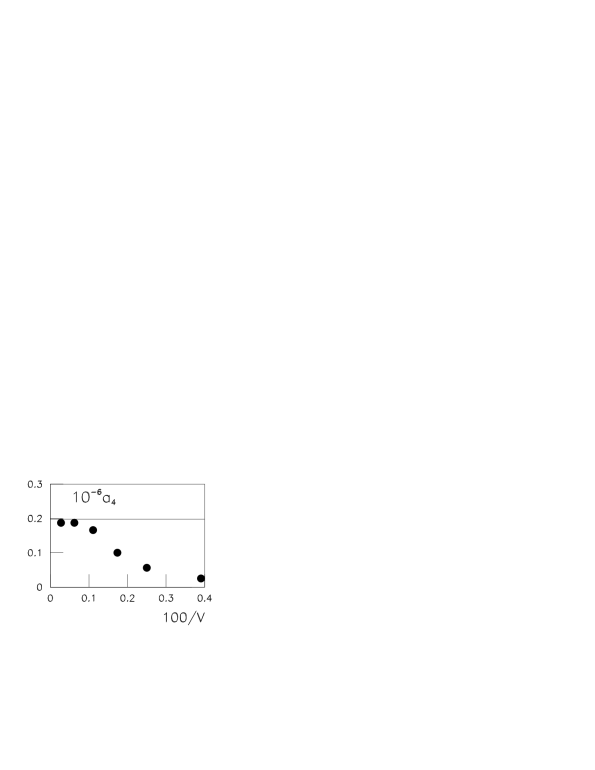
Figure 2: Normalised single-phase cumulants $a_{k}$ against $1/V$. The error bars are smaller than the size of the symbols. The horizontal lines show the values from series expansions.

The data at the larger couplings were taken on a wider range of lattice sizes. This data has been used for a direct analysis of the scaling of moments. The aim is to find the range of lattice sizes which is sufficiently large that the leading correction terms in the FSS expansion are sufficient to describe the data. The scaling of data on these lattices then allow us to extract the pure-phase susceptibility. Thus, we illustrate two different methods to extract physics from finite-size scaling at phase coexistence.

3.1 The coupling $u=0.9u_{c}$.

Figure 3: Moments $\langle m^{k}\rangle$ against $1/V$. The error bars are smaller than the size of the symbols. The curve labelled $j$ is the prediction obtained by including terms of order up to $1/V^{j}$. To avoid clutter, no more than three curves have been shown for each moment.

The first four normalized single-phase cumulants $a_{k}$ (see eq. 15) are shown in figure 2. They were obtained using the cut $m^{*}=0$, and by folding data for negative magnetisations into the interval $m\geq 0$. In the FSS theory we expect these cumulants to approach a constant. Clearly, the smallest lattices lie outside the range of validity of the theory. It is clear from the figure that $V_{k}^{(0)}$ increases with $k$. For larger $V$ the cumulants are consistent with their known asymptotic values [12] within errors. The first two cumulants can be determined with an error of less than 3% on lattices with $L/\xi>5$. This accuracy is sufficient for this measurement to be useful in the FSS analysis of moments. The rapid approach to the large volume limit is extremely useful for practical determination of the cumulants. However this also means that a numerical investigation of the neglected terms in the partition function is not feasible without much higher statistics.

The known values of $a_{k}$ [12] can be used for the scaling of the moments $m_{k}$ using the formula in eq. 7. These predictions are shown along with the data in figure 3. The previously studied $1/V$ correction corresponds to the straight line and seems to give a good approximation at large volumes. Note that the FSS theory predicts no higher term for the scaling of the second moment. The data is completely consistent with this expectation for $L/\xi$ as low as 4. Consistent with this, we found that a fit to the data on $m_{2}$ for $L/\xi\geq 4$ correctly yields the values of the first two cumulants.

The exact curves show that the fourth and higher moments definitely require terms beyond the leading $1/V$ correction for a description of the data for $L/\xi\raise 1.29167pt\hbox{$<$\kern-7.5pt\raise-4.73611pt\hbox{$\sim$}}8$. It is interesting to note that an attempt to fit a $1/V$ correction term to the data on $m_{4}$ for $L/\xi>6$ produces a good fit by a $\chi^{2}$ measure. However, the values of the first two cumulants so obtained are wrong by 7–10$\sigma$. This state of affairs is similiar to the situation reported for the two-dimensional 10-state Potts model [7].

The volume dependence of the sixth and eighth moments cannot be fitted purely by the $1/V$ term for $L/\xi\geq 6$. Note also that the exact prediction using the FSS model of eq. 7 deviates strongly from the data at increasingly larger volumes as $k$ grows.

Figure 4: The deviations $\Delta_{k}$ against $1/V$. For each moment $k$, the residue $R_{j}$ is labelled by the number $j$. To avoid clutter, only 3 of the curves are shown for $k=8$.

For a more detailed assessment of this volume dependence, we studied the difference between the predictions of eq. 7 and the measured values of the moments

$$\Delta_{k}\,=\,m_{k}({\rm meas})-m_{k}({\rm pred})\,.$$ (19)

These values are plotted in figure 4 as a function of $1/V$. Also plotted are the values of the residues

$$R_{j}^{(k)}\;=\;\sum_{i=j}^{k-1}{A_{k,i}(0)\over V^{i}}\,.$$ (20)

When analysing FSS for $m_{k}$ in terms of a series truncated at the $1/V^{j}$ term, these residues are the sum of the neglected terms. It is clear that at small volumes correction terms beyond $1/V$ are quite important.

Another striking feature that emerges is that, as $V$ decreases, there seems to be a fairly abrupt threshold at which the agreement between the $\Delta_{k}$ and the residues disappears. This threshold volume increases with $k$, and is a little larger than $V_{k}$. The data seems to indicate that the FSS theory of moments is valid for volumes $V>V_{k}^{(0)}$. The limit $V_{k}$ is less stringent for this case.

That there is a lower limit to the volumes for which the FSS theory is applicable is also shown in figure 5. Here we plot $\ln|\Delta_{k}|$ against $L$. For $L/\xi\sim 3$, it turns out that the measured values of the higher moments are much smaller than the value predicted by the series in eq. 7. As a result $\ln|\Delta_{k}|$ is large in this region. Since the highest term in the FSS series tends to dominate at small volumes, for very small $L$ we should see the trivial behaviour $\ln|\Delta_{k}|\sim(k-1)d\ln L$. At much larger values of $L/\xi$, $m_{k}$ should have a good description in terms of the FSS series. In this region we expect small values of $\Delta_{k}$, going to zero roughly as $\ln|\Delta_{k}|\sim(d-1)L$. The data for $k=10$ clearly exhibits a cross-over from a regime of large $\Delta_{k}$ to small values; the latter being reached only on the two largest lattices. In this region, the data is too noisy to characterise the approach to zero, and hence the nature of the neglected error terms.

Figure 5: The deviations $\Delta_{k}$ for $k=2$ (circles), 6 (squares) and 10 (triangles), plotted against $L$.

3.2 Other couplings.

The leading terms of the FSS theory at $h=0$ for the scaling of moments are

$$m_{2k}\;=\;m_{0}^{2k}+{\alpha_{k}\over V}+{\beta_{k}\over V^{2}}+{\gamma_{k}\over V^{3}},$$ (21)

where eq. 7 contains expressions for $\alpha_{k}$ and $\beta_{k}$ in terms of the cumulants. The coefficient $\alpha_{k}$ is related to the pure phase susceptibility, $\chi$, and the spontaneous magnetisation, $m_{0}$, by the relation

$$\alpha_{k}\;=\;(2k-1)km_{0}^{2k-2}{\chi\over\beta}.$$ (22)

Thus, for sufficiently large volumes, analysis of different moments should yield consistent values of $m_{0}$ and $\chi$. At the coupling $\beta=0.475$, we have data on lattices with $4.3\leq L/\xi\leq 34.3$. For lattice sizes which are not too large, we find that it is possible to describe the data fairly well using only the four terms shown in eq. 21. In figure 6 we show fits to the first four even moments of the magnetisation for $L/\xi\geq 10$. At the two remaining couplings, data for lattices of size $L/\xi\geq 10$ are also very well described by the same number of terms.

Figure 6: The moments $m_{2k}$ at $\beta=0.475$, for $1\leq k\leq 4$, plotted against $1/L^{2}$. The curves show the best fits to the forms described in the text. The open circles indicate the data to which these fits have been made.

Table 2: The spontaneous magentisation extracted from fits to $m_{2k}$ at the couplings shown. The errors on the final digit are indicated by the numbers in brackets.

$\beta$	$k=1$	$k=2$	$k=3$	$k=4$
$0.4750$	$0.86583(2)$	$0.86581(3)$	$0.86581(3)$	$0.8657(3)$
$0.5000$	$0.91135(2)$	$0.91135(2)$	$0.91135(2)$	$0.91136(2)$
$0.5500$	$0.95395(3)$	$0.95400(4)$	$0.95400(4)$	$0.95400(4)$

These fits yield independent estimates of $m_{0}$ from the extrapolated infinite volume value of each moment. These values, extracted from the first four even moments at three different couplings, are given in Table 2. They are completely consistent with the known exact results listed in Table 1, and with each other. Note that equally good values for $m_{0}$ can be obtained by using only the first two terms of eq. 21 to describe the data on lattices with $L/\xi\geq 15$.

The same fits allow for a second check of consistency. If we denote by $\chi^{(k)}$ the value of the pure-phase susceptibility extracted from fits to the data on $m_{2k}$, and by $m_{0}^{(k)}$ that of the spontaneous magnetisation, then this gives a prediction for the coefficient

$$\alpha_{l}^{(k)}\;=\;(2k-1)k(m_{0}^{(k)})^{2k-2}{\chi^{(k)}\over\beta}.$$ (23)

Consistency demands that for any $l$, the predicted values of $\alpha_{l}^{(k)}$ (all $k$) should be consistent within errors with the value of $\alpha_{l}$ obtained by a direct fit to the data. That this is true is shown by the values listed in Table 3.

Figure 7: The pure phase susceptibility $\overline{\chi}$ at three different couplings, extracted from FSS of data on the moments of the magnetisation. The lines are obtained from series expansions as explained in the text.

This check indicates that the data requires the retention of terms beyond $1/V$ even for lattice sizes as large as $L/\xi=15$ or more. In an attempt to analyse these large lattices with only the first two terms in eq. 21, we found that the values of $\alpha_{l}^{(k)}$ for each $l$ systematically decreased with increasing $k$. This is consistent with the fact that the next coefficient, $\beta_{k}$, is negative. This effect was not very strong; at the $3\sigma$ level there was no systematic effect. Clearly, with half as much data, we would have seen no effect. Inclusion of the $1/V^{2}$ term in the analysis reversed the trend; again the effect was weak, and could be neglected at the $3\sigma$ level. The inclusion of the $1/V^{4}$ term removed all trends within errors. This also increased the stability of the value of $\chi$ extracted from $\alpha_{k}$.

Table 3: Tests of the consistency of the first order FSS fits for $\beta=0.475$. The values of $\alpha_{l}^{(k)}$ are listed. The errors are obtained using the full covariance matrix of the fitted parameters. The diagonal entries, $\alpha_{l}$, are from direct fits to $m_{2l}$.

$k$	$l=1$	$l=2$	$l=3$	$l=4$
$1$	$2.1(1)$
$2$	$9.3(5)$	$9.9(6)$
$3$	$17(1)$	$19(1)$	$18.3(7)$
$4$	$24(1)$	$26(2)$	$26(1)$	26.9(9)

This consistency allows us to extract a stable and unique value for $\chi$ from each set of data. These are shown in figure 7. We have also estimated the pure phase susceptibilities using a low-temperature expansion to order 9 in $u$ [13]. This is sufficient for couplings at which the correlation length is less than 3. For the smaller couplings this series is extrapolated using standard techniques [14]. The results obtained from the FSS measurements are consistent with the series results.

3.3 Approach to criticality.

We have seen that the asymptotic size dependence at a fixed temperature is well described by the FSS theory for a first-order phase transition. If this temperature is near the critical end point, then we would at the same time expect FSS theory for a second-order phase transition to apply. In Section 2, we saw that these requirements are consistent. The formula for the $k$th moment, as obtained from FSS for a first-order phase transition, can, in the vicinity of $\beta_{c}$, be written in the form

$${m_{k}(\beta,h=0,L)\over m_{o}^{k}}\,=\,1+f(L/\xi)\ ,$$ (24)

where the finite-size correction $f$ depends only on the ratio $L/\xi$. In figure 8 we have plotted the fourth moment against $(\xi/L)^{2}$ for two different temperatures. Eq. 24 implies that two data sets should fall on a common curve. The figure confirms that the temperature dependence to a good approximation is described by eq. 24.

Figure 8: The fourth moment of the magnetisation at two different temperetaures, $u/u_{c}=0.9$ (filled circles) and $2\beta=0.95$ (open circles).

4 CONCLUSIONS

A finite-size scaling theory at phase coexistence, based on a formal expansion of the free energy density in terms of an external field or coupling, gives a very good description of observations when the system size $L$ is large enough. Data taken in the low-temperature phase of the Ising model indicates that the scaling of lower moments of the magnetisation for $L/\xi\raise 1.29167pt\hbox{$>$\kern-7.5pt\raise-4.73611pt\hbox{$\sim$}}6$ is completely consistent with the theory, once all terms in the expansion have been taken into account. The second moment seems to be completely consistent with the theory for lattice sizes as small as $3\xi$. Higher order moments generally require larger volumes for the theory to be applicable. Several correction terms seem to be necessary even for lattices as large as $L/\xi\geq 15$.

The relative importance of the higher correction terms is, of course, dependent on the actual values of $a_{k}$, and hence on the Hamiltonian studied. For the Ising model, these cumulants decrease with increasing $\beta$. Thus, when the temperature is small enough, and $\xi$ is smaller than one lattice spacing, the correction term of order $1/V$ suffices even for rather small $V$. This is also true for two dimensional Potts models with sufficiently large number of states.

In the numerical study of a phase transistion a first task is to determine the order of the transition. As is well known, this can be done, for example, by examining the size dependence of the susceptibility or specific heat. A linear divergence of the response function with increasing volume signals the first-order nature of the phase transition. Clearly, this requires a FSS study, but it should be noticed one is here investigating a leading-order effect. The actual usefulness of the full FSS theory in this context is therefore not obvious [9].

Having established the first-order nature of a phase transition, the primary physical quantities are cumulants, i.e., derivatives of the free-energy, for the coexisting phases. These quantities represent higher order effects in the system size. It is an important feature of the FSS theory that the finite-size corrections to these cumulants are predicted to be exponentially small. This suggests a direct measurement of them. For this purpose we have tested the method of pure-phase cuts. We found that the (lower) cumulants can be obtained in this way with reasonable accuracy on small volume systems ($8\leq L/\xi\leq 12$). Indeed, we have seen a rapid approach to the infinite volume results.

A further role of the FSS theory is to provide the possibility to perform important consistency checks. Once the cumulants are known, the FSS theory predicts the behaviour of the moments, which can be easily tested. Alternatively, when good data on intermediate volumes ($10\leq L/\xi\leq 30$) are available, then direct FSS fits can be used to extract the cumulants and thus obtain independent estimates of these. Our experience suggests that the direct extraction through single-phase cuts is the easier of the two methods.

We have shown how the FSS theory for coexisting phases goes over smoothly into the standard FSS theory for a critical system. We note further that the expansion used in developing the FSS relations is an asymptotic expansion. We have worked at the infinite volume coexistence point, where the expansions terminate at a finite number of terms, and the corrections to this result are exponentially small.

Thus, we find that finite-size effects at first-order transitions can be effectively studied in terms of scaled cumulants. These are easily extracted from data and have no size-dependence within the context of the scaling theory. As a result, their study very simply determines the limits of the theory, and tells us whether the systems used in their extraction are large enough for infinite volume physics to be extracted.

In the ten years that have passed since the first studies of finite-size scaling at first-order phase transitions, the computational power at the disposal of physicists has increased by three orders of magnitude. The ability to convert this power into precise knowledge of the physics contained in a Hamiltonian depends upon control of the systematics of finite-size effects. This control is now complete.

References

- [1] M. E. Fisher and A. N. Berker, Phys. Rev. B26 (1982) 2507.
- [2] K. Binder and D.P. Landau, Phys. Rev. B30 (1984) 1477.
- [3] M.S. Challa, D.P. Landau and K. Binder, Phys. Rev. B34 (1986) 1841.
- [4] C. Borgs and R. Kotecký, J. Stat. Phys. 61 (1990) 79.
- [5] C. Borgs, R. Kotecký and S. Miracle-Solé, J. Stat. Phys. 62 (1991) 529.
- [6] C. Borgs and W. Janke, Phys. Rev. Lett. 68 (1992) 1738.
- [7] A. Billoire, R. Lacaze and A. Morel, Nucl. Phys. B370 (1992) 773.
- [8] J. Lee and J.M. Kosterlitz, Phys. Rev. B43 (1990) 3265.
- [9] A. Billoire, T. Neuhaus and B. Berg, Saclay preprint SPhT-92/120, November 1992.
- [10] B. Berg and T. Neuhaus, Phys. Lett. B267 (1991) 249; Phys. Rev. Lett. 68 (1992) 9.
- [11] S.N. Isakov, Commun. Math. Phys. 95 (1984) 427.
- [12] G.A. Baker Jr and D. Kim, J. Phys. A: Math. Gen. 13 (1980) L103.
- [13] C. Domb, in Phase Transitions and Critical Phenomena, Vol. 3, Eds. C. Domb and M. S. Green, Academic Press, London, 1974.
- [14] D. S. Gaunt and A. J. Guttmann, in Phase Transitions and Critical Phenomena, Vol. 3, Eds. C. Domb and M. S. Green, Academic Press, London, 1974.