Abstract

We present results for the confinement-deconfinement interface tension $\sigma_{cd}$ of quenched QCD. They were obtained by applying Binder’s histogram method to lattices of size $L^{2}\times L_{z}\times L_{t}$ for $L_{t}=2$ and $L=8,10,12\mbox{ and }14$ and various $L_{z}\in[L,\,4\,L]$. The use of a multicanonical algorithm and rectangular geometries have turned out to be crucial for the numerical studies. We also give an estimate for $\sigma_{cd}$ at $L_{t}=4$ using published data.

1 Introduction

At high temperatures the structure of strongly interacting particles is supposed to be quite different from its low temperature form. The familiar hadron spectrum will be dissolved and quarks and gluons will become the fundamental degrees of freedom (“quark gluon plasma”). These two phases are probably separated by a first order phase transition at a critical temperature $T_{c}\approx 100-200\,\mbox{ MeV }$ (see [1, 2, 3, 4]). The existence of this transition might have interesting consequences for the nucleosynthesis in the early universe. One possible scenario which could happen when the temperature of the universe is cooled down below $T_{c}$ is the following [5, 6, 7]: First the universe got slightly supercooled because of the extra interfacial free energy which is required for the generation of regions of hadronic phase within the quark gluon plasma. When this so called ”nucleation” occurred, the universe was reheated to $T_{c}$ because of the gain in latent heat. Then the generated hadronic bubbles growed keeping the temperature constant until they finally met. The situation was now reversed: There were bubbles of quark gluon plasma within the hadronic phase. The temperature could not be maintained any more by the gain of latent heat und was thus decreased so that also the remaining bubbles hadronized. Since the baryonic density in the quark gluon plasma may be much higher than in the hadronic phase [8], an inhomogeneous baryon number distribution resulted from this condensation process. If the scale of these inhomogeneities is between the diffusion length that protons moved until nucleosynthesis set in and the one of the neutrons, the baryon number inhomogeniety transformed into an inhomogeneity of the neutron to proton ratio. This obviously has consequences for the element synthesis [7, 8].

In the early stage of this development an important new length scale shows up: The average distance $R_{i}$ between the hadronic bubbles after the universe had been reheated to $T_{c}$. Assuming that this point was reached when the shock waves emitted from the hadronic bubbles met, this distance has been calculated to be [5, 6, 9]

$$R_{i}=7\cdot 10^{5}\,\frac{(\sigma/T_{c}^{2})^{3/2}}{(L/T_{c}^{4})\,T_{c}^{2}[\mbox{MeV}^{2}]}$$ (1.1)

where L is the latent heat of the transition and

$$\sigma_{cd}=\frac{F}{A\,T_{c}}$$ (1.2)

is the reduced interface tension of an interface between the hadronic (“confined”) and the quark gluon plasma (“deconfined”) phase. $A$ is the area of this interface, and $F$ is its free energy. Thus the knowledge of the values of $\sigma_{cd}$ and $L$ would give the scale for the inhomogeneities in the baryon number which has been generated by the deconfinement phase transition. In order to obtain inhomogeneities which are not washed out by the diffusion of the protons, $R_{i}$ should be at least of the order of 0.5m [9].

The latent heat has been measured in e. g. [4]. The interface tension has been determined numerically at the critical temperature $T_{c}=1/L_{t}$ where $L_{t}$ is the lattice extent in the euclidean time direction. Essentially two different types of methods have been used. In the first type coexistence of the confined and the deconfined phase was enforced by keeping different parts of the lattice at different temperatures or by applying an external field. This breaks translation invariance and pins the interface at a certain position. The properties of a pinned interface will in general be different from the ones of the free interface one is interested in. To extract the interface tension one should first perform the infinite volume limit and then turn off the temperature gradient or the external field. In practice this is difficult because in a numerical simulation the lattice size is necessarily limited. This causes finite size effects which must be understood before one can extrapolate results reliably to the infinite volume limit. Using this type of methods for $L_{t}=2$ the Boston group obtained $\sigma_{cd}=0.12(2)T_{c}^{2}$ [10] while the Helsinki group quotes $\sigma_{cd}=0.08(2)T_{c}^{2}$ [11]. Closer to the continuum limit for $L_{t}=4$ the Boston group quotes $\sigma_{cd}=0.027(4)T_{c}^{2}$ [12]. But the validity of this method has been questioned lately by the authors of refs. [13, 14]. Using the same method as in ref. [12] for the two-dimensional seven-states Potts model one finds numerical values which are in disagreement with an analytic result (see ref. [15]).

The second type of calculations is done without any pinning of the interface. One approach of this kind makes use of the finite volume splitting of the spatial transfer matrix spectrum. For $L_{t}=2$ one obtains $\sigma_{cd}=0.139(4)\,T_{c}^{2}$ [16]. In order to apply this method, the extension of the lattice in one spatial direction ($L_{z}$, say) has to be much larger than the corresponding tunneling correlation length $\xi_{t}$. Since the latter increases exponentially with the area $A$ of the interface one is restricted to rather small interface areas. In contrast to this for the modified version of Binder’s histogram method [17] which we are using in this work one has to use lattices of extension $\xi_{b}\ll L_{z}\ll\xi_{t}$ where $\xi_{b}$ is the bulk correlation length.

In this paper we apply Binder’s histogram method to rectangular lattices ($L_{z}>L$). We demonstrate how this eliminates the interfacial interactions which had complicated previous studies. We give a simple consistency criterion for the absence of such interactions and show that our data are well described by a capillary wave model. This reduces the number of fitting parameters to two (one of which is the interface tension). We obtain $\sigma_{cd}=0.103(7)\,T_{c}^{2}$ which is consistent with the older data but slightly lower than the more accurate determination by the transfer matrix method. We will argue that this might be due to the rather small interfaces used for the transfer matrix method.

Our method is described in section 2. For the numerical work it was essential to use a multicanonical algorithm for quenched $QCD$ [18]. This is described in section 3. In section 4 we give our numerical results for the tunneling autocorrelation times, the critical coupling $\beta_{c}$ and the interfacial free energy. Finally we give our conclusions in section 5.

2 The Interfacial Free Energy

We consider SU(3) pure gauge theory with the Wilson action $S$ on rectangular lattices of size $L^{2}\times L_{z}\times L_{t}$ and $L_{z}$ varying between $L$ and $4L$ at the critical coupling $\beta_{c}$ for $L_{t}=2$. We use periodic boundary conditions in the time direction and $C-$periodic boundary conditions [19] in the spatial directions, i.e.

$$U_{\mu}(\vec{x}+L_{i}\vec{e}_{i},t) = U_{\mu}^{*}(\vec{x},t),\mbox{ for }i=x,y,z$$ (2.1)

$$U_{\mu}(\vec{x},t+L_{t}) = U_{\mu}(\vec{x},t).$$ (2.2)

The value of the Polyakov line $\Omega_{L}(\vec{x})\equiv tr\left(\prod_{t=1}^{L_{t}}U_{0}(\vec{x},t)\right)$ satisfies

$$\Omega_{L}(\vec{x}+L_{i}\vec{e}_{i})=\Omega_{L}^{*}(\vec{x})\mbox{ for }i=x,y,z$$ (2.3)

because of the $C-$periodic boundary conditions. Therefore, no bulk configurations in either of the two deconfined phases that have nonvanishing imaginary part of $\Omega_{L}\equiv 1/(L^{2}L_{z})\sum_{\vec{x}}\Omega_{L}(\vec{x})$ can exist and the probability distribution $P_{L}(\rho)d\rho$ of $\rho\equiv Re\,\Omega_{L}$ takes the form sketched in Fig.2.

Figure 1: Schematic probability distribution for the order parameter. The dotted line indicates the multicanonical distribution.

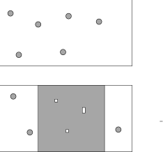
Figure 2: Typical cuts through the lattice in the $y-z-$plane at values $\rho^{(1)}$ (first picture) and $\rho^{(min)}$ (second picture) of the order parameter. The two phases are represented by white resp. shaded areas.

The system is most likely in either the confined phase at $\rho^{(1)}$ or the one remaining deconfined phase corresponding to $\rho^{(2)}$. When $\rho$ is increased from $\rho^{(1)}$, bubbles of deconfined phase form. These configurations are suppressed by the interfacial free energy $\sigma_{cd}A$, where $A$ is the surface area of the bubble. The largest bubble grows until finally $A$ is larger than the area $L^{2}$ of two planar interfaces which devide the lattice into three parts as depicted in the second part of Fig. 2. Since the interface area of the two planar interfaces is independent of $\rho$ the probability $P_{L}$ is constant in the region where their contributions dominate, i.e. around $\rho^{(min)}$. Because of the $C-$periodic boundary conditions these interfaces always separate a region in the confined phase from one in the deconfined phase that has $Im(\Omega_{L})=0$. Thus the corresponding configurations will be exponentially suppressed by the interfacial free energy of two confined-deconfined interfaces.

In addition there will be internal fluctuations of the interfaces. These fluctuations may be described by a simple capillary wave model (see [20]). There one assumes that the interfaces are almost flat, i.e. fluctuations are small. The energy is proportional to the area of the interface. Expanding the energy around its equilibrium position leads to a simple Gaussian model for the interface, the so called “capillary wave model”. In this model the width of an interface increases only with $\sqrt{\ln\,A}$ (see [21]). On the other hand, for configurations corresponding to the center of the histogram the two interfaces are separated by roughly $L_{z}/2$. Therefore, if one choses $L_{z}\geq L$, the overlap of the two interfaces for $C$-periodic boundary conditions should be negligible for $L$ large enough. However, it turns out that compared to cubic lattices the choice $L_{z}>L$ will reduce the interactions, especially for smaller systems. Still, one should not be in the region $L_{z}\gg\xi_{t}$ where $\xi_{t}$ is the tunneling correlation length [16, 22, 23]. For two independent interfaces one gets [24]

$$P_{L}^{int}\propto L_{z}^{2}\cdot L^{d-3}\cdot\exp\left(-2\sigma_{cd}L^{d-1}\right).$$ (2.4)

for $d-$dimensional spatial volumes. It was shown in [25] for $d=2$ that the constraint $\rho=\rho^{(min)}$ does not change this result.

In order to extract $P_{L}^{int}$ from the total probability distribution $P_{L}(\rho)\,d\rho$ we make an ansatz analogous to the one used in ref. [26]: We assume that the total probability distribution for a system of volume $V=L^{2}\times L_{z}$ is given by the sum of two Gaussians

$$P_{L}^{(i)}(\rho)=\sqrt{\frac{V}{2\pi\chi_{i}}}\cdot\exp\left(-\frac{V}{2\chi_{i}}(\rho-\rho^{(i)})^{2}\right),\,i=1,2,$$ (2.5)

and the interface contribution by eq. (2.4) so that

$$P_{L}(\rho)\propto P_{1}\,P_{L}^{(1)}(\rho)+P_{2}\,P_{L}^{(2)}(\rho)+P_{3}\,P_{L}^{int}$$ (2.6)

where $P_{1},\,P_{2}$ and $P_{3}$ are the relative weights of the two bulk phases and the interface configurations. In [27] it was shown that

$$P_{1}=\frac{\exp(-\beta Vf_{1}(\beta,j))}{\exp(-\beta Vf_{1}(\beta,j))+q\exp(-\beta Vf_{2}(\beta,j))}$$

and

$$P_{2}=\frac{q\exp(-\beta Vf_{2}(\beta,j))}{\exp(-\beta Vf_{1}(\beta,j))+q\exp(-\beta Vf_{2}(\beta,j))}$$ (2.7)

for a $q-$states Potts model. Here $f_{1}$ and $f_{2}$ are the free energy densities of the two phases. In appendix A we will derive corresponding finite size scaling formulas for the Polyakov line and its susceptibility as well as for some finite volume estimates of the critical coupling $\beta_{c}$. We will use these results as a consistency check for this ansatz and in order to determine $\beta_{c}$.

By analogy we conclude that

$$P_{3}=\frac{\exp(-\beta(V_{1}f_{1}+V_{2}f_{2}))}{\exp(-\beta Vf_{1})+q\exp(-\beta Vf_{2})}$$ (2.8)

for the relative weight of a configuration in which two interfaces separate regions of volume $V_{1}$ and $V_{2}$ in either of the bulk phases from each other. Since at the minimum $\rho^{min}$ one has $V_{1}\approx V_{2}\approx V/2$, the dependence on $f_{i}$ will cancel in the combination

$$\frac{\overline{P_{L}}^{max}}{P_{L}^{min}}\equiv\frac{\sqrt{P_{L}^{max,1}\,P_{L}^{max,2}}}{P_{L}^{min}}$$ (2.9)

of the minimal probability $P_{L}^{min}\propto P_{3}\,P_{L}^{int}$ and the maxima $P_{L}^{max,i},\,i=1,2$. This ratio is therefore only weakly dependent on $\beta$. In contrast to this, in $P_{L}^{min}\propto P_{3}\cdot P_{L}^{int}$ the volume dependence of $P_{3}$ will only cancel when $f_{1}=f_{2}$, which introduces a fine tuning problem for $\beta$. In addition, the overall normalization of $P_{L}(\rho)$ is needed for $P_{L}^{min}$, but not for the combination (2.9). Thus the latter is our preferred quantity for the analysis of our numerical data. In order to cancel the preexponential factors we define

$$F_{L}^{(1)}\equiv\frac{1}{2L^{2}}\ln\frac{\overline{P_{L}}^{max}}{P_{L}^{min}}+\frac{3}{4}\frac{\ln L_{z}}{L^{2}}-\frac{1}{2}\frac{\ln L}{L^{2}}.$$ (2.10)

This approaches asymptotically

$$F_{L}^{(1)}\rightarrow\sigma_{cd}+\frac{b_{1}}{L^{2}}\vspace{1cm}\mbox{ for }L_{z}\geq L\rightarrow\infty$$ (2.11)

while

$$F_{L}^{(2)} \equiv -\frac{1}{2L^{2}}\ln P_{L}^{min}+\frac{\ln L_{z}}{L^{2}}$$ (2.12)

$$\rightarrow \sigma_{cd}+\frac{b_{2}}{L^{2}}\vspace{1cm}\mbox{ for }L_{z}\geq L\rightarrow\infty$$ (2.13)

In order to calculate the probability distribution $P_{L}(\rho)$, one has to simulate the SU(3) pure gauge theory at the deconfinement phase transition. But because of eq. (2.4) any standard local updating algorithm will have autocorrelation times $\tau_{L}$ which increase exponentially with $L^{2}$ (”supercritical slowing down”). The use of the multicanonical algorithm [28, 29, 30, 31] reduces this effect considerably.

3 The Multicanonical Algorithm

Monte Carlo simulations with a local Metropolis or heat bath algorithm suffer from supercritical slowing down close to first order phase transitions , i.e. the tunneling time $\tau_{L}$ for a system of volume $V=L^{2}\times L_{z}$ is expected to be proportional to the inverse of the probability of a system with interfaces (actually there will be two interfaces because of the boundary conditions),

$$\tau_{L}\propto V^{z}\cdot P_{L}^{min}\approx V^{z}\exp(2L^{2}\sigma_{cd}),\vspace{0.5cm}$$ (3.1)

with an unknown exponent $z$, and therefore diverges exponentially with the area $A=L^{2}$ of an interface.

In order to overcome this problem, the multicanonical algorithm does not sample the configurations with the canonical Boltzmann weight

$${\cal P}_{L}^{can}(S)\propto\exp(\beta S),$$ (3.2)

where $S=1/3\,\sum_{\Box}\,tr\,U_{\Box}$ is the Wilson action in four dimensions, but rather with a modified weight

$${\cal P}_{L}^{mc}(S)\propto\exp(\beta_{L}(S)S+\alpha_{L}(S)).$$ (3.3)

The coefficients $\alpha_{L}$ and $\beta_{L}$ are chosen such that the probability $P_{L}$ (not to be confused with the Boltzmann weights) is increased for all values of the action in between the two maxima $\rho^{(1)}\mapsto S_{L}^{max,1}$ and $\rho^{(2)}\mapsto S_{L}^{max,2}$ , as shown schematically in Fig. 2 (where $\rho$ is identified with the action here). Finally data are analyzed from the multicanonical samples by reweighting with $\exp((\beta-\beta_{L}(S))S-\alpha_{L}(S))$.

In order to approximate the weights ${\cal P}_{L}^{mc}$ leading to the distribution $P_{L}^{mc}$ of Fig. 2, we start from some good estimate of the canonical distribution $P_{L}$ (see below) at the coupling $\beta_{P}(L)$ which corresponds to equal weight in both phases. This will lead to different heights of the two peaks. Then we take a partition

$$S_{L}^{0}=-6VL_{t} < S_{L}^{1}\equiv S_{L}^{max,1}<S_{L}^{2}<\ldots<S_{L}^{N/2}\equiv S_{L}^{min}<\ldots$$ (3.4)

$$\ldots <S_{L}^{N-1}\equiv S_{L}^{max,2}<S_{L}^{N}=6VL_{t}$$

of the interval $-6VL_{t}\leq S\leq 6VL_{t}$. The coefficients $\alpha_{L}$ and $\beta_{L}$ are chosen to be constants $\alpha_{L}^{k}$ and $\beta_{L}^{k}$ in the intervals $[S_{L}^{k},S_{L}^{k+1})$ such that $\ln P_{L}^{mc}$ interpolates the linear function

$$\ln P_{L}^{max,1}+(\ln P_{L}^{max,2}-\ln P_{L}^{max,1})\cdot\frac{S-S_{L}^{max,1}}{S_{L}^{max,2}-S_{L}^{max,1}}.$$ (3.5)

continuously between the points $S_{L}^{k}$ and $S_{L}^{k+1}$ for $k=1$ to $N-2$. The Boltzmann weight is identical to the canonical one in the first and last interval. We arrive at

$$\beta_{L}^{k}-\beta=\left\{\begin{array}[]{ll}0&,k=0\\ \delta\beta+\ln\left(\frac{P_{L}(S_{L}^{k})}{P_{L}(S_{L}^{k+1})}\right)/(S_{L}^{k+1}-S_{L}^{k})&,k=1,\ldots,N-2\\ 0&,k=N-1\end{array}\right.$$ (3.6)

where $\delta\beta\equiv\ln\left(\frac{P_{L}^{max,2}}{P_{L}^{max,1}}\right)/(S_{L}^{max,2}-S_{L}^{max,1})$, and the $\alpha_{L}^{k}$ are given by

$$\alpha_{L}^{k+1}\equiv\alpha_{L}^{k}+(\beta_{L}^{k}-\beta_{L}^{k+1})S_{L}^{k+1},\;\alpha_{L}^{0}=\delta\beta\cdot S_{L}^{max,1}.$$ (3.7)

The partition $\{S_{L}^{k}\}$ which is in principle arbitrary is defined by demanding

$$\frac{P_{L}(S_{L}^{k+1})}{P_{L}(S_{L}^{k})}=\left\{\begin{array}[]{ll}1/r_{1}&,k=1,\ldots,N/2-1\\ r_{2}&,k=N/2,\ldots,N-2,\end{array}\right.\hfill(2.8)$$ (3.10)

such that $r_{1}^{N/2-1}=P_{L}^{max,1}/P_{L}^{min}$ and $r_{2}^{N/2-1}=P_{L}^{max,2}/P_{L}^{min}$. This generalizes the formulas given in [28, 29] to the case $P_{L}^{max,1}\neq P_{L}^{max,2}$ by introducing a $\delta\beta\neq 0$. In addition the specific choice for $r_{1}$ and $r_{2}$ assures that the probability of $S_{L}^{min}$ is lifted by the correct amount.

We apply this algorithm to the $SU(3)$ pure gauge theory at the deconfinement phase transition. The multicanonical data sampling was done with a 5-hit Metropolis algorithm as well as with a Creutz heat bath algorithm modified according to eq. (3.3). In both cases three independent $SU(2)$-subgroups are updated following the idea of ref. [32]. The modifications needed for the Metroplis algorithms are straightforward. Because of the dependence of $\alpha_{L}$ and $\beta_{L}$ on the total action $S$, the update of the active link has to be done in scalar mode. However, most of the computation time is needed for the calculation of the staples surrounding the active link, and this is still vectorizable.

The modifications for the Creutz algorithm are more complicated. The reason is that one has to know the action for the updated configuration already for the proposal of the link. Therefore, whenever it is possible to cross one of the interval boundaries (e.g. $S_{L}^{k}$) of the multicanonical action, one first has to calculate the probabilities $P_{k-1}$ and $P_{k}$ that the new action will be below or above the interval boundary.

For simplicity we will describe the modifications for an SU(2) gauge group. The imbedding in the full SU(3) group is done according to [32]. We adapt the standard notation for the subgroup update (see e.g. [33]). Let $h$ be the ‘active’ link, $\Sigma=\xi u,\,u\in SU(2),$ the sum of the surrounding staples, and $a=uh=a_{0}\cdot 1+\vec{a}\cdot\vec{\sigma}$. Let finally $b$ represent all other links. Then one wants to generate a new link $a_{0}$ with the weight

$${\cal P}(a_{0},b)={\cal N}^{-1}\,\sqrt{1-a_{0}^{2}}\,\exp\left(\alpha(S)+\beta(S)S(a_{0},b)\right)d\,a_{0},\vspace{0.5cm}-1\leq a_{0}\leq 1.$$ (3.11)

Now $S(a_{0},b)$ depends on $a_{0}$ only through the combination $s(a_{0},\xi)=\frac{2}{3}\xi a_{0}$. It is convenient to define $\tilde{S}(a_{0},b)\equiv S(a_{0},b)-s(a_{0},\xi)$. If $|\tilde{S}-S_{L}^{k}|>\frac{2}{3}\xi$ for all $k$, no interval boundary can be crossed due to the update of $a_{0}$, and one can proceed in the standard way. If on the other hand $|\tilde{S}-S_{L}^{k}|\leq\frac{2}{3}\xi$ for one k, the total action $S$ might cross the interval boundary $S_{L}^{k}$ by the update of $a_{0}$. Then the selection of $a_{0}$ according to

$${\cal P}_{1}(a_{0},b)={\cal N}_{1}^{-1}\,\exp(\alpha(S)+\beta(S)S(a_{0},b))d\,a_{0},\vspace{0.5cm}-1\leq a_{0}\leq 1.$$ (3.12)

has to be done in two steps. First one has to select the interval in which the action will be after the update, and then to select $a_{0}$ from the corresponding interval. Let us assume that the intervals are large enough so that one can only enter the intervals $[S_{L}^{k-1},S_{L}^{k})$ and $[S_{L}^{k},S_{L}^{k+1})$. For $SU(3)$ in four dimensions this means that the length of each interval must be larger than eight which in practice is not a very strong restriction. The ratio $r=P_{k}/P_{k-1}$ of the probabilities to end up in either of the two intervals is given by

$$r = \frac{\int_{I_{k-1}}\exp\left(\alpha_{k-1}+\beta_{k-1}S(a_{0},b)\right)}{\int_{I_{k}}\exp\left(\alpha_{k}+\beta_{k}S(a_{0},b)\right)}$$

$$= \frac{\beta_{k-1}}{\beta_{k}}\cdot\frac{\exp\left(-\beta_{k}\left(S_{L}^{k}-\tilde{S}(a_{0},b)-\frac{2}{3}\xi\right)\right)-1}{1-\exp\left(-\beta_{k-1}\left(S_{L}^{k}-\tilde{S}(a_{0},b)+\frac{2}{3}\xi\right)\right)}.$$

Here $I_{k-1}\equiv[-1,3(S_{L}^{k}-\tilde{S}(a_{0},b))/(2\xi)]$ and $I_{k}\equiv[3(S_{L}^{k}-\tilde{S}(a_{0},b))/(2\xi),1]$. Because of the assumption $P_{k-1}+P_{k}=1$ one gets

$$P_{k-1}=\frac{1}{1+r},\vspace{0.5cm}\mbox{ and }P_{k}=1-P_{k-1}.$$ (3.14)

Having chosen the interval with this probability, the selection of $a_{0}$ is done again in the standard way by taking

$$a_{0}=1+\frac{\log x}{\frac{2}{3}\xi}$$ (3.15)

where $x$ is distributed uniformly such that $a_{0}$ is in the chosen interval. In a final step one uses an accept/reject procedure to fix up the factor $\sqrt{1-a_{0}^{2}}$.

It is clear that this step cannot be vectorized since the change of any of the links $b$ might change the couplings $\alpha_{L}^{k}$ and $\beta_{L}^{k}$ which are to be taken for the heat bath step for $a_{0}$. But in a practical application the total action will hardly ever cross an interval boundary so that one can allways try to do a number of link updates with the usual, vectorizable Creutz heat-bath update. One just has to check afterwards whether in any of these steps one has crossed an interval boundary. The worst which can happen is that one has to repeat a few update steps, but as mentioned, this will occur only rarely. In [18] we have demonstrated the efficiency of the multicanonical algorithm for SU(3) pure gauge theory and have shown that one can indeed achieve a vector speed which is comparable to the canonical Creutz heat bath algorithm.

We apply the algorithm to the determination of the interfacial free energy.

4 Numerical Results

4.1 Fighting the supercritical slowing down

We simulate systems of size $L^{2}\times L_{z}\times 2$ at Wilson couplings $\beta_{sim}$ close to the deconfinement phase transition. We use a multicanonical Creutz heat bath algorithm with $N$ interpolating intervals for the multicanonical action. Each heat bath step was followed by 4 overrelaxation steps. We define the tunneling autocorrelation time $\tau_{L}$ by the exponential decay of the autocorrelation function

$$A(t) = B(t)/B(0),$$

$$B(t) = \mbox{$\langle C(k,t)\rangle$}_{k=1}^{M-t}$$

$$C(k,t) = (O(k+t)-\mbox{$\langle O(i+t)\rangle$}_{i=1}^{M-t})(O(k)-\mbox{$\langle O(i)\rangle$}_{i=1}^{M-t})$$ (4.1)

with $\mbox{$\langle O(i)\rangle$}_{i=1}^{m}:=\sum_{i=1}^{m}O(i)/m$ of the total action $S$. The autocorrelation time $\tau_{L}$ is listed in table 1 together with other simulation parameters. The numbers $\tau_{L}$ obtained from $Re(\Omega_{L})$ are consistent with this.

$\begin{array}[]{|c|c|c|c|c|c|c|c|}\hline\cr L^{2}\times L_{z}&V&\beta_{sim}&N&N_{upd}&\tau_{L}&1/P_{L}^{min}&\overline{P_{L}^{max}}/P_{L}^{min}\\ \hline\cr\hline\cr 8^{2}\times 8&512.00&5.0940&14&56000&110(10)&2.1(3)&11(1)\\ \hline\cr 8^{2}\times 16&1024.0&5.0947&14&75000&170(10)&3.3(2)&19(1)\\ \hline\cr 8^{2}\times 24&1536.0&5.0947&14&75000&190(20)&1.7(3)&11(1)\\ \hline\cr 8^{2}\times 30&1920.0&5.0947&14&70000&110(10)&1.6(4)&10(1)\\ \hline\cr 10^{2}\times 10&1000.0&5.0950&14&80000&190(30)&5.9(4)&37(2)\\ \hline\cr 10^{2}\times 30&3000.0&5.0947&14&84000&500(50)&9.0(9)&81(4)\\ \hline\cr 10^{2}\times 40&4000.0&5.0944&14&88000&450(70)&5.2(5)&55(5)\\ \hline\cr 12^{2}\times 12&1728.0&5.0928&14&120000&360(60)&18.3(6)&100(15)\\ \hline\cr 12^{2}\times 36&5184.0&5.0943&14&85000&1100(120)&49(3)&652(30)\\ \hline\cr 14^{2}\times 42&8232.0&5.0943&32&115000&1300(150)&290(10)&4600(200)\\ \hline\cr\end{array}$

Table 1: The autocorrelation time $\tau_{L}$ in comparison to $P_{L}^{min}$ and $\overline{P_{L}^{max}}/P_{L}^{min}$. We did simulations with $N_{upd}$ sweeps of an overrelaxed Creutz heat bath algorithm at the Wilson coupling $\beta_{sim}$. $N$ is the number of interpolating intervals for the multicanonical action.

Since for the largest lattices we could not observe any tunnelings within reasonable simulation times using a canonical heat bath algorithm, we cannot give a quantitative comparison of the algorithms in this case. Instead, we give the inverse probability $(P_{L}^{min})^{-1}$ which is expected to govern the supercritical slowing down of a canonical algorithm. Its growth is indeed much larger than the growth of $\tau_{L}$ for the multicanonical algorithm. Note however that the parameters for the multicanonical update where not even optimized in all cases which explains the irregularities in $\tau_{L}$.

4.2 Finite size scaling

Figure 3: The Polyakov line $\rho_{L}$ and its susceptibility $\chi_{L}$ as a function of the Wilson coupling.

Figure 4: The coupling $\beta_{m}$ as a function of the volume together with a linear fit.

$\begin{array}[]{|c|c|c|c|c|}\hline\cr L^{2}\times L_{z}&\beta_{N}&\beta_{P}&\beta_{m}&\chi_{L}^{max}\cdot 100/V\\ \hline\cr\hline\cr 8^{2}\times 8&-&5.0945(5)&5.0946(40)&2.7(5)\\ \hline\cr 8^{2}\times 16&-&5.0943(2)&5.0942(20)&2.6(5)\\ \hline\cr 8^{2}\times 24&-&5.0939(2)&5.0938(20)&2.3(4)\\ \hline\cr 8^{2}\times 30&5.0945(10)&5.0945(2)&5.0946(20)&2.2(7)\\ \hline\cr 10^{2}\times 10&-&5.0949(1)&5.0948(30)&2.8(8)\\ \hline\cr 10^{2}\times 30&5.0942(10)&5.0944(1)&5.0944(10)&2.6(9)\\ \hline\cr 10^{2}\times 40&5.0939(10)&5.0943(1)&5.0944(10)&2.5(1.3)\\ \hline\cr 12^{2}\times 12&-&5.0940(3)&5.0942(30)&2.7(1.5)\\ \hline\cr 12^{2}\times 36&5.0942(8)&5.0942(1)&5.0942(8)&2.7(1.0)\\ \hline\cr 14^{2}\times 42&-&5.0943(1)&5.0942(6)&2.6(1.2)\\ \hline\cr\infty&5.0941(10)&5.0943(1)&5.0943(5)&-\\ \hline\cr\end{array}$

Table 2: The three estimates $\beta_{N},\,\beta_{m},\,$ and $\,\beta_{P}$ of the critical coupling $\beta_{c}$ together with the maximum $\chi_{L}^{max}$ of the specific heat. In the last line the infinite volume extrapolations are given.

From the simulations described above we determine the average Polyakov line $\rho_{L}$ and its susceptibility $\chi_{L}(\beta)$. The results for the largest volumes are shown in Fig. 4. As shown in the appendix A, the ansatz in eq. (2.6) leads to the following finite size behaviour: The coupling $\beta_{N}$ at which $\rho_{L}$ becomes independent of the volume should approach $\beta_{c}$ exponentially fast in $L$. The same should be true for the coupling $\beta_{P}$ for which both peaks of the probability distribution have the same weight. For our data both estimates are independent of $L$ for the five largest volumes within the statistical errors. Therefore we take the average values as infinite volume extrapolations. The difference of the location $\beta_{m}$ of the maximum of the susceptibility to $\beta_{c}$ should be proportional to $1/V^{2}$ while the leading contribution of the height of the maximum grows proportional to $V$. As can be seen from Figs. 4 and 4 and Table 2, our data are consistently described by this. For the critical coupling we extract an overall average

$$\beta_{c}=5.0943(1)$$ (4.2)

which is consistent with the result of ref. [34]. However, the volume of our largest lattice is about five times bigger than their largest one (which was $12^{3}$).

4.3 The interface tension

We determine the probability distributions for $L_{t}=2$ and the spatial volumes $L^{2}\times L_{z}$ with $L=8,\,10,\,12,\mbox{ and }14$ and $L_{z}=3L$. In addition, we vary $L_{z}$ around this point and compare to the results for cubic lattices given in [18]. Fig. 6 shows the real part of $\Omega_{L}(z)\equiv 1/L^{2}\,\sum_{x,y}\Omega_{L}(x,y,z)$ for a typical configuration close to $\rho^{(min)}$ on a $14^{2}\times 42\times 2$ lattice.

Figure 5: $Re\,\Omega_{L}(z)$ for a $14^{2}\times 42\times 2$ lattice. The dotted lines indicate the bulk expectation values.

Figure 6: Probability distributions for the real part of the Polyakov line for the largest values of $L_{z}$.

As expected from section 2, one can identify two interfaces between the confined phase and the deconfined phase. The imaginary part of $\Omega_{L}$ is always zero. In Fig. 6 the resulting probability distributions are shown. In contrast to the distributions for cubic volumes ($L=8,\,10,$ and $12$, see [18]) they all have a region of constant probability in between the two peaks. In Fig. 8 it is demonstrated for $L=10$ how a plateau forms when one increases $L_{z}$. The small increase of $P_{L}^{min}$ between $L_{z}=30$ and $40$ is due to the translational modes of the interfaces and is consistent with eq. (2.4), as is demonstrated in Fig. 8. This supports the scenario developed in section 2 for asymmetric lattices while for small cubic lattices it casts some doubt on its applicability. However, one should note that we are not (and must not be) in the region $L_{z}\gg\xi_{t}$ where $\xi_{t}$ is the tunneling correlation length [16, 22, 23]. For $L=12\mbox{ and }14$ we did not vary $L_{z}$ but took the existence of a plateau as a criterion for the validity of our assumptions.

Figure 7: Probability distributions for $L=10$.

Figure 8: The $L_{z}$-dependence of $F_{L}^{(1)}$ for $L=8\mbox{ and }10$.

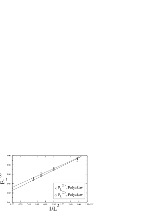
Figure 9: Results for $F_{L}^{(i)}$ together with the linear fits.

In order to extract the interface tension we evaluate the quantities $F_{L}^{(1)}$ and $F_{L}^{(2)}$. According to eqs. (2.11) and (2.13) both quantities should be linear functions of $1/L^{2}$. Their intercept with the $y$-axis is $\sigma_{cd}$. We extract $F_{L}^{(1)}$ and $F_{L}^{(2)}$ from the probability distributions of Fig. 6. The results are plotted in Fig. 9 together with the corresponding linear fits. For the interface tension we get from $F_{L}^{(1)}$ the value $\sigma_{cd}/T_{c}^{2}=0.104(7)$. As argued in section 4.3 the quantity $F_{L}^{(2)}$ is subject to a fine tuning problem. Nevertheless trying a fit results in $\sigma_{cd}/T_{c}^{2}=0.090(4)$ which is still rather close to the other value. Finally we replace the Polyakov line by the total action in all the calculations and get $\sigma_{cd}/T_{c}^{2}=0.101(6)$ for $F_{L}^{(1)}$ and $\sigma_{cd}/T_{c}^{2}=0.092(4)$ for $F_{L}^{(2)}$. Our overall result taken from $F_{L}^{(1)}$ is

$$\frac{\sigma_{cd}}{T_{c}^{2}}=0.103(7)\,\mbox{ for }L_{t}=2.$$ (4.3)

It agrees with the results in [10, 11, 12] (where the error bars are much larger) while it is smaller than the one given in [16]. This might indicate that the transverse extensions used in [16] (which are at most $8\times 8$) are too small, thereby restricting the fluctuations of the interfaces too strongly. Still the discrepancy between these results and [18, 35] which used Binder’s histogram method for cubic volumes is reduced considerably and can thus be attributed mainly to interfacial interactions.

Finally we apply this method to the data published for a $16^{3}\times 4$ and $28^{3}\times 4$ lattice in ref. [2] and a $12^{2}\times 24\times 4$ and a $24^{2}\times 36\times 4$ lattice in ref. [4]. Using the distributions for the absolute value of the Polyakov line we arrive at

$$\frac{\sigma_{cd}}{T_{c}^{2}}=0.040(4)\,\mbox{ for }L_{t}=4.$$ (4.4)

Since only the last two lattices show a reasonable plateau, the systematic error in this result is certainly still rather large. Simulations on asymmetric lattices would clarify whether the discrepency to the value $0.027(4)$ given in [12] is due to this uncertainty. Taking $\sigma_{cd}$ from eq. 4.4 and the value $L=2.69(3)\,T_{c}^{4}$ for $L_{t}=4$ from ref. [4] for the latent heat, the distance between the nucleation centers would be $R_{i}=3.8\,$cm according to eq. 1.1. This is probably still too small to survive the proton diffusion. We do not attempt a fit to the data for $L_{t}=6$ in ref. [4] since for our purposes there is just one reliable lattice.

5 Conclusions

We have applied Binder’s histogram method to the determination of the interface tension in quenched $QCD$. The use of rectangular lattices $L_{z}>L$ eliminates the interfacial interactions which is reflected by the emergence of a plateau in the probability distributions. This modification allows for the use of smaller $L$-values for the extrapolation to the infinite volume limit. The number of parameters used for this fit is reduced by the application of the capillary wave model which describes our data well. We expect that this will also improve measurements for other systems like e. g. the two-dimensional seven-states Potts model [13, 15]. In addition, the use of a multicanonical algorithm made simulations possible on much larger lattices than before. The value for the interfacial free energy which we obtain is consistent with the measurements of the Boston and Helsinki groups although they quote larger errors. Our result is slightly lower than the one obtained by a study of the transfer matrix spectrum. We argue that this difference might be due to the fact that one is limited to rather small interfaces in the transfer matrix method.

Since our method neither introduces any pinning forces (like in the older works) nor requires an exponentially increasing longitudinal extension of the lattice (like in the transfer matrix method) we believe that it will be very efficient for measurements closer to the continuum limit. At present the data for $L_{t}=4$ which were mainly taken on cubic lattices do not show a clear plateau and should therefore be supplemented by simulations on asymmetric lattices of the same size.

Appendix

Appendix A Finite Size Scaling

In this appendix we describe a generalization of the results on the finite size scaling of bulk quantities given in [27] and derive the corresponding formulas for the interfacial free energy.

We start with the ansatz

$$Z_{L}(\beta,j)=\exp(-\beta Vf_{1}(\beta,j))+q\exp(-\beta Vf_{2}(\beta,j))$$ (A.1)

for the partition function of a system with a temperature driven first order phase transition close to the transition point. Here $q$ is the number of ordered phases, $V=L_{z}\,L^{2}$ is the volume of the system. The “free energies” $f_{1}$ and $f_{2}$ of the disordered phase 1 and the ordered phases 2 are assumed to be smooth functions of the coupling $\beta$ and the external current $j$ which couples to the order parameter density $\rho$. In [27] it was shown that for the $q-$state Potts model this relation holds for $q$ large enough and $j=0$. Corrections are exponentially small in $L$. Relations for the first five moments of the internal energy $e_{L}(\beta)=\frac{1}{V}\frac{d}{d\beta}(\log Z_{L}(\beta))$ could be obtained by differentiating (A.1) with respect to $\beta$. Assuming that the same is true for nonvanishing $j$, one gets

$$\rho_{L}(\beta,j) \equiv \frac{d}{dj}\ln Z_{L}(\beta,j)$$ (A.2)

$$= P_{2}(\beta,j)\rho_{2}(\beta,j)\,+\,P_{1}(\beta,j)\rho_{1}(\beta,j)$$ (A.3)

$$= \frac{\rho_{1}(\beta,j)+\rho_{2}(\beta,j)}{2}+\frac{\rho_{1}(\beta,j)-\rho_{2}(\beta,j)}{2}\,th\,Y$$ (A.4)

and

$$\chi_{L}(\beta,j) \equiv V\,\frac{d}{dj}\ln\rho_{L}(\beta,j)$$ (A.5)

$$= \frac{\chi_{1}(\beta,j)+\chi_{2}(\beta,j)}{2}+\frac{\chi_{1}(\beta,j)-\chi_{2}(\beta,j)}{2}\,th\,Y$$

$$+\frac{\left(\rho_{1}(\beta,j)-\rho_{2}(\beta,j)\right)^{2}}{4}\,\frac{V}{ch^{2}Y}$$

Here we have introduced the probabilities

$$P_{1}=\frac{\exp(-\beta Vf_{1}(\beta,j))}{\exp(-\beta Vf_{1}(\beta,j))+q\exp(-\beta Vf_{2}(\beta,j))}$$

and

$$P_{2}=\frac{q\exp(-\beta Vf_{2}(\beta,j))}{\exp(-\beta Vf_{1}(\beta,j))+q\exp(-\beta Vf_{2}(\beta,j))}$$ (A.6)

and the expectation values $\rho_{i}=-\frac{d}{dj}(\beta Vf_{i}(\beta,j))$ and susceptibilities $\chi_{i}=V\,\frac{d}{dj}\left(\rho_{i}(\beta,j)\right)$. Furthermore we have used the short hand notation

$$Y=-\frac{\beta V}{2}\left(f_{1}(\beta,j)-f_{2}(\beta,j)\right)-\frac{\ln q}{2}$$ (A.7)

The volume dependence of $\rho_{i},\,\chi_{i},\mbox{ and }f_{i}$ is negligible.

Finally, we set $j=0$ and expand all quantities linearly around the critical $\beta_{c}$, especially

$$\rho_{i}(\beta)\approx\rho_{i}-\frac{\tilde{c_{i}}}{\beta_{c}^{2}}(\beta-\beta_{c}),\,i=1,2$$ (A.8)

and

$$Y\approx-V\left((\beta-\beta_{c})\frac{e_{1}-e_{2}}{2}-(\beta-\beta_{c})^{2}\frac{c_{1}-c_{2}}{4\beta_{c}^{2}}\right)-\frac{\ln q}{2}$$ (A.9)

In order to find the location $\beta_{m}$ of the maximum of the susceptibility we take the derivative of eq. (A.5) with respect to $\beta$ and keep only terms up to order ${\cal O}((\beta-\beta_{c})\cdot V^{3})$ and ${\cal O}(V)$. We find

$$\beta_{m}(L)=\beta_{c}-\frac{\ln q}{e_{1}-e_{2}}\cdot\frac{1}{V}+8\,(\chi_{1}-\chi_{2})\frac{2(\rho_{1}-\rho_{2})-(e_{1}-e_{2})}{(\rho_{1}-\rho_{2})^{2}(e_{1}-e_{2})^{2}}\cdot\frac{1}{V^{2}}\,.$$ (A.10)

where we understand setting $\beta=\beta_{c}$ and $j=0$ whenever we omit the arguments $\beta$ and $j$. Since in our case due to the C-periodic boundary conditions only one deconfined phase is left, one has to set $q=1$. We note a qualitative difference between this case and the case of periodic boundary conditions (where $q>1$): While in the former one the finite size corrections are of the form $1/V^{2}$, they are of the form $1/V$ for the latter one.

We use these formulas in order to get an estimate for $\beta_{c}$ and to find a proper normalization for the probabilities used in the determination of the interface tension. Following [27] we define the two additional finite volume estimates for $\beta_{c}$: For $\beta_{P}$ defined via

$$P_{L}(\rho\leq\rho^{min})=P_{L}(\rho\geq\rho^{min})\mbox{ for }\beta=\beta_{P}$$ (A.11)

the difference $\beta-\beta_{c}$ should be exponentially small in $L$. According to [27], this should also be true for the point $\beta_{N}(V)$ at which $\rho_{L}$ becomes independent of $V$.

References

• [1] R. V. Gavai, F. Karsch, and B. Petersson, Nucl. Phys. B 322 (1989) 738.
• [2] M. Fukugita, M. Okawa, and U. Ukawa, Phys. Rev. Lett. 63 (1989) 1768; Nucl. Phys. B 337 (1989) 181.
• [3] N. A. Alves, B. A. Berg, and S. Sanielevici, Phys. Rev. Lett. 64 (1990) 3107.
• [4] Y. Iwasaki, K. Kanaya, T. Yoshié, T. Hoshino, T. Shirakawa, Y. Oyanagi, S. Ichii, and T. Kawai, Phys. Rev. D 46 (1992) 4657.
• [5] K. Kajantie and H. Kurki-Suonio, Phys. Rev. D 34 (1986) 1719.
• [6] G. M. Fuller, G. J. Mathews, and C. Alcock, Phys. Rev. D 37 (1988) 1380.
• [7] K. Langanke and C. Rolfs, Phys. Bl. 49 (1993) 31.
• [8] C. Alcock, G. M. Fuller, G. J. Matthews, and B. Meyer, Nucl. Phys. A 498 (1989) 301.
• [9] B. Banerjee and R. V. Gavai, Phys. Lett. B 293 (1992) 157.
• [10] S. Huang, J. Potvin, C. Rebbi, and S. Sanielevici, Phys. Rev. D 42 (1990) 2864.
• [11] K. Kajantie, L. Kärkkäinen, and K. Rummukainen, Nucl. Phys. B 357 (1991) 693.
• [12] R. Brower, S. Huang, J. Potvin, and C. Rebbi, Phys. Rev. D 46 (1992) 2703-2708.
• [13] W. Janke, in Dynamics of First Order Phase Transitions, H. J. Herrmann, W. Janke, and F. Karsch, eds., World Scientific (Singapore), 1992, pp. 365, reprinted in Int. J. Mod. Phys. C3 (1992) 1137.
• [14] W. Janke, Multicanonical simulation of the two-dimensional 7-state Potts model, in Physics Computing, Prague, 1992.
• [15] C. Borgs and W. Janke, preprint HLRZ 54-92, FUB-HEP 13/92, J. Physique (France) I (in press), 1992.
• [16] B. Grossmann, M. L. Laursen, T. Trappenberg, and U.-J. Wiese, preprint HLRZ 92-47, 1992, to appear in Nucl. Phys. B;
The confinement interface tension, wetting, and the spectrum of the transfer matrix, to appear in Nucl. Phys. B (Proc. Suppl.) (Proceedings of “Lattice 92”, Amsterdam), 1992.
• [17] K. Binder, Z. Phys. B 43 (1981) 119 ; Phys. Rev. A 25 (1982) 1699.
• [18] B. Grossmann, M. L. Laursen, T. Trappenberg, and U.-J. Wiese, Phys. Lett. B 293 (1992) 175; B. Grossmann and M. L. Laursen, in Dynamics of First Order Phase Transitions, H. J. Herrmann, W. Janke, and F. Karsch, eds., World Scientific (Singapore), 1992, pp. 375, reprinted in Int. J. Mod. Phys. C3 (1992) 1147.
• [19] A. S. Kronfeld and U.-J. Wiese, Nucl. Phys. B 357 (1991) 521.
• [20] V. Privman, in Dynamics of First Order Phase Transitions, H. J. Herrmann, W. Janke, and F. Karsch, eds., World Scientific (Singapore), 1992, pp. 85, reprinted in Int. J. Mod. Phys. C3 (1992) 857.
• [21] A. Bricmont, A. El Mellouki, and J. Fröhlich, J. Stat. Phys. 42 (1986) 743.
• [22] C. Borgs and J. Z. Imbrie, Comm. Math. Phys. 145 (1992) 235.
• [23] C. Borgs, Nucl. Phys. B 384 (1992) 605.
• [24] B. Bunk, in Dynamics of First Order Phase Transitions, H. J. Herrmann, W. Janke, and F. Karsch, eds., World Scientific (Singapore), 1992, pp. 117, reprinted in Int. J. Mod. Phys. C3 (1992) 889.
• [25] U. J. Wiese, preprint BUTP-92/37, 1992.
• [26] M. S. S. Challa, D. P. Landau, and K. Binder, Physical Review B 34 (1986) 1841.
• [27] C. Borgs, R. Kotecký, and S. Miracle-Solé, J. Stat. Phys. 62 (1991) 529.
• [28] B. A. Berg, U. Hansmann, and T. Neuhaus, preprint FSU-SCRI-91-125, 1991.
• [29] B. A. Berg and T. Neuhaus, Phys. Lett.B 267 (1991) 249-253; Phys. Rev. Lett. 68 (1992) 9.
• [30] G. M. Torrie and J. P. Valleau, J. Comp. Phys. 23 (1977) 187.
• [31] E. Marinari and G. Parisi, Europhys. Lett. 19 (1992) 193.
• [32] N. Cabibbo and E. Marinari, Phys. Lett. B 119 (1982) 387.
• [33] A. D. Kennedy and B. J. Pendleton, Phys. Lett. B 156 (1985) 393.
• [34] N. A. Alves, B. A. Berg, and S. Sanielevici, Nucl. Phys. B 376 (1992) 218.
• [35] W. Janke, B. A. Berg, and M. Katoot, Nucl. Phys. B 382 (1992) 649.