Spectral sums of the Dirac-Wilson Operator and their relation to the Polyakov loop

Abstract

We investigate and compute spectral sums of the Wilson lattice Dirac operator for quenched $SU(3)$ gauge theory. It is demonstrated that there exist sums which serve as order parameters for the confinement-deconfinement phase transition and get their main contribution from the IR end of the spectrum. They are approximately proportional to the Polyakov loop. In contrast to earlier studied spectral sums some of them are expected to have a well-defined continuum limit.

I Introduction

Confinement and chiral symmetry breaking are prominent features of strongly coupled gauge theories. If the gauge group contains a non-trivial center ${\mathcal{Z}}$, then the traced Polyakov loop Polyakov (1978); Susskind (1979)

$$L{x}={\rm tr}_{c}\,{\mathcal{P}}{x},\quad{\mathcal{P}}{x}=\prod_{\tau=1}^{N_{\mathrm{t}}}U_{0}(\tau,\boldmathe{x})$$ (1)

serves as an order parameter for confinement in pure gauge theories or (supersymmetric) gauge theories with matter in the adjoint representation. The dynamics of $L{x}$ near the phase transition point is effectively described by generalized Potts models Yaffe and Svetitsky (1982); Wozar et al. (2006). Here we consider the space-independent expectation values $\langle L{x}\rangle$ only and thus may replace $L{x}$ by its spatial average

$$L=\frac{1}{V_{s}}\sum{x}L{x},\quad V_{\mathrm{s}}=N_{\mathrm{s}}^{d-1}.$$ (2)

The expectation value $\langle L\rangle$ is zero in the center-symmetric confining phase and non-zero in the center-asymmetric deconfining phase.

Chiral symmetry breaking, on the other hand, is related to an unusual distribution of the low lying eigenvalues of the Euclidean Dirac operator ${\mathcal{D}}$ Leutwyler and Smilga (1992). In the chirally broken low-temperature phase the typical distribution is dramatically different from that of the free Dirac operator since a typical level density $\rho(\lambda)$ for the eigenvalues per volume does not vanish for $\lambda\to 0$. Indeed, according to the celebrated Banks-Casher relation Banks and Casher (1980), the mean density in the infrared is proportional to the quark condensate,

$$\langle\rho(0)\rangle=-\frac{1}{\pi}\langle 0|\bar{\psi}\psi|0\rangle.$$ (3)

Which class of gauge field configurations gives rise to this unusual spectral behavior has not been fully clarified. It may be a liquid of instanton-type configuration Schafer and Shuryak (1998). Simulations of finite temperature $SU(3)$ gauge theory without dynamical quarks reveal a first order confinement-deconfinement phase transition at 260 MeV. At the same temperature the chiral condensate vanishes. This indicates that chiral symmetry breaking and confinement are most likely two sides of a coin (Kogut et al. (1983), for a review see e.g. Karsch (2002)).

Although it is commonly believed that confinement and chiral symmetry breaking are deeply related, no analytical evidence of such a link existed up to a recent observation by Christof Gattringer Gattringer (2006). His formula holds for lattice regulated gauge theories and is most simply stated for Dirac operators with nearest neighbor interactions. Here we consider fermions with ultra-local and $\gamma_{5}$-hermitean Wilson-Dirac operator

$$\langle y|{\mathcal{D}}|x\rangle=(m+d)\delta_{xy}-\frac{1}{2}\sum_{\mu=0}^{d-1}\left((1+\gamma^{\mu})U_{-\mu}(x)\delta_{y,x-e_{\mu}}+(1-\gamma^{\mu})U_{\mu}(x)\delta_{y,x+e_{\mu}}\right),$$ (4)

where $U_{\pm\mu}(x)$ denotes the parallel transporter from site $x$ to its neighboring site $x\pm e_{\mu}$ such that $U_{-\mu}(x+e_{\mu})U_{\mu}(x)=\mathbbm{1}$ holds true. Since we are interested in the finite temperature behavior we choose an asymmetric lattice with $N_{\mathrm{t}}$ sites in the temporal direction and $N_{\mathrm{s}}\gg N_{\mathrm{t}}$ sites in each of the $d-1$ spatial directions. We impose periodic boundary conditions in all directions. The

$${\rm dim}({\mathcal{D}})=V\times 2^{[d/2]}\times N_{c},\quad V=N_{\mathrm{t}}\times V_{\mathrm{s}},$$ (5)

eigenvalues of the Dirac operator in a background field $\{U_{\mu}(x)\}$ are denoted by $\lambda_{p}$. The non-real ones occur in complex conjugated pairs since ${\mathcal{D}}$ is $\gamma_{5}$-hermitian. If $N_{\mathrm{t}}$ and $N_{\mathrm{s}}$ are both even, then $\lambda_{p}\to 2(d+m)-\lambda_{p}$ is a further symmetry of the spectrum.
Following Gattringer (2006); Bruckmann et al. (2006) we twist the gauge field configuration with a center element as follows: all temporal link variables $U_{0}(\tau,\boldmathe{x})$ at a fixed time $\tau$ are multiplied with an element $z$ in the center ${\mathcal{Z}}$ of the gauge group. The twisted configuration is denoted by $\{^{z}U\}$. The Wilson loops ${\mathcal{W}}_{{\mathcal{C}}}$ for all contractable loops ${\mathcal{C}}$ are invariant under this twisting whereas the Polyakov loops ${\mathcal{P}}{x}$ pick up the center element,

$${\mathcal{W}}_{{\mathcal{C}}}(^{z}U)={\mathcal{W}}_{{\mathcal{C}}}(U)\quad\hbox{{and}}\quad{\mathcal{P}}{x}(^{z}U)=z{\mathcal{P}}{x}(U).$$ (6)

The Dirac-eigenvalues for the twisted configuration are denoted by ${{}^{z\!}\lambda}_{p}$. The remarkable and simple identity in Gattringer (2006); Bruckmann et al. (2006) relates the traced Polyakov loop $L$ to a particular spectral sum,

$$L=\frac{1}{\kappa}\sum_{k=1}^{|{\mathcal{Z}}|}\bar{z}_{k}\sum_{p=1}^{{\rm dim}({\mathcal{D}})}\left({{}^{z_{k}\!}\lambda}_{p}\right)^{N_{t}},\qquad\kappa=(-1)^{N_{\mathrm{t}}}2^{[d/2]-1}V|{\mathcal{Z}}|.$$ (7)

The first sum extends over the elements $z_{1},z_{2},\dots$ in the center ${\mathcal{Z}}$ containing the group identity $e$ for which ${}^{e}\lambda_{p}=\lambda_{p}$. The second sum contains the $N_{\mathrm{t}}$’th power of all eigenvalues of the Dirac operator ${{}^{z_{k}}\mathcal{D}}$ with twisted gauge fields $\{^{z_{k}}U\}$. It is just the trace or $({{}^{z_{k}}\mathcal{D}})^{N_{\mathrm{t}}}$, such that

$$L=\frac{1}{\kappa}\sum_{k}\bar{z}_{k}\,{\rm tr}\left({{}^{z_{k}}\mathcal{D}}\right)^{N_{\mathrm{t}}}\equiv\Sigma.$$ (8)

We stress that the formula (8) holds whenever the gauge group admits a non-trivial center. In Gattringer (2006) it was proved for $SU(N_{\mathrm{c}})$ with center $\mbox{\af Z}(N_{\mathrm{c}})$ and $\kappa=\frac{1}{2}(-)^{N_{\mathrm{t}}}\hbox{dim}{\mathcal{D}}$. In Bruckmann et al. (2006) the Dirac operator for staggered fermions and gauge group $SU(3)$ was investigated and a formula similar to (8) was derived. Note that (8) is not applicable to the gauge groups $G_{2},F_{4}$ and $E_{8}$ with trivial centers.

For completeness we sketch the proof given in Gattringer (2006), slightly generalized to incorporate all gauge groups with non-trivial centers. The Wilson-Dirac operator contains hopping terms between nearest neighbors on the lattice. A hop from site $x$ to its neighboring site $x\pm e_{\mu}$ is accompanied by the factor $-\frac{1}{2}(1\mp\gamma^{\mu})U_{\mu}(x)$ and staying at $x$ is accompanied by the factor $m+d$. Taking the $\ell^{\prime}$th power of ${\mathcal{D}}$, the single hops combine to chains of $\ell$ or less hops on the lattice. In particular the trace ${\rm tr}\,{\mathcal{D}}^{\ell}$ is described by loops with at most $\ell$ hops. Each loop ${\mathcal{C}}$ contributes a term proportional to the Wilson loop ${\mathcal{W}}_{\mathcal{C}}$.

On an asymmetric lattice with $N_{\mathrm{t}}<N_{\mathrm{s}}$ all loops with length $<N_{\mathrm{t}}$ are contractable and since the corresponding Wilson loops ${\mathcal{W}}_{\mathcal{C}}$ do not change under twisting one concludes

$${\rm tr}\,{{}^{z}\mathcal{D}}^{\ell}={\rm tr}\,{\mathcal{D}}^{\ell}\quad\hbox{{for}}\quad\ell<N_{\mathrm{t}}.$$ (9)

For any matrix group with non-trivial ${\mathcal{Z}}$ the center elements sum to zero, $\sum z_{k}=0$, such that

$$\sum_{k}\bar{z}_{k}{\rm tr}\big{(}{{}^{z_{k}}\mathcal{D}}^{\ell}\big{)}={\rm tr}\big{(}{\mathcal{D}}^{\ell}\big{)}\sum_{k}\bar{z}_{k}=0\quad\hbox{{for}}\quad\ell<N_{\mathrm{t}}.$$ (10)

For $\ell=N_{\mathrm{t}}$ only the Polyakov loops winding once around the periodic time direction are not contractable. Under a twist by $\{U\}\to\{^{z}U\}$ they are multiplied by $z$, see (6). With $\sum_{k}\bar{z}_{k}z_{k}=|{\mathcal{Z}}|$ we end up with the result (8) which generalizes Gattringer formula to arbitrary gauge groups with non-trivial center. What happens for $\ell>N_{\mathrm{t}}$ in (10) will be discussed below.

In Bruckmann et al. (2006) the average shift of the eigenvalues when one twists the configurations has been calculated. It was observed that above $T_{c}$ the shift is greater than below $T_{c}$ and that the eigenvalues in the infrared are more shifted than those in the ultraviolet. But the low lying eigenvalues are relatively suppressed in the sum (7) such that the main contribution comes from large eigenvalues. Indeed, if one considers the partial sums

$$\Sigma_{n}=\frac{1}{\kappa}\sum_{k}\bar{z}_{k}\sum_{p=1}^{n}{{}^{z_{k}\!}\lambda}^{N_{t}}_{p},\quad n\leq\hbox{dim}({\mathcal{D}}),$$ (11)

where the eigenvalues are ordered according to their absolute values, then on a $4^{3}\times 3$-lattice $70\%$ of all eigenvalues must be included in (11) to obtain a reasonable approximation to the traced Polyakov loop Bruckmann et al. (2006). Actually, if one includes fewer eigenvalues then the partial sums have a phase shift of $\pi$ relative to the traced Polyakov loop. For large $N_{\mathrm{t}}$ the contribution from the ultraviolet part of the spectrum dominates the sum (7). Thus it is difficult to see how the nice lattice result (8) could be of any relevance for continuum physics.

The paper is organized as follows: In the next section we introduce flat connections with zero curvature but non-trivial Polyakov loops. The corresponding eigenvalues of the Wilson-Dirac operator are determined and spectral sums with support in the infrared of the spectrum are defined and computed. The results are useful since they are in qualitative agreement with the corresponding results of Monte-Carlo simulations. In section 3 we recall the construction of the real order parameter $L^{\rm rot}$ related to the Polyakov loop Wozar et al. (2006). Its Monte-Carlo averages are compared with the averages of the partial sums (11). Our results for Wilson-Dirac fermions are in qualitative agreement with the corresponding results for staggered fermions in Bruckmann et al. (2006). In section 4 we discuss spectral sums for inverse powers of the eigenvalues. Their Monte-Carlo averages are proportional to $\langle L^{\rm rot}\rangle$ such that they are useful order parameters for the center symmetry. We show that these order parameters are supported by the eigenvalues from the infrared end of the spectrum. Section 5 contains similar results for exponential spectral sums. Again we find a linear or quadratic relation between their Monte-Carlo averages and $\langle L^{\rm rot}\rangle$. It suffices to include only a small number of infrared eigenvalues in these sums to obtain efficient order parameters. We hope that the simple relations between the infrared-supported spectral sums considered here and the expectation value $\langle L^{\rm rot}\rangle$ are of use in the continuum limit.

II Flat connections

We checked our numerical algorithms against the analytical results for curvature-free gauge field configurations with non-trivial Polyakov loop. For these simple configurations the spatial link variables are trivial and the temporal link variables are space-independent,

$$U_{i}(x)=\mathbbm{1}\quad\hbox{{and}}\quad U_{0}(x)=U_{0}(\tau),\quad x=(\tau,\boldmathe{x}).$$ (12)

The Wilson loops ${\mathcal{W}}_{\mathcal{C}}$ of all contractable ${\mathcal{C}}$ are trivial which shows that these configurations are curvature-free. We call them flat connections. With the gauge transformation

$$\Omega(\tau)={\mathcal{P}}^{-1}_{\tau},\quad{\mathcal{P}}_{\tau}=U_{0}(\tau-1)U_{0}(\tau-2)\cdots U_{0}(2)U_{0}(1)$$ (13)

all link-variables of a flat connection are transformed into the group-identity. But the transformed fermion fields are not periodic in time anymore,

$$\psi(\tau+N_{\mathrm{t}},\boldmathe{x})={\mathcal{P}}^{-1}\psi(\tau,\boldmathe{x}),\quad\hbox{{where}}\quad{\mathcal{P}}={\mathcal{P}}_{N_{\mathrm{t}}+1}$$ (14)

is just the constant Polyakov loop. Since the transformed Dirac operator is the free operator, its eigenfunctions are plane waves,

$$\psi(x)=e^{ipx}\psi_{0}.$$ (15)

These are eigenmodes of the free Wilson-Dirac operator with eigenvalues $\{\lambda_{p}\}=\{\lambda_{p}^{\pm}\}$, where

$$\lambda^{\pm}_{p}=m\pm i|\mathaccent 28695{p}|+\frac{r\hat{p}^{2}}{2},\quad\hbox{{with}}\quad\hat{p}_{\mu}=2\sin\frac{p_{\mu}}{2},\quad\mathaccent 28695{p}_{\mu}=\sin p_{\mu}.$$ (16)

They are periodic in the space directions provided the spatial momenta are from

$$p_{i}\in\frac{2\pi}{N_{s}}n_{i}\quad\hbox{{with}}\quad n_{i}\in\mbox{\af Z}_{N_{\mathrm{s}}}.$$ (17)

Denoting the eigenvalues of the Polyakov loop by $e^{2\pi i\varphi_{1}},\dots,e^{2\pi i\varphi_{N_{c}}}$, the periodicity conditions (14) imply

$$p_{0}=\frac{2\pi}{N_{t}}(n_{0}-\varphi_{j}),\quad n_{0}\in\mbox{\af Z}_{N_{\mathrm{t}}},\quad j=1,\dots,N_{\mathrm{c}}.$$ (18)

Thus the eigenvalues of the Wilson-Dirac operator with a flat connection are given in (16), with quantized momenta (17) and (18). For each momentum $p_{\mu}$ there exist $2^{[d/2]-1}$ eigenvalues $\lambda_{p}^{+}$ and $2^{[d/2]-1}$ complex conjugated eigenvalues $\lambda_{p}^{-}$.

Next we twist the flat connections with a center-element, for $SU(N_{c})$ with

$$z_{k}=e^{2\pi ik/N_{c}}\mathbbm{1},\quad 1\leq k\leq N_{c}.$$ (19)

The spatial components of the momenta are still given by (17), but their temporal component is shifted by an amount proportional to $k$,

$$p_{0}(z_{k})\in\left\{\frac{2\pi}{N_{\mathrm{t}}}\left(n_{0}-\varphi_{j}-k/N_{\mathrm{c}}\right)\right\},\quad 1\leq j,k\leq N_{\mathrm{c}}.$$ (20)

In the following we consider flat $SU(3)$-connections with Polyakov loops

$${\mathcal{P}}(\theta)=\pmatrix{e^{2\pi i\theta}&0&0\cr 0&1&0\cr 0&0&e^{-2\pi i\theta}}\Longrightarrow L=1+2\cos(2\pi\theta).$$ (21)

For these fields the temporal component of the momentum takes values from

$$p_{0}(z_{k})\in\left\{\frac{2\pi}{N_{\mathrm{t}}}\left(n_{0}-j\theta-k/3\right)\right\},\quad j\in\{-1,0,1\},\quad k\in\{0,1,2\}.$$ (22)

We have calculated the spectral sums

$$\Sigma^{(\ell)}=\frac{1}{\kappa}\sum_{k}\bar{z}_{k}\sum_{p=1}^{{\rm dim}{\mathcal{D}}}\left({{}^{z_{k}\!}\lambda}_{p}\right)^{\ell}=\frac{1}{\kappa}\sum_{k}\bar{z}_{k}\,{\rm tr}\left({{}^{z_{k}}\mathcal{D}}\right)^{\ell}$$ (23)

for vanishing mass. For flat connections the sums with powers $\ell$ between $N_{\mathrm{t}}$ and $2N_{\mathrm{t}}$ are strictly proportional to the traced Polyakov loop, $\Sigma^{(\ell)}=C_{\ell}L(\theta)$. Gattringers result implies $C_{N_{t}}=1$. The next two coefficients are related to the number of loops of length $N_{\mathrm{t}}+1$ and $N_{\mathrm{t}}+2$ winding once around the periodic time direction. One finds

$$C_{N_{\mathrm{t}}+1}=d(N_{\mathrm{t}}+1)\quad\hbox{{and}}\quad C_{N_{\mathrm{t}}+2}=\frac{d^{2}}{2}(N_{\mathrm{t}}+2)(N_{\mathrm{t}}+1)+\frac{d-1}{4}\big{(}N_{\mathrm{t}}(N_{\mathrm{t}}+1)-2\big{)}.$$ (24)

More generally, the relation $\sum\bar{z}_{k}z_{k}^{\ell}=0$ for $\ell\notin 3\mbox{\af Z}+1$ implies that the spectral sums (23) are linear combinations of the traces ${\rm tr}\,{\mathcal{P}}^{3n+1}(\theta)$ for sufficiently small values of $|3n+1|$,

$$\Sigma^{(\ell)}=\sum_{n:\,|3n+1|N_{\mathrm{t}}\leq\ell}C^{(n)}_{\ell}\,{\rm tr}\,{\mathcal{P}}^{3n+1}(\theta).$$ (25)

In Fig. 1 we depicted the sums $\Sigma^{(\ell)}$ on a $4\times 12^{3}$ lattice, divided by the traced Polyakov loop and normalized to one for $\theta=0$ for the flat connections and the powers $\ell=N_{\mathrm{t}},\,3N_{\mathrm{t}}$ and $3.6N_{\mathrm{t}}$. Note that the power $\ell$ in (23) need not be an integer.

Figure 1: Spectral sums $\Sigma^{(\ell)}$ divided by the traced Polyakov loop as functions of $\theta$ for different values of $\ell$.

We have argued that the sum $\Sigma^{(\ell)}$ must be a linear combination of ${\rm tr}\,{\mathcal{P}}$ and ${\rm tr}\,{\mathcal{P}}^{-2}$ for $\ell$ between $2N_{\mathrm{t}}$ and $4N_{\mathrm{t}}$. Actually, up to $\ell\approx 3N_{\mathrm{t}}$ the sum is well approximated by a multiple of ${\rm tr}\,{\mathcal{P}}$. This is explained by the fact that for a given $\ell$ there are much more fat loops winding once around the periodic time direction and contributing with ${\rm tr}\,{\mathcal{P}}$ than there are thin long loops winding many times around and contributing with ${\rm tr}\,{\mathcal{P}}^{-2},{\rm tr}\,{\mathcal{P}}^{4},\,{\rm tr}\,{\mathcal{P}}^{-5},\dots$. We shall see that similar results apply to the expectation values of $\Sigma^{(\ell)}$ in Monte-Carlo generated ensembles of gauge fields.

Since the eigenvalues in the infrared are mostly affected by the twisting Bruckmann et al. (2006) we could as well choose a spectral sum for which the ultraviolet end of the spectrum is suppressed. Since $\Sigma^{(\ell)}$ with $\ell\leq 3N_{\mathrm{t}}$ is almost proportional to the traced Polyakov loop there exist many such spectral sums. They define order parameters for the center symmetry and may possess a well-defined continuum limit. For example, the exponential sums

$${\mathcal{E}}^{(\ell)}=\frac{1}{\kappa}\sum_{k}\bar{z}_{k}\sum_{p=1}^{{\rm dim}{\mathcal{D}}}e^{-\ell\cdot\lambda_{p}\left({}^{z_{k}}U\right)},$$ (26)

are all proportional to the traced Polyakov loop for a factor $\ell$ in the exponent between $0.1$ and $2$. Below we displayed exponential sums for the flat connections on a $4\times 12^{3}$-lattice and various $\ell$ between $0.1$ and $2$. Again we divided by the traced Polyakov loop $L(\theta)$ and normalized the result to unity for $\theta=0$.

Figure 2: Spectral sums ${\mathcal{E}}^{(\ell)}$ divided by the traced Polyakov loop as functions of $\theta$ for different values of $\ell$.

Later when we use Monte-Carlo generated configurations to calculate the expectation values of $L$ and ${\mathcal{E}}^{(\ell)}$ we shall choose $\ell=1$. For this choice the mean exponential sum will be proportional to the mean $L$. Later we shall argue why this is the case.

III Distribution of Dirac eigenvalues for SU(3)

We have undertaken extended numerical studies of the eigenvalue distributions and various spectral sums for the Wilson-Dirac operator in $SU(3)$ lattice gauge theory. First we summarize our results on the partial traces

$$\Sigma_{n}^{(\ell)}=\frac{1}{\kappa}\sum_{k}\bar{z}_{k}\sum_{p=1}^{n}{{}^{z_{k}\!}\lambda}^{\ell}_{p}\,,\qquad n\leq\hbox{dim}({\mathcal{D}}),\quad|\lambda_{p}|\leq|\lambda_{p+1}|.$$ (27)

For $n=\hbox{dim}({\mathcal{D}})$ one sums over all eigenvalues of the Dirac-operator and obtains the traces $\Sigma^{(\ell)}$ considered in (23). For $\ell=N_{\mathrm{t}}$ one finds the partial sums $\Sigma_{n}$ in (11). These have been extensively studied for staggered fermions in Bruckmann et al. (2006). According to the result (7) the object $\Sigma_{{\rm dim}{\mathcal{D}}}$ is just the traced Polyakov loop.

We did simulations on lattices with sizes up to $8^{3}\times 4$. Here we report on the results obtained on a $4^{3}\times 3$ lattice with critical coupling $\beta_{\rm crit}\approx 5.49$, determined with the histogram method based on $40\,000$ configurations. The dependence of the two order parameters $|L|$ and $L^{\rm rot}$ (see below) on the Wilson coupling $\beta$ has been calculated for $35$ different $\beta$ and is depicted in Fig. 3.

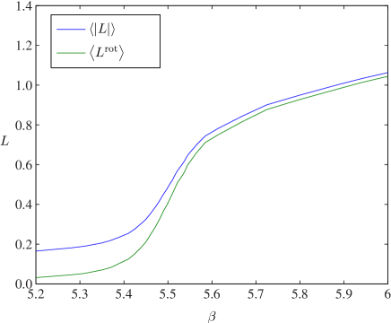
Figure 3: Dependence of the mean modulus of $L$ and the center-transformed and rotated $L$ (see text) on the Wilson coupling $\beta$ on a $4^{3}\times 3$ lattice. The critical coupling is $\beta_{\rm crit}=5.49$

For each $\beta$ between $4\,000$ and $20\,000$ independent configuration have been generated and analyzed. For our relatively small lattices the two order parameters change gradually from the symmetric confined to the broken deconfined phase. Table 1 contains the order parameters for $11$ Wilson couplings.

$\beta$	5.200	5.330	5.440	5.475			5.505	5.530	5.560	5.615	5.725	5.885	6.000
$\langle|L|\rangle$	0.1654	0.1975	0.3050	0.3980			0.5049	0.5939	0.6865	0.7832	0.9007	1.0013	1.0631
$\langle L^{\rm rot}\rangle$	0.0318	0.0615	0.1859	0.3013			0.4296	0.5363	0.6452	0.7513	0.8770	0.9797	1.0444

Table 1: Dependence of the order parameters $|L|$ and $L^{\rm rot}$ on the Wilson coupling $\beta$.

For every independent configuration we calculated the dim$({\mathcal{D}})=2304$ eigenvalues of the Wilson-Dirac operator. Then we averaged the absolute values of the partial traces $\Sigma_{n}$ for every $\beta$ in table 1. In Fig. 4 the ratios

$$R_{n}=\frac{\langle|\Sigma_{n}|\rangle}{\langle|L|\rangle}$$ (28)

are plotted for these $\beta$ as function of the percentage of eigenvalues considered in the partial traces.

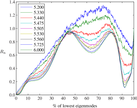
Figure 4: Modulus of the eigenvalue sums starting from the lowest eigenmodes on a $4^{3}\!\times\!3$-lattice near the phase transition. The distinct graphs are labelled with the Wilson coupling $\beta$.

To retain information on the phase of the partial traces and Polyakov loop we used the invariant order parameter constructed in Wozar et al. (2006). Recall that the domain for the traced Polyakov loop is the triangle shown in Fig. 5. The three elements in the center of $SU(3)$ correspond to the corners of the triangle.

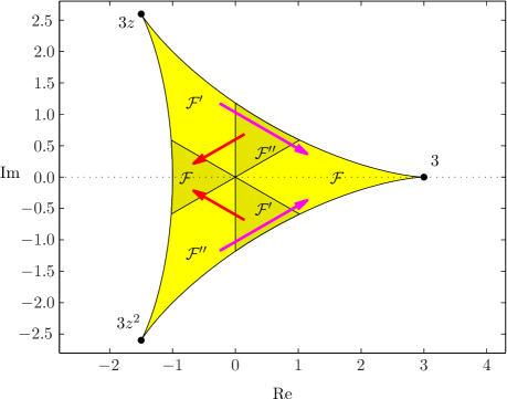
Figure 5: Fundamental domain ${\mathcal{F}}$ of $L$ obtained by identifying $\mbox{\af Z}(3)$ copies according to the depicted arrows.

We divide the domain into the six distinct parts in Fig. 5. The light-shaded region represents the preferred location of the traced Polyakov loop $L$ in the deconfined (ferromagnetic) phase, whereas the dark-shaded region corresponds to the hypothetical anti-center ferromagnetic phase Wipf et al. (2007). In the deconfined phase $L$ points in the direction of a center element whereas it points in the opposite direction in the anti-center phase. To eliminate the superfluous center-symmetry we identify the regions as indicated by the arrows in Fig. 5. This way we end up with a fundamental domain ${\mathcal{F}}$ for the center-symmetry along the real axis. Every $L$ is mapped into ${\mathcal{F}}$ by a center transformation. To finally obtain a real observable we rotate the transformed $L$ inside ${\mathcal{F}}$ onto the real axis. The result is the variable $L^{\rm rot}$ whose sign clearly distinguishes between the different phases. $L^{\rm rot}$ is negative in the anti-center phase, positive in the deconfined phase and zero in the confined symmetric phase. The object $L^{\rm rot}$ is a useful order parameter for the confinement-deconfinement phase transition in gluodynamics Wozar et al. (2006).

We performed the same construction with the partial sums $\Sigma_{n}$ and calculated the ratios for the corresponding Monte-Carlo averages

$$R^{\rm rot}_{n}=\frac{\langle\Sigma^{\rm rot}_{n}\rangle}{\langle L^{\rm rot}\rangle}$$ (29)

for every $\beta$ in table 1 as a function of the percentage of eigenvalues considered in $\Sigma_{n}$.

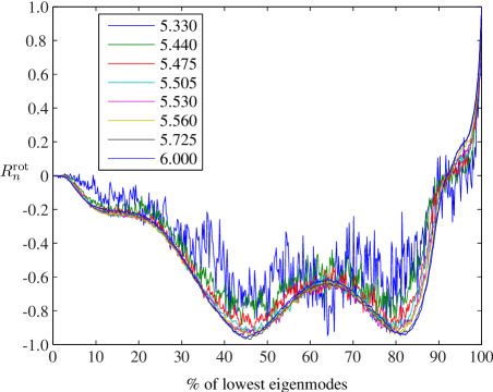
Figure 6: Eigenvalue sums rotated to the fundamental domain starting from the lowest eigenmodes on a $4^{3}\!\times\!3$-lattice near the phase transition. The distinct graphs are labelled with the Wilson coupling.

In Fig. 4 and 6 we observe a universal behavior in the deconfined phase with modulus of the traced Polyakov loop larger than approximately $0.4$. If we include less than $90\%$ of the eigenvalues, then the partial sums $\Sigma_{n}$ have a phase shift of $\pi$ in comparison with $\Sigma=\Sigma_{\rm dim{\mathcal{D}}}$. The last dip in Fig 4 is due to this phase shift and indicates the transition through zero that occurs when $\Sigma_{n}$ changes sign. The same shift and dip has been reported for staggered fermions on a $6^{3}\times 4$ lattice in Bruckmann et al. (2006). For staggered fermions $\Sigma_{n}$ and $\Sigma$ are in phase for $n\geq 0.65\cdot\hbox{dim}({\mathcal{D}})$. For Wilson-Dirac fermions this happens only for $n\geq 0.9\cdot\hbox{dim}({\mathcal{D}})$.

Finite spatial size scaling of partial sums:

We fixed the coupling at $\beta=5.5$ and simulated in the deconfined phase on $N_{\mathrm{s}}^{3}\times 2$-lattices with varying spatial sizes $N_{\mathrm{s}}\in\{3,4,5\}$. For this coupling the systems are deep in the broken phase and we can study finite size effects on the spectral sums.

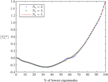
Figure 7: Rotated eigenvalue sums starting from the lowest $\lambda_{p}$ on a $N_{\mathrm{s}}^{3}\!\times\!2$-lattice in the broken phase.

The results for $\Sigma_{n}^{\rm rot}$ are depicted in Fig. 7. We observe that to a high precision $\Sigma_{n}^{\rm rot}$ is approximately independent of the spatial volume. The curves for $N_{\mathrm{s}}=4$ and $5$ are not distinguishable in the plot and as expected $\sum_{k}\bar{z}_{k}{\rm tr}({{}^{z_{k}}\mathcal{D}}^{N_{\mathrm{t}}})$ scales with the spatial volume of the system. An increase of $N_{\mathrm{s}}$ affects the spectra for the untwisted and twisted configurations alike – they only become denser with increasing spatial volume. On the other hand, comparing Fig. 6 and Fig. 7, it is evident that the graph of $\Sigma_{n}^{\rm rot}$ depends very much on the temporal extent of the lattice.

Partial traces $\Sigma_{n}^{(\ell)}$:

The truncated eigenvalue sums (27) with different powers $\ell$ of the eigenvalues show an universal behavior that is nearly independent of the lattice size. The main reason for this universality and in particular the sign of $\Sigma_{n}^{(\ell)}$ is found in the response of the low-lying eigenvalues to twisting the gauge field. It has been observed that for non-periodic boundary conditions (which are gauge-equivalent to twisting the gauge field) the low lying eigenvalues are on the average further away from the origin as compared to periodic boundary conditions (or untwisted gauge fields) Chandrasekharan and Christ (1996); Chandrasekharan and Huang (1996); Stephanov (1996); Gattringer et al. (2002). This statement is very clear for massless staggered fermions with eigenvalues on the imaginary axis. For example, the partial traces

$$\Sigma_{n}^{(1)}\propto\sum_{p=1}^{n}\lambda_{p}+\bar{z}\sum_{p=1}^{n}{{}^{z\!}\lambda}_{p}+z\sum_{p=1}^{n}{{}^{\bar{z}}\lambda}_{p},\qquad|\lambda_{p}|\leq|\lambda_{p+1}|.$$ (30)

with $n\ll\hbox{dim}\,{\mathcal{D}}$ and the traced Polyakov loop have opposite phases. This is explained as follows: all sums in (30) are positive and on the average the last two sums are equal. With $z+\bar{z}=-1$ the last two terms add up to $-\sum{{}^{z\!}\lambda}_{p}$. Since the low lying eigenvalues for the twisted field are further away from the origin as for the untwisted field, the spectral sums (30) are negative for small $n$.

IV Traces of propagators

To suppress the contributions of large eigenvalues we introduce spectral sums $\Sigma^{(\ell)}$ with negative exponents $\ell$. Similar to the Polyakov loop these sums serve as order parameters for the center symmetry. In particular the spectral sums

$$\Sigma^{(-1)}=\frac{1}{\kappa}\sum_{k}{\rm tr}\left(\frac{\bar{z}_{k}}{{{}^{z_{k}}\mathcal{D}}}\right)\quad\hbox{{and}}\quad\Sigma^{(-2)}=\frac{1}{\kappa}\sum_{k}{\rm tr}\left(\frac{\bar{z}_{k}}{{{}^{z_{k}}\mathcal{D}}^{2}}\right)\$$ (31)

are of interest, since they relate to the Green functions of ${\mathcal{D}}$ and ${\mathcal{D}}^{2}$, objects which enter the discussion of the celebrated Banks-Casher relation. Contrary to the ultraviolet-dominated sums with positive $\ell$ are the sums with negative $\ell$ dominated by the eigenvalues in the infrared. The operators $\{{{}^{z}\mathcal{D}},\,z\!\in\!{\mathcal{Z}}\}$ have similar spectra and we may expect that $\kappa\Sigma^{(-1)}$ has a well-behaved continuum limit. Here we consider the partial traces

$$\Sigma^{(-1)}_{n}=\frac{1}{\kappa}\sum_{k}\bar{z}_{k}\sum_{p=1}^{n}\frac{1}{{{}^{z_{k}\!}\lambda}_{p}},\quad\hbox{{and}}\quad\Sigma^{(-2)}_{n}=\frac{1}{\kappa}\sum_{k}\bar{z}_{k}\sum_{p=1}^{n}\frac{1}{({{}^{z_{k}\!}\lambda}_{p})^{2}},\quad|\lambda_{p}|\leq|\lambda_{p+1}|.$$ (32)

Since the Wilson-Dirac operator with flat connection possesses zero-modes we added a small mass $m=0.1$ to the denominators in (32).

Figure 8: The partial spectral sums $\Sigma^{(-1)}_{n}$ for the inverse power and flat connections.

In Fig. 8 the partial sums $\Sigma^{(-1)}_{n}$ on a $4^{3}\times 3$ lattice are plotted. It is seen that for flat connections the $\Sigma^{(-1)}_{n}$ for small $n$ are excellent indicators for the traced Polyakov loop. Thus it is tempting to propose $\Sigma^{(-1)}_{n},\,\Sigma^{(-2)}_{n}$ with $n\ll{\rm dim}{\mathcal{D}}$ as order parameters for the center symmetry. To test this proposal we calculated the partial sums (32), transformed to the fundamental domain and rotated to the real axis, for Monte-Carlo generated configurations on a $4^{3}\times 3$ lattice for various values of $\beta$. The results in Fig. 9 are qualitatively similar to those for the flat connections. Taking into account $10\%$ of the eigenvalues in the IR already yields the asymptotic values $\Sigma^{(-1),{\rm rot}}$ and $\Sigma^{(-2),{\rm rot}}$.

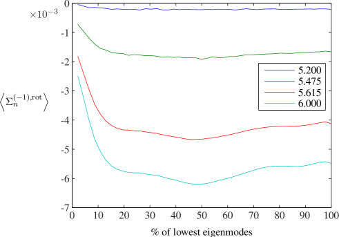
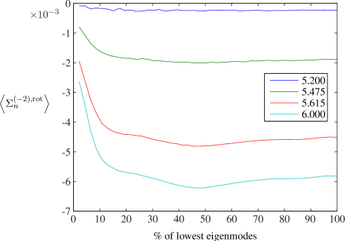
Figure 9: The expectation values of the partial spectral sums $\Sigma^{(-1)}_{n}$ and $\Sigma^{(-2)}_{n}$ rotated to the fundamental domain starting from the lowest eigenvalue on a $4^{3}\times 3$ lattice. The graphs are labelled with $\beta$.

To find an approximate relation between $\Sigma^{(-1)}$ and the traced Polyakov loop we applied the hopping-parameter expansion. To that end one expands the inverse of the Wilson-Dirac operator ${\mathcal{D}}=(m+d)\mathbbm{1}-V$ in powers of $V$,

$${\mathcal{D}}^{-1}=\frac{1}{m+d}\sum_{k}\frac{1}{(m+d)^{k}}\big{[}(m+d)\mathbbm{1}-{\mathcal{D}}\big{]}^{k}.$$ (33)

Inserting this Neumann series into $\Sigma^{(-1)}$ in (31) and keeping the leading term only yields

$$\Sigma^{(-1)}=\frac{(-1)^{N_{\mathrm{t}}}}{(m+d)^{N_{\mathrm{t}}+1}}\,\Sigma^{(1)}+\dots\stackrel{{\scriptstyle(\ref{gattr3})}}{{\approx}}\frac{(-1)^{N_{\mathrm{t}}}}{(m+d)^{N_{\mathrm{t}}+1}}L.$$ (34)

To check whether the expectation values of $\Sigma^{(-1),\rm rot}$ and $L^{\rm rot}$ are indeed proportional to each other we have calculated these values for Monte-Carlo ensembles corresponding to the $11$ Wilson couplings in table 1. The results in Fig. 10 clearly demonstrate that there is such a linear relation.

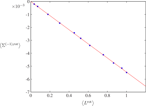
Figure 10: The expectation values of $\Sigma^{(-1),\rm rot}$ as functions of $\langle L^{\rm rot}\rangle$ on a $4^{3}\times 3$ lattice.

A linear fit yields

$$\langle\Sigma^{(-1),\rm rot}\rangle=-0.00545\cdot\langle L^{\mathrm{rot}}\rangle-4.379\cdot 10^{-6}\quad({\rm rmse}=2.978\cdot 10^{-5}).$$ (35)

For massless fermions on a $4^{3}\times 3$ lattice the crude approximation (28) leads to a slope $-0.003906$. This is not far off the slope $-0.00545$ extracted from the Monte-Carlo data.

We have repeated our calculations for the spectral sum $\Sigma^{(-2),\rm rot}$. The corresponding results for the expectation values in Fig. 11 show again a linear relation between the expectation values of this spectral sum and the traced Polyakov loop.

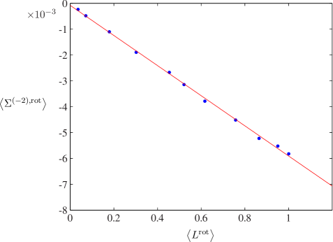
Figure 11: The expectation values of $\Sigma^{(-2),\rm rot}$ as functions of $\langle L^{\rm rot}\rangle$ on a $4^{3}\times 3$ lattice.

This time a linear fit yields $\langle\Sigma^{(-2),\rm rot}\rangle=-0.00582\cdot\langle L^{\mathrm{rot}}\rangle-8.035\cdot 10^{-5}.$

V Exponential spectral sums

After the convincing results for sums of inverse powers of the eigenvalues we analyze the partial exponential spectral sums

$${\mathcal{E}}_{n}=\frac{1}{\kappa}\sum_{k}\bar{z}_{k}\sum_{p=1}^{n}e^{-{{}^{z_{k}\!}\lambda}_{p}} \Longrightarrow {\mathcal{E}}\equiv{\mathcal{E}}_{\rm dim{\mathcal{D}}}=\frac{1}{\kappa}\sum_{k}\bar{z}_{k}\,{\rm tr}\exp\left(-{{}^{z_{k}}\mathcal{D}}\right)$$ (36)

$${\mathcal{G}}_{n}=\frac{1}{\kappa}\sum_{k}\bar{z}_{k}\sum_{p=1}^{n}e^{-|{{}^{z_{k}\!}\lambda}_{p}|^{2}} \Longrightarrow {\mathcal{G}}={\mathcal{G}}_{\rm dim{\mathcal{D}}}=\frac{1}{\kappa}\sum_{k}\bar{z}_{k}\,{\rm tr}\exp\left(-{{}^{z_{k}}\mathcal{D}}^{\dagger}\,{{}^{z_{k}}\mathcal{D}}\right)$$ (37)

In particular the last expression is used in a heat kernel regularization of the fermionic determinant. $\kappa{\mathcal{G}}$ has a well-behaved continuum limit if we enclose the system in a box with finite volume. We computed the partial sums ${\mathcal{G}}_{n}$ for the flat connections and various values

Figure 12: The partial Gaussian sums ${\mathcal{G}}_{n}$ for flat connections with different $L$.

of the traced Polyakov loop. In Fig. 12 we plotted those sums for which $10\%$ or less of the low lying eigenvalues have been included. Similarly as for the sums of negative powers of the eigenvalues we conjecture that the Gaussian sums ${\mathcal{G}}_{n}$ are good candidates for an order parameter in the infrared.

The expectation values of the partial sums ${\mathcal{E}}_{n}^{\rm rot}$ and ${\mathcal{G}}_{n}^{\rm rot}$ for Monte-Carlo generated configurations at four Wilson couplings are plotted in Fig. 13 and Fig. 14.

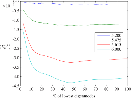
Figure 13: Mean exponential sums ${\mathcal{E}}_{n}^{\rm rot}$ on a $4^{3}\!\times\!3$-lattice near $\beta_{\rm crit}$. The graphs are labelled with $\beta$.

As expected from our studies of flat connections, the Gaussian sums are perfect order parameters for the center symmetry. They are superior to the other spectral sums considered in this paper, since their support is even further at the infrared end of the spectrum. Fig. 15 shows the expectation values $\langle{\mathcal{G}}^{\rm rot}_{n}\rangle$ with only $4.5\%$ or less of the infrared-modes included.

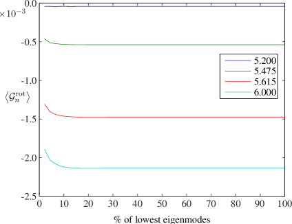
Figure 14: Mean Gaussian sums ${\mathcal{G}}^{\rm rot}_{n}$ on a $4^{3}\!\times\!3$-lattice near $\beta_{\rm crit}$. The graphs are labelled with $\beta$.

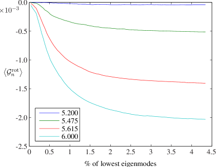
Figure 15: Zooming into Gaussian sums ${\mathcal{G}}_{n}^{\rm rot}$ on a $4^{3}\!\times\!3$-lattice near the phase transition.

The result is again in qualitative agreement with that for flat connections in Fig. 12, although in the Monte-Carlo data the dips are washed out.

The Monte-Carlo results for the expectation values $\langle{\mathcal{E}}^{\rm rot}\rangle$ and $\langle L^{\rm rot}\rangle$ with Wilson couplings in table 1 are depicted in Fig. 16. The quality of the linear fit

$$\langle{\mathcal{E}}^{\rm rot}\rangle=-0.00408\cdot\langle L^{\mathrm{rot}}\rangle+2.346\cdot 10^{-5}\quad({\rm rmse}=1.82\cdot 10^{-5}),$$ (38)

is as good as for the spectral sum $\Sigma^{(-1)}$.

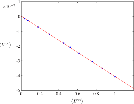
Figure 16: The expectation value of ${\mathcal{E}}^{\rm rot}$ as function of $\langle L^{\rm rot}\rangle$ on a $4^{3}\times 3$ lattice.

To estimate the slope and in particular its dependence on the lattice size we expand the exponentials in ${\mathcal{E}}_{n}$ which results in

$${\mathcal{E}}_{n}=(-)^{N_{\mathrm{t}}}\sum_{p=0}^{\infty}\frac{(-1)^{p}}{(N_{\mathrm{t}}+p)!}\,\Sigma^{(N_{\mathrm{t}}+p)}_{n}.$$ (39)

Since $\Sigma^{(\ell)}$ is proportional to the traced Polyakov loop for $\ell\leq 3N_{\mathrm{t}}$ we conclude that ${\mathcal{E}}={\mathcal{E}}_{{\rm dim}{\mathcal{D}}}$ should be proportional to $L$. We can estimate the proportionality factor as follows: in the Wilson loop expansion of ${\rm tr}\,{\mathcal{D}}^{(N_{\mathrm{t}}+p)}$ only loops winding around the periodic time direction contribute. If we neglect fat loops and only count the straight loops winding once around the periodic time direction, then there are

$$(m+d)^{p}\cdot{N_{\mathrm{t}}+p\choose p}$$ (40)

such loops contributing. Actually, for $p\geq N_{\mathrm{t}}$ there are loops winding several times around the time direction. But these have relatively small entropy and do not contribute much. Hence, with (39) we arrive at the estimate

$${\mathcal{E}}\approx(-1)^{N_{\mathrm{t}}}\sum_{p=0}\frac{(-1)^{p}}{(N_{\mathrm{t}}+p)!}(m+d)^{p}\cdot{N_{\mathrm{t}}+p\choose p}\cdot L=\frac{(-1)^{N_{\mathrm{t}}}}{N_{\mathrm{t}}!}e^{-(m+d)}L.$$ (41)

In $4$ dimensions and for $m=0$ we obtain the approximate linear relation

$$N_{\mathrm{t}}!\,{\mathcal{E}}\approx(-1)^{N_{\mathrm{t}}}\cdot 0.0183\cdot L.$$ (42)

For the linear fit (38) to the MC-data the slope is $3!\cdot 0.00408=0.0245$ instead of $0.0183$.

The Monte-Carlo results for the order parameters $\langle{\mathcal{G}}^{\rm rot}\rangle$ and $\langle L^{\rm rot}\rangle$ with Wilson couplings from table 1 are shown in Fig. 17.

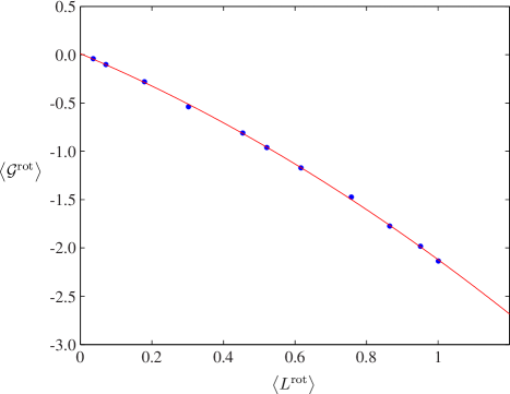
Figure 17: The expectation value of ${\mathcal{G}}^{\rm rot}$ as function of $\langle L^{\rm rot}\rangle$ on a $4^{3}\times 3$ lattice.

In this case the functional dependence is more accurately described by a quadratic function,

$$\langle{\mathcal{G}}^{\rm rot}\rangle=-0.000571\cdot\langle L^{\mathrm{rot}}\rangle^{2}-0.00156\cdot\langle L^{\mathrm{rot}}\rangle+1.061\cdot 10^{-5}\quad({\rm rmse}=1.453\cdot 10^{-5}),$$ (43)

and this relation is very precise. Since in addition $\langle{\mathcal{G}}_{n}^{\rm rot}\rangle\approx\langle{\mathcal{G}}^{\rm rot}\rangle$ already for small $n$ we can reconstruct the order parameter $\langle L^{\rm rot}\rangle$ from the low lying eigenvalues of the Wilson-Dirac operator.

Scaling with $N_{\mathrm{t}}$:

On page III we discussed the finite (spatial) size scaling of the MC expectation values $\langle\Sigma_{n}^{\rm rot}\rangle$. We showed that they converge rapidly to their infinite-$N_{\mathrm{s}}$ limit, see Fig. 7. Here we study how the Gaussian sums ${\mathcal{G}}_{n}$ depend on the temporal extend of the lattice. To that end we performed simulations on larger lattices with fixed $N_{\mathrm{s}}=6$, variable $N_{\mathrm{t}}=2,3,4,5$ and Wilson coupling $\beta=6.5$. We calculated the ratios

$$\tilde{R}^{\rm rot}_{n}=\frac{\kappa}{\langle L^{\rm rot}\rangle}\,\langle{\mathcal{G}}_{n}^{\rm rot}\rangle,$$ (44)

where we multiplied with the extensive factor $\kappa$ in (7) since in the partial sums

$$\tilde{\mathcal{G}}_{n}=\kappa{\mathcal{G}}_{n}=\sum_{k}\bar{z}_{k}\sum_{p=1}^{n}e^{-|{{}^{z_{k}\!}\lambda}_{p}|^{2}}\,,\qquad|\lambda_{p}|\leq|\lambda_{p+1}|.$$ (45)

only a tiny fraction of the $5184$ to $12\,960$ eigenvalues have been included. The order parameter $\langle L^{\rm rot}\rangle$ for the lattices with $N_{\mathrm{t}}=2,\,3,\,4,\,5$ is $1.9474,\,1.40194,\,0.932245,\,0.523142$. In Fig. 18 we plotted the ratios $\tilde{R}^{\rm rot}_{n}$ for $n$ from $1$ up to $100$.

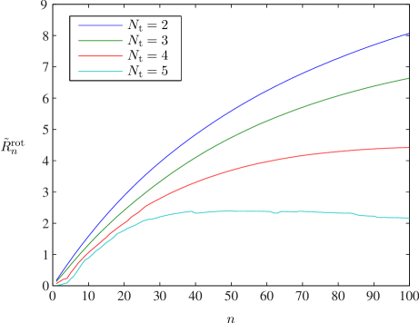
Figure 18: The rations $\tilde{R}^{\rm rot}_{n}$ as function of the number $n$ of IR-eigenvalues included. $100$ eigenvalues corresponds to approximately $1\%$ of all eigenvalues.

Note that on the $6^{3}\times 5$-lattice $n=100$ means less than $0.8\%$ of all $12\,960$ eigenvalues. This figure very much supports our earlier statements about the quality of the order parameters $\langle{\mathcal{G}}_{n}^{\rm rot}\rangle$ or $\langle\tilde{\mathcal{G}}_{n}^{\rm rot}\rangle$.

VI Conclusions

In this paper we studied spectral sums of the type

$${\mathcal{S}}_{n}(f)=\frac{1}{\kappa}\sum_{k}\bar{z}_{k}\sum_{p=1}^{n}f\left({{}^{z_{k}\!}\lambda}_{p}\right)\quad\hbox{{and}}\quad\hat{\mathcal{S}}_{n}(f)=\frac{1}{\kappa}\sum_{k}\bar{z}_{k}\sum_{p=1}^{n}f\left(|{{}^{z_{k}\!}\lambda}_{p}|^{2}\right).$$ (46)

where $\{{{}^{z_{k}\!}\lambda}_{p}\}$ is the set eigenvalues of the Wilson-Dirac operator with twisted gauge field. Summing over all dim$({\mathcal{D}})$ eigenvalues the sums over $p$ become traces such that

$${\mathcal{S}}(f)=\frac{1}{\kappa}\sum_{k}\bar{z}_{k}\,{\rm tr}f\left({{}^{z_{k}}\mathcal{D}}\right)\quad\hbox{{and}}\quad\hat{\mathcal{S}}(f)=\frac{1}{\kappa}\sum_{k}\bar{z}_{k}\,{\rm tr}f\left({{}^{z_{k}}\mathcal{D}}^{\dagger}\,{{}^{z_{k}}\mathcal{D}}\right).$$ (47)

For $f(\lambda)=\lambda^{N_{\mathrm{t}}}$ one finds the spectral sum $\Sigma$ which reproduces the traced Polyakov loop Gattringer (2006). Unfortunately this lattice-result is probably of no use in the continuum limit. Thus we have used functions $f(\lambda)$ which vanish for large (absolute) values of $\lambda$. The corresponding sums are order parameters which get their main contribution from the infrared end of the spectrum. Of all spectral sums considered here, the Gaussian sums ${\mathcal{G}}_{n}$ in (37) define the most efficient order parameters. Besides the ${\mathcal{G}}_{n}$ the spectral sums of inverse powers of eigenvalues are quite useful as well. This observation may be of interest since these sums relate to the Banks-Casher relation.

It remains to investigate the continuum limits of the spectral sums considered in this paper. The properly normalized ${\mathcal{G}}_{n}$ should have a well-behaved continuum limit. With regard to the conjectured relation between confinement and chiral symmetry breaking it would be more interesting to see whether the suitably normalized sums $\Sigma^{(-1)}$ or/and $\Sigma^{(-2)}$ can be defined in the continuum theory. Clearly, the answer to this interesting question depends on the dimension of spacetime.

Acknowledgments: We thank Georg Bergner, Falk Bruckmann, Christof Gattringer, Tobias Kästner and Sebastian Uhlmann for interesting discussions. This project has been supported by the DFG, grant Wi 777/8-2.

References

- Polyakov (1978) A. M. Polyakov, Phys. Lett. B72, 477 (1978).
- Susskind (1979) L. Susskind, Phys. Rev. D20, 2610 (1979).
- Yaffe and Svetitsky (1982) L. G. Yaffe and B. Svetitsky, Phys. Rev. D26, 963 (1982).
- Wozar et al. (2006) C. Wozar, T. Kaestner, A. Wipf, T. Heinzl, and B. Pozsgay, Phys. Rev. D74, 114501 (2006), eprint hep-lat/0605012.
- Leutwyler and Smilga (1992) H. Leutwyler and A. Smilga, Phys. Rev. D46, 5607 (1992).
- Banks and Casher (1980) T. Banks and A. Casher, Nucl. Phys. B169, 103 (1980).
- Schafer and Shuryak (1998) T. Schafer and E. V. Shuryak, Rev. Mod. Phys. 70, 323 (1998), eprint hep-ph/9610451.
- Kogut et al. (1983) J. B. Kogut et al., Phys. Rev. Lett. 50, 393 (1983).
- Karsch (2002) F. Karsch, Lect. Notes Phys. 583, 209 (2002), eprint hep-lat/0106019.
- Gattringer (2006) C. Gattringer, Phys. Rev. Lett. 97, 032003 (2006), eprint hep-lat/0605018.
- Bruckmann et al. (2006) F. Bruckmann, C. Gattringer, and C. Hagen (2006), eprint hep-lat/0612020.
- Wipf et al. (2007) A. Wipf, T. Kaestner, C. Wozar, and T. Heinzl, SIGMA 3, 006 (2007), eprint hep-lat/0610043.
- Chandrasekharan and Christ (1996) S. Chandrasekharan and N. H. Christ, Nucl. Phys. Proc. Suppl. 47, 527 (1996), eprint hep-lat/9509095.
- Chandrasekharan and Huang (1996) S. Chandrasekharan and S.-z. Huang, Phys. Rev. D53, 5100 (1996), eprint hep-ph/9512323.
- Stephanov (1996) M. A. Stephanov, Phys. Lett. B375, 249 (1996), eprint hep-lat/9601001.
- Gattringer et al. (2002) C. Gattringer, P. E. L. Rakow, A. Schafer, and W. Soldner, Phys. Rev. D66, 054502 (2002), eprint hep-lat/0202009.