Mixed Action Lattice Spacing Effects on the Nucleon Axial Charge

Abstract

We study the nucleon axial charge in the chiral perturbation theory for a mixed lattice action of Ginsparg-Wilson valence quarks and staggered sea quarks. In particular, we investigate the lattice spacing $a^{2}$-dependence of the neutron to proton axial transition matrix element. By using the known low-energy constants (LEC’s) and an estimated value of a new LEC which appears in the calculation, we see a large lattice spacing effect on $g_{A}$.

I Introduction

Lattice QCD, the only known first principle non-perturbative approach to QCD, has made a dramatic progress in the last decade because of the increasing power in the computing resources and the improvement of the numerical algorithms for the simulations. Today fully dynamical lattice QCD simulations together with effective theories enable one to make first principle predictions of hadronic physics. Recently, a so-called mixed-action lattice simulation using different kind of fermions in the valence and sea sectors has gained attention because these simulations can reach the pion masses as low as $300{\text{MeV}}$ Aubin et al. (2004c, 2005a); Silas:2005 ; Edward:2005 ; Silas:2006.1 ; Silas:2006.2 ; Silas:2006.3 ; Silas:2006.4 ; Edward:2005.1 ; Negele:2006.1 ; Negele:2006.2 . In particular, despite the controversy of the validity of the fourth root trick used to overcome the fermion taste doubling problem of the staggered fermions, the lattice calculations using Ginsparg-Wilson valence quarks in staggered sea quarks has become popular because many quantitative results are obtained Aubin et al. (2004c, 2005a); Silas:2005 ; Edward:2005 ; Silas:2006.1 ; Silas:2006.2 ; Silas:2006.3 ; Silas:2006.4 . Further, the publicly available MILC configurations Bernard et al. (2001) have encouraged the use of lattice calculations with dynamical staggered fermions.

The lattice action can be described by Symanzik action Symanzik:1983dc ; Symanzik:1983gh which is based on the symmetries of the underlying lattice theory and can be organized in powers of the lattice spacing $a$:

$${\mathcal{L}}_{\text{Sym}}={\mathcal{L}}+a\,{\mathcal{L}}^{(5)}+a^{2}\,{\mathcal{L}}^{(6)}+\dots\,,$$ (1)

where ${\mathcal{L}}^{(n)}$ represents the contribution from dimension-$n$ operators. The symmetries of the lattice action are respected by the Symanzik Lagrangian ${\mathcal{L}}_{\text{Sym}}$ order-by-order in $a$. In order to address lattice spacing corrections, based on the Symanzik action, several mixed-action chiral perturbation theories are developed to investigate the systematic errors which arise from lattice simulations due to the non-vanishing lattice spacing Bar et al. (2003, 2004); Silas:2003 ; bct0501 ; OBar:2005 ; bct0508 . These mixed-action chiral perturbation theories provide a way to test the results from the lattice calculations using the mixed lattice action and vice-versa.

The nucleon axial charge, $g_{A}$, is an important quantity in QCD which quantifies the spontaneous chiral symmetry breaking. Since its value is known to a very high precision in experiments PDG:2006 , it can be used as a very good test for the first principle lattice calculations. This quantity of hadronic physics has been studied extensively in both lattice simulations and chiral perturbation theory Edward:2005 ; Jenkins:1991jv ; Jenkins:1991es ; Blum:2004 ; Khan:2005 ; Borasoy:1999 ; Zhu:2001 ; s&m:2002 ; s&m:2004 . Although to perform the lattice simulations to calculate $g_{A}$ is straightforward, some controversy remains. For example, the $g_{A}$ obtained from lattice simulations has raised the controversy of the possibility of large volume effects in the chiral limit Jaffe:2002 ; Cohen:2002 . Recently, using the mixed-action of Domain Wall valence quarks with staggered sea quarks, Edward:2005 obtained a nice result of $g_{A}$ which seems to match nicely with the prediction from chiral perturbation theory and it is expected that the future data might be able to make contact with experiment via extrapolation. On the other hand, in Edward:2005 , the discretization errors in computing $g_{A}$ using the mixed-action might be overlooked. With the advent of mixed-action $\chi$PT OBar:2005 and extension to the baryon sector bct0508 , it is surprising that lattice spacing effects on the nucleon axial charge have not been addressed. In this paper we address this issue mentioned above, namely, we use the mixed-action chiral perturbation theory to study the lattice-spacing dependence of $g_{A}$. In particular, we found that it depends on the unphysical low energy constant $g_{1}$ and a new unknown LEC for which the actual value must be obtained from lattice calculations.

This paper is organized as follow. In Section $2$, we briefly review the chiral perturbation theory of Ginsparg-Wilson valence quarks in staggered sea. In particular, we will put emphasis on the lattice-spacing $a$ dependence of the mixed-action Lagrangian. Next, in Section $3$, we will construct the axial-vector current from the mixed-action Lagrangian and compute the $pn$ matrix element of the axial-vector current. Further we will compare the results obtained in the presence and absence of lattice-spacing $a$. Finally we conclude in Section $4$. For completeness, we include some standard functions which arise in this calculation in the Appendix.

II Chiral Lagrangian

To address the finite lattice spacing issue, with the pioneering work in Sharpe and Singleton (1998); Lee and Sharpe (1999), Rupak and Shoresh (2002); Bar et al. (2003, 2004) have extended the $\chi$PT in the meson sector. This finite lattice spacing artifacts has also be investigated in staggered $\chi$PT for the mesons Aubin and Bernard (2003a, b); Sharpe:2004is and the mixed-action PQ$\chi$PT Silas:2003 ; OBar:2005 ; bct0501 ; bct0508 . To address the finite lattice spacing effects, one utilizes a dual expansion in the quark masses and lattice spacing with the usual energy scale Silas:2003 ; Bar et al. (2004):

$$m_{q}\ll\Lambda_{QCD}\ll\frac{1}{a}\,,$$ (2)

and the following power counting scheme bct0508 :

$${\varepsilon}^{2}\sim\begin{cases}m_{q}/{\Lambda}_{QCD}\\ a^{2}{\Lambda}_{QCD}^{2}\end{cases}\,,$$ (3)

which is relevant for current improved staggered quarks simulations.

In this section, we briefly introduce the chiral perturbation theory of the partially-quenched mixed-action theory. In particular, we focus on the mixed-action of Ginsparg-Wilson valence quarks in staggered sea quarks. We only write the chiral Lagrangian of the associated mixed-action theory and do not go into the detail of how this chiral Lagrangian can be constructed from the Symanzik Lagrangian since the detail of the procedure can be found in the references cited above. For our purpose in this paper, we only need to keep in mind that ${\mathcal{L}}^{(5)}=0$ and the taste-symmetry breaking and $SO(4)$ breaking operators will not enter at the order we calculate the axial-vector current matrix element bct0508 .

II.1 Mesons

In the following, the strange quark mass is assumed to be fixed to its physical value, therefore one can use two-flavor theory and does not need to worry about the extrapolation in the strange quark mass. The lattice action we consider here is built from $2$ flavors of Ginsparg-Wilson valence quarks and $2$ flavors of staggered sea quarks. In the continuum limit, the Lagrangian is just the partially quenched Lagrangian which is given by:

$${\mathcal{L}}={\overline{Q}}D\hskip-6.49994pt/\,Q+{\overline{Q}}m_{q}Q\,,$$ (4)

where the quark fields appears as a vector $Q$ with entries given by:

$$Q=(u,d,j_{1},j_{2},j_{3},j_{4},l_{1},l_{2},l_{3},l_{4},\tilde{u},\tilde{d},)^{T}\,.$$ (5)

and transforms in the fundamental representation of the graded group $SU(10|2)$. Notice the fermion doubling has produced four tastes for each flavor $(j,l)$ of staggered sea quark. The partially quenched generalization of the mass matrix $m_{q}$ in the isospin limit is given by:

$$m_{q}=\text{diag}(m_{u},m_{u},m_{j}\xi_{I},m_{j}\xi_{I},m_{u},m_{u})\,,$$ (6)

with $\xi_{I}$ as the $4$ x $4$ taste identity matrix. The low-energy effective theory of the theory we consider above is written in terms of the pseudo-Goldstone mesons emerging from spontaneous symmetry breaking which are realized non-linearly in an $U(10|2)$ matrix exponential $\Sigma$

$$\Sigma=\exp\left(\frac{2i\Phi}{f}\right)=\xi^{2}\,.$$ (7)

To the order (next-to-leading order) we work in investigating the $a^{2}$-dependence of the matrix element of the axial-vector current between nucleons, the relevant partially-quenched chiral perturbation theory Lagrangian for the mesons up to order $O(\epsilon^{2})$ is given by:

$${\mathcal{L}}=\frac{f^{2}}{8}\text{str}\left(\partial_{\mu}\Sigma^{\dagger}\partial_{\mu}\Sigma\right)-{\lambda}\,\text{str}\left(m_{q}\Sigma^{\dagger}+m_{q}^{\dagger}\Sigma\right)+\frac{1}{6}\mu_{0}^{2}\,(\text{str}\,\Phi)^{2}+a^{2}\mathcal{V}\,.$$ (8)

where

$$\Phi=\left(\begin{array}[]{cc}M&\chi^{\dagger}\\ \chi&\tilde{M}\end{array}\right)\,,$$ (9)

$f=132$ MeV, the str() denotes a graded flavor trace and $\Sigma$ is defined in (7). The $M$, $\tilde{M}$, and $\chi$ are matrices of pseudo-Goldstone bosons and pseudo-Goldstone fermions, for example, see s&m:2002 . The potential $\mathcal{V}$ contains the effects of dimension-$6$ operators in the Symanzik action OBar:2005 . Expanding the Lagrangian in Eq. (8) to the leading order, one can determine the meson masses needed for the calculations of baryon observables. In particular, the relevant mesons needed for the axial-vector current matrix element calcualtions are the valence pion, mesons made of $S_{i}\overline{V}$ with one staggered sea quark $S_{i}$ of flavor $S$ and quark taste $i$ and a Ginsparg-Wilson valence quark $\overline{V}$ and finally mesons with two staggered quarks in a flavor-neutral, taste-singlet combination. The associated masses to the lowest order for the latter two mesons can be written in terms of the valence pion mass $m^{2}_{VV}$ which can be determined from the valence spectroscopy and the pseudoscalar taste pion mass $m^{2}_{SS}$ which the mass can be learned from the MILC spectroscopy and are given by:

$$m_{SV}^{2} =\frac{m^{2}_{SS}+m^{2}_{VV}}{2}+\frac{16\,a^{2}\,C_{\text{mix}}}{f^{2}}\,,$$ (10)

$$m_{SS,I}^{2} =m^{2}_{SS}+\frac{64\,a^{2}}{f^{2}}(C_{3}+C_{4})\,,$$

where $C_{\text{mix}}$ and $C_{3}+C_{4}$ are the parameters in the potential $\mathcal{V}$. Since these masses are independent of the quark taste, we do not specify the taste index in (10). Notice the flavor singlet field $\Phi$ is rendered heavy by the $U(1)_{A}$ anomaly and can been integrated out in PQ$\chi$PT. However, the propagator of the flavor-neutral field deviates from a simple pole form Sharpe and Shoresh (2001). Since only the valence-valence flavor-neutral propagators are needed for our later calculations, for $V,V^{\prime}=u,d$, the leading-order $\eta_{V}\eta_{V^{\prime}}$ propagator in the isospin limit is given by s&m:2002 :

$${\cal G}_{\eta_{V}\eta_{V^{\prime}}}=\frac{i\delta_{VV^{\prime}}}{q^{2}-m^{2}_{VV}+i\epsilon}-\frac{i}{2}\frac{\left(q^{2}-m^{2}_{SS,I}\right)}{\left(q^{2}-m^{2}_{VV}+i\epsilon\right)^{2}}\,,$$ (11)

One can further show that these propagators can be conveniently rewritten in a compact form which will be useful in our later calculations:

$${\cal G}_{\eta_{V}\eta_{V^{\prime}}}={\delta}_{VV^{\prime}}P_{V}+{\cal H}_{VV}\left(P_{V},P_{V}\right)\,,$$ (12)

where

$$\qquad P_{V}\ =\ {i\over q^{2}-m_{VV}^{2}+i\epsilon}\,,\ \ \ {\mathcal{H}}_{VV}(A,A)=\frac{1}{2}\Big{[}\,(m_{SS,I}^{2}-m_{VV}^{2})\frac{\partial}{\partial m_{VV}^{2}}A\,-\,A\Big{]}$$ (13)

In writing (13), we have used $A=A(m^{2}_{VV})$.

II.2 Baryon

As has been shown in bct0508 , to $O(\epsilon^{2})$, the free Lagrangian for the $\bf{572}$-dimensional super-multiplet ${\mathcal{B}}^{ijk}$ and the $\bf{340}$-dimensional super-multiplet ${\mathcal{T}}_{\mu}^{ijk}$ fields in the mixed-action $SU(10|2)$ partially quenched $\chi$PT has the same form as in quenched and partially quenched theories Labrenz:1996jy ; MSavage:2002 ; s&m:2002 with the addition of new lattice-spacing dependent terms:

$${\mathcal{L}} = i\left({\overline{{\mathcal{B}}}}v\cdot{\mathcal{D}}{\mathcal{B}}\right)+2{\alpha}^{(PQ)}_{M}\left({\overline{{\mathcal{B}}}}{\mathcal{B}}{\mathcal{M}}_{+}\right)+2{\beta}^{(PQ)}_{M}\left({\overline{{\mathcal{B}}}}{\mathcal{M}}_{+}{\mathcal{B}}\right)+2\sigma^{(PQ)}_{M}\left({\overline{{\mathcal{B}}}}{\mathcal{B}}\right)\text{str}\left({\mathcal{M}}_{+}\right)+a^{2}\mathcal{V}_{{\mathcal{B}}}$$

$$- i\left({\overline{{\mathcal{T}}}}^{\mu}v\cdot{\mathcal{D}}{\mathcal{T}}_{\mu}\right)+{\Delta}\left({\overline{{\mathcal{T}}}}^{\mu}{\mathcal{T}}_{\mu}\right)-2{\gamma}^{(PQ)}_{M}\left({\overline{{\mathcal{T}}}}^{\mu}{\mathcal{M}}_{+}{\mathcal{T}}_{\mu}\right)-2{\overline{\sigma}}^{(PQ)}_{M}\left({\overline{{\mathcal{T}}}}^{\mu}{\mathcal{T}}_{\mu}\right)\text{str}\left({\mathcal{M}}_{+}\right)+a^{2}\mathcal{V}_{{\mathcal{T}}}\,.$$

The baryon potentials $\mathcal{V}_{\mathcal{B}}$ and $\mathcal{V}_{\mathcal{T}}$ in (II.2) arise from the operators in ${\mathcal{L}}^{(6)}$ of the Symanzik Lagrangian. In the baryon Lagrangian, the mass operator is defined by:

$${\mathcal{M}}_{+}=\frac{1}{2}\left(\xi^{\dagger}m_{Q}\xi^{\dagger}+\xi m_{Q}\xi\right).$$ (15)

and the parameter ${\Delta}\sim{\varepsilon}{\Lambda}_{\chi}$ is the mass splitting between the $\bf{572}$ and $\bf{340}$ in the chiral limit. The parenthesis notation used in Eq. (II.2) is that of Labrenz:1996jy . Further, the embeding of the octet and decuplet baryons in their super-multiplets is the same as before MSavage:2002 ; s&m:2002 . The Lagrangian describing the interactions of the ${\mathcal{B}}^{ijk}$ and ${\mathcal{T}}_{\mu}^{ijk}$ with the pseudo-Goldstone mesons in the mixed-action is again the same as in the partially quenched theories s&m:2002 with a new $a^{2}$-dependence term:

$${\cal L} = 2{\alpha}\left({\overline{{\mathcal{B}}}}S^{\mu}{\mathcal{B}}A_{\mu}\right)+2{\beta}\left({\overline{{\mathcal{B}}}}S^{\mu}A_{\mu}{\mathcal{B}}\right)+2{\mathcal{H}}\left({\overline{{\mathcal{T}}}}^{\nu}S^{\mu}A_{\mu}{\mathcal{T}}_{\nu}\right)$$ (16)

$$+ \sqrt{\frac{3}{2}}{\mathcal{C}}\left[\left({\overline{{\mathcal{T}}}}^{\nu}A_{\nu}{\mathcal{B}}\right)+\left({\overline{{\mathcal{B}}}}A_{\nu}{\mathcal{T}}^{\nu}\right)\right]+a^{2}{\mathcal{L}}^{(6)}_{int}\,.$$

The axial-vector and vector meson fields $A_{\mu}$ and $V_{\mu}$ are defined by: $A^{\mu}=\frac{i}{2}\left(\xi\partial^{\mu}\xi^{\dagger}-\xi^{\dagger}\partial^{\mu}\xi\right)$ and $V^{\mu}=\frac{1}{2}\left(\xi\partial^{\mu}\xi^{\dagger}+\xi^{\dagger}\partial^{\mu}\xi\right)$. The latter appears in Eq. (II.2) for the covariant derivatives of ${\mathcal{B}}_{ijk}$ and ${\mathcal{T}}_{ijk}$ that both have the form

$$({\mathcal{D}}^{\mu}{\mathcal{B}})_{ijk}=\partial^{\mu}{\mathcal{B}}_{ijk}+(V^{\mu})^{l}_{i}{\mathcal{B}}_{ljk}+(-)^{\eta_{i}(\eta_{j}+\eta_{m})}(V^{\mu})^{m}_{j}{\mathcal{B}}_{imk}+(-)^{(\eta_{i}+\eta_{j})(\eta_{k}+\eta_{n})}(V^{\mu})^{n}_{k}{\mathcal{B}}_{ijn}.$$ (17)

The vector $S^{\mu}$ is the covariant spin operator Jenkins:1991jv ; Jenkins:1991es and $a^{2}{\mathcal{L}}^{(6)}_{int}$ is from the operators in ${\mathcal{L}}^{(6)}$ of the Symanzik Lagrangian. As we will see later, the explicit form of this term is not required in our calculations. The effective axial-vector current from $a^{2}{\mathcal{L}}^{(6)}_{int}$ can be obtained by a simple argument. The parameters that appear in the mixed-action PQ$\chi$PT Lagrangian can be related to those in $\chi$PT by matching. Further, since QCD is contained in the fourth-root of the sea-sector of the theory, one should restrict oneself to one taste for each flavor of staggered sea quark when performing the matching. To be more specific, one restricts to the $q_{S}q_{S}q_{S}$ sector bct0508 and compares the mixed-action PQ$\chi$PT Lagrangian obtained with the $\chi$PT. With this identification and matching procedure, one finds s&m:2002 :

$$\alpha_{M} = {2\over 3}\alpha_{M}^{(PQ)}-{1\over 3}\beta_{M}^{(PQ)}\,,\quad\ \sigma_{M}\ =\ \sigma_{M}^{(PQ)}+{1\over 6}\alpha_{M}^{(PQ)}+{2\over 3}\beta_{M}^{(PQ)}$$

$$\gamma_{M} = \gamma_{M}^{(PQ)}\,,\quad\ \overline{\sigma}_{M}\ =\ \overline{\sigma}_{M}^{(PQ)}\,.$$ (18)

Further, when restricting to the tree level, from (16) one also finds s&m:2002 :

$$\alpha = {4\over 3}g_{A}\ +\ {1\over 3}g_{1}\,,\ \ \ \beta\ =\ {2\over 3}g_{1}-{1\over 3}g_{A}\,,\ \ \ {\cal H}\ =\ g_{\Delta\Delta}\,,\ \ \ {\cal C}\ =\ -g_{\Delta N}\,,$$ (19)

and $g_{X}=0$.

III The Axial-Vector Current

The matrix element of the axial-vector current, $\overline{q}\tau^{a}\gamma_{\mu}\gamma_{5}q$, have been studied extensively both on the lattice Edward:2005 ; Blum:2004 ; Khan:2005 and $\chi$PT Jenkins:1991jv ; Jenkins:1991es ; Borasoy:1999 ; Zhu:2001 ; s&m:2002 ; s&m:2004 . For our convention, we will follow bct0412 ; bct0504 and use the following charge matrix for the flavor-changing current in extending the isovector axial current $\overline{Q}\overline{\tau}^{a}\gamma_{\mu}\gamma_{5}Q$ to PQQCD since we are interested in the neutron to proton axial transition:

$$\overline{\tau}^{+}=(0,1,0,0,0,....,0)\,.$$ (20)

With this convention, at leading order, the flavor-changing axial current is given as s&m:2002 :

$${}^{(PQ)}j_{\mu,5}^{+} \rightarrow\,2\alpha\ \left(\overline{\cal B}S_{\mu}{\cal B}\ {\overline{\tau}^{+}_{\xi+}}\right)\ +\ 2\beta\ \left(\overline{\cal B}S_{\mu}\ {\overline{\tau}^{+}_{\xi+}}{\cal B}\right)\ +\ 2{\cal H}\left(\overline{\cal T}^{\nu}S_{\mu}\ {\overline{\tau}^{+}_{\xi+}}{\cal T}_{\nu}\right)$$ (21)

$$\ +\ \sqrt{3\over 2}{\cal C}\left[\ \left(\overline{\cal T}_{\mu}\ {\overline{\tau}^{+}_{\xi+}}{\cal B}\right)\ +\ \left(\overline{\cal B}\ {\overline{\tau}^{+}_{\xi+}}{\cal T}_{\mu}\right)\ \right]\ \ +\ a^{2}j^{+}_{a\mu,5}\,\ldots.$$

where $\overline{\tau}^{+}_{\xi+}\ =\ {1\over 2}\left(\xi\overline{\tau}^{+}\xi^{\dagger}+\xi^{\dagger}\overline{\tau}^{+}\xi\right)$ and $j^{+}_{a\mu,5}$ is obtained from ${\mathcal{L}}^{(6)}_{int}$ in (16). Notice since the insertion of the mass matrix will be at $O(\epsilon^{4})$, we only need to take the tree level contribution from $a^{2}J^{+}_{a\mu,5}$ into our calculation. Therefore, although there are a lot of terms in the axial current arise from the $a^{2}$ corrections to the lattice operator itself, the net contributions to the current $j^{+}_{a\mu,5}$ can be effectively written as:

$$j^{+}_{a\mu,5}\,\overset{\text{eff}}{=}\,2C_{a}\ \left(\overline{\cal B}S_{\mu}{\cal B}\ {\overline{\tau}^{+}_{\xi+}}\right)\ +\ 2C^{\prime}_{a}\ \left(\overline{\cal B}S_{\mu}\ {\overline{\tau}^{+}_{\xi+}}{\cal B}\right)\,.$$ (22)

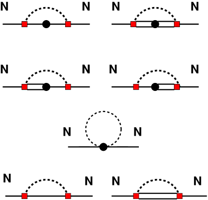
Figure 1: The one-loop diagrams which contribute to the leading non-analytic terms of the nucleon axial transition matrix element. Mesons are represented by a dashed line while the single and double lines are the symbols for a nucleon and a decuplet respectively. The solid circle is an insertion of the axial current operator and the solid squares are the couplings given in (16). The wave function renormalization diagrams are depicted by the two diagrams at the bottom row.

The calculation of the matrix element of the neutron to proton axial transition at next-to-leading order is $O(\epsilon^{3})$ in our power counting. These leading non-analytic terms are from the one-loop diagrams shown in Fig 1. To obtain the complete $O(\epsilon^{3})$ calculation, from our power counting scheme: $\epsilon^{2}\sim a^{2}\Lambda^{2}_{Q}CD$ and $\epsilon^{2}\sim m_{q}/\Lambda_{QCD}$, we see that in addition to taking the $a^{2}$-dependence of the loop meson masses into our calculation, we must evaluate the $j^{+}_{a\mu,5}$ at tree level. After carrying out the calculation, one finds:

$$\langle p|j^{+}_{\mu,5}|n\rangle = \Big{[}\ \Gamma_{pn}\,+\,c_{pn}\ \Big{]}\ 2\overline{U}_{p}S_{\mu}U_{n}\,,$$ (23)

where $c_{pn}$’s are from the contributions of local counterterms involving one insertion of mass matrix $m_{Q}$ and $\Gamma_{pn}$ is given by:

$$\qquad\qquad\Gamma_{pn} = \,g_{A}+a^{2}C^{\prime}-\frac{4}{3f^{2}}\,\Bigg{[}\,\,g_{A}^{3}\frac{3}{2}\Big{(}\,2R_{1}(m_{VS},\mu)\,+\,2A(m_{SS,I})\,\Big{)}\,\,\qquad\qquad$$ (24)

$$- g_{1}^{3}\frac{1}{8}\Big{(}\,R_{1}(m_{VV},\mu)\,-\,R_{1}(m_{VS},\mu)\,\Big{)}\,+\,\frac{3}{2}g_{A}R_{1}(m_{VS},\mu)\,$$

$$- g_{A}^{2}g_{1}\Big{(}\,2R_{1}(m_{VV},\mu)\,-\,2R_{1}(m_{VS},\mu)\,-\,6A(m_{SS,I})\Big{)}\,$$

$$- g_{A}g_{1}^{2}\Big{(}\,\frac{17}{8}R_{1}(m_{VV},\mu)\,-\,\frac{17}{8}R_{1}(m_{VS},\mu)\,-\,3A(m_{SS,I})\Big{)}$$

$$- g_{\Delta N}^{2}g_{1}\frac{4}{9}\Big{(}\,N_{1}(m_{VV},\Delta,\mu)\,-\,N_{1}(m_{VS},\Delta,\mu)\,\Big{)}\,$$

$$+ g_{\Delta N}^{2}g_{\Delta\Delta}\frac{60}{81}\Big{(}\,J_{1}(m_{VV},\Delta,\mu)\,+\,\frac{2}{3}J_{1}(m_{VS},\Delta,\mu)\,\Big{)}$$

$$- g_{\Delta N}^{2}g_{A}\Big{(}\,\frac{16}{9}\Big{\{}N_{1}(m_{VV},\Delta,\mu)+N_{1}(m_{VS},\Delta,\mu)\Big{\}}$$

$$- 2\Big{\{}J_{1}(m_{VV},\Delta,\mu)+J_{1}(m_{VS},\Delta,\mu)\Big{\}}\,\Big{)}\,\Bigg{]}$$

where $C^{\prime}=C_{a}+C^{\prime}_{a}$, the functions $J_{1}(m,\Delta,\mu)$, $R_{1}(m,\mu)$, $N_{1}(m,\Delta,\mu)$ are defined in the Appendix, $\Delta$ is the $\Delta$-nucleon mass splitting, $m_{ab}$ are given in (10) and lastly, the function $A(m_{SS,I})$ is given by:

$$A(m_{SS,I})=\frac{1}{32\pi^{2}}\Big{(}m^{2}_{SS,I}-m^{2}_{VV}\Big{)}\Big{[}\,\log\frac{m^{2}_{VV}}{\mu^{2}}\,+\,1\,\Big{]}$$ (25)

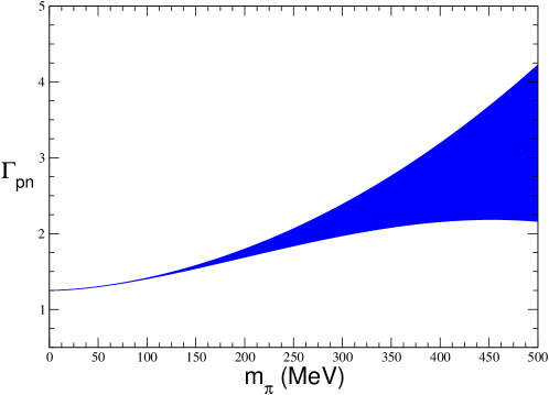
Figure 2: $\Gamma_{pn}\rightarrow g_{A}$ in the chiral limit. Here the physical value of $g_{A}$ is set to be $1.25$. The band structure indicates the variation of $g_{A}$ due to the bounds on $g_{\Delta\Delta}$ and $g_{\Delta N}$.

All of the couplings in eq. (24) take their chiral-limit values. It is easy to see that all the $a^{2}$-dependence in (24) is contained in $m_{VS}$, $m_{SS,I}$ and $a^{2}C^{\prime}$. Notice with our $R_{1}(m,\mu)$, $J_{1}(m,\Delta,\mu)$ and $N_{1}(m,\Delta,\mu)$ we have subtracted off the chiral and continuum limit values of the loop diagrams by hand. This corresponds to a renormalization of the tree level coefficients, and produces $g_{A}$ which is the chiral limit value (Fig 2).

The lattice spacing dependence in Eq. (24) is completely determined by three parameters, namely, $C_{\text{mix}}$ and $C_{3}+C_{4}$, and a new unknown low energy constant $C^{\prime}$. In order to investigate the $a^{2}$-dependence of $np$ axial transition matrix element, in Fig 3, we have taken the unquenched limit in which $m_{VV}=m_{SS}$ and plotted (24) at two different lattice spacing $a=0.12{\text{fm}}$ and $a=0$ with the pion mass varying from $1{\text{MeV}}$ to $500{\text{MeV}}$. In the figure, $g_{A}$ is set to be $1.25$ and the low-energy constants $g_{1}$, $g_{\Delta N}$, $g_{\Delta\Delta}$ are allowed to vary within their reasonably known bounds:: $-1\leq g_{1}\leq 1$, $1.0\leq|g_{\Delta N}|\leq 2.0$ and $2.5\leq|g_{\Delta\Delta}|\leq 3.5$. Further, $C_{\text{mix}}$ is estimated to be $4.5{\text{fm}}^{-6}\leq C_{\text{mix}}\leq 9.5{\text{fm}}^{-6}$ bct:0607 and $C_{3}+C_{4}$ is determined as $C_{3}+C_{4}=2.34{\text{fm}}^{-6}$ Aubin et al. (2004c). Finally, since $C^{\prime}$ is assumed to be of natural size which is $\Lambda^{2}_{QCD}\sim 2.3{\text{fm}}^{-2}$, we have used $-3{\text{fm}}^{-2}\leq C^{\prime}\leq 3{\text{fm}}^{-2}$ for the figure. However, keep in mind that the actual value of $C^{\prime}$ must be determined from lattice calculations.

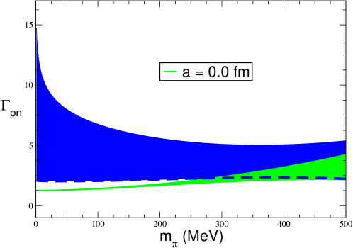
Figure 3: In this figure, we have plotted $\Gamma_{pn}$ as a function of $m_{\pi}$. The green band stands for the band with $a=0$ while the blue band are the $\Gamma_{pn}$ obtained from $g_{A}=1.25$, $C_{3}+C_{4}=2.34{\text{fm}}^{-6}$, reasonably known bounds on $g_{1}$, $g_{\Delta N}$ and $g_{\Delta\Delta}$: $-1\leq g_{1}\leq 1$, $1.0\leq|g_{\Delta N}|\leq 2.0$, $2.5\leq|g_{\Delta\Delta}|\leq 3.5$, a natural estimated value for $C_{\text{mix}}$: $4.5{\text{fm}}^{-6}\leq C_{\text{mix}}\leq 9.5{\text{fm}}^{-6}$, and finally a natural variation of $C^{\prime}$: $-3{\text{fm}}^{-2}\leq C^{\prime}\leq 3{\text{fm}}^{-2}$. The lattice spacing $a$ for the blue band is fixed to be $0.12{\text{fm}}$.

From the figure, we indeed see a large lattice spacing dependence for $\Gamma_{pn}$. One might be concerned that the correction at the chiral limit is sufficiently large that the $\chi$PT prediction might be breaking down. Further, the band at the chiral limit does not cover the value of $1.25$ which is the expected $g_{A}$ at $m_{\pi}\sim 0$. We point out that with $a=0.12{\text{fm}}$, the mass square corrections to the $VS$ and $SS,I$ mesons are around $(400{\text{MeV}})^{2}$ to $(450{\text{MeV}})^{2}$ which implies that $\Gamma_{pn}$ at $m_{\pi}\sim 0$ on the figure is effectively similar to that obtained at $m_{\pi}\sim 450{\text{MeV}}$ with $a=0$. Therefore a large correction is no suprise. By reducing the lattice spacing $a$ to $0.08{\text{fm}}$, which might be the standard lattice spacing in future simulations, the correction is around $(270{\text{MeV}})^{2}$. Notice by shifting the $a=0$ result to the left by $450{\text{MeV}}$ units, now the green band indeed overlaps with the blue band at $m_{\pi}\sim 0$.

In addition to the large $a^{2}$ mass shifts, the lack of unitarity in the PQ theory will also lead to divergences when approaching the chiral limit and hence contributes a large correction to $\Gamma_{pn}$ at $m_{\pi}\sim 0$. It is clear that the $A(m_{SS,I})$s’ in Eq. (24) are responsible for this divergence since they are from the double pole of the flavor neutral propagator which violate the unitarity. Indeed if we plot Eq. (24) as a function of $m_{\pi}$ with $C_{\text{mix}}=0$, we see a large correction to $\Gamma_{pn}$ at $m_{\pi}\sim 0$ (Fig 4). A closer look at Eq. (24) and Eq. (25) shows that the divergence arises from the difference of valence and taste-singlet pion masses. In principle, $m_{VV}$ can be tuned to $m_{SS,I}$ Golterman:2005 such that the divergence is less severe. However the large $m_{SS,I}$ will still cast doubt on the chiral expansion due to the large mass. Also notice if $C_{\text{mix}}=C_{3}+C_{4}=0$ in Eq. (24), then a narrow band centered around the result obtained by setting $a=0$ should be observed. Indeed this is comfirmed in Fig 5.

Lastly, to investigate quantitatively the lattice spacing effects on $g_{A}$, let us focus on $m_{\pi}\sim 320{\text{MeV}}$ which is the relevant smallest pion mass used in most recent mixed-action simulations. In Fig 3, we see with $a=0.12{\text{fm}}$, $\Gamma_{pn}$ receives a $62$ percent correction at $m_{\pi}\sim 320{\text{MeV}}$. This observation shows that the lattice spacing effects on $g_{A}$ of current related simulations should not be overlooked and that it is not clear whether $\chi$PT can be reliably used to account precisely for lattice spacing effects. However, with lattice spacing $a=0.08{\text{fm}}$, we observe a reasonable $28$ percent correction to $\Gamma_{pn}$ at $m_{\pi}\sim 320{\text{MeV}}$. We also point out that there is an unphysical parameter $g_{1}$-dependence in (24) even in the unquenched limit. This is a ” partially quenched” artifact depending on the mixed-action and clearly from (24) the $g_{1}$-dependence will disappear when the lattice spacing $a$ is set to zero.

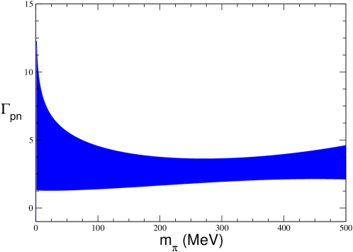
Figure 4: $\Gamma_{pn}$ obtained by letting $C_{\text{mix}}=0$ in (24).

IV Conclusion

The mixed-actions provide us with a powerful tool in lattice simulations because they enable one to use different type of fermions in the valence and sea sectors. In particular, current lattice calcualtions using Ginsparg-Wilson valence quarks in staggered sea quarks can reach the dynamical pion masses as low as $300{\text{MeV}}$.

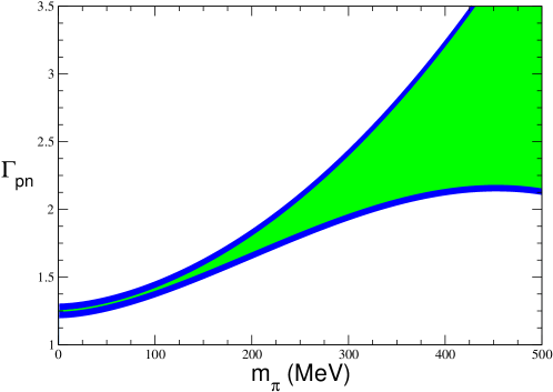
Figure 5: The blue band is the $\Gamma_{pn}$ obtained by letting $C_{\text{mix}}=C_{3}+C_{4}=0$. The green band represents the $\Gamma_{pn}$ with $a=0$.

In this paper, we have calculated the $pn$ matrix element of the axial-vector current up to $O(\epsilon^{3})$ order using the mixed-action of Ginsparg-Wilson valence quarks in staggered sea quarks. Further, we have detailed the lattice spacing artifacts for this matrix element. To $O(\epsilon^{3})$, we found that the $pn$ axial-current matrix element depends on the lattice spacing via three parameters, namely, $C_{{\text{mix}}}$, $C_{3}+C_{4}$ and finally a new low energy constant $C^{\prime}$. The low energy constant $C_{{\text{mix}}}$ affects the masses of mesons made from a Ginsparg-Wilson quark and a staggered quark. Its physical value can be fixed either from mixed meson masses or the pion charge radius bct:0607 . Further, the combination of parameters $C_{3}+C_{4}$ has been already constrained from staggered meson lattice data Aubin et al. (2004c). The new low energy constant $C^{\prime}$, on the other hand, can be evaluated from the lattice simulations of determining the nucleon axial charge Blum:2004 ; Khan:2005 ; Edward:2005 . However, as has been already demonstrated in bct:0607 , the continuum extrapolation with only one lattice spacing available will lead to a large amount of uncertainty in the physical values of the associated low energy constants. Ideally, this low energy constant $C^{\prime}$ will be more accurately determined if a variety of lattice spacings in the lattice simulations are available.

Lastly, since the finite volume effects are small at the scale of dynamical quark masses and the box size available in today’s simulations as indicated in s&m:2004 ; Edward:2005 , the formulas given here should be sufficient for the comparisons between the predictions from $\chi$PT and the results from numerical simulations.

V Appendix

In this Appendix, we list the functions needed in our calculations:

$$\qquad\qquad R_{1}(m,\mu)=\frac{1}{16\pi^{2}}m^{2}\log\Big{(}\frac{m^{2}}{\mu^{2}}\Big{)}\,,\qquad\qquad\$$

(26)

$$K_{1}(m,\Delta,\mu) = \,-\,\frac{1}{2}\frac{1}{16\pi^{2}}\Delta^{2}\log\Big{(}\frac{\mu^{2}}{4\Delta^{2}}\Big{)}\,+\,\frac{3}{4}\frac{1}{16\pi^{2}}\Bigg{(}\Big{(}m^{2}-{2\over 3}\Delta^{2}\Big{)}\log\Big{(}{m^{2}\over\mu^{2}}\Big{)}$$ (27)

$$\quad\,+\,{2\over 3}\Delta\sqrt{\Delta^{2}-m^{2}}\log\Big{(}{\Delta-\sqrt{\Delta^{2}-m^{2}+i\epsilon}\over\Delta+\sqrt{\Delta^{2}-m^{2}+i\epsilon}}\Big{)}$$

$$\quad\,+\,{2\over 3}{m^{2}\over\Delta}\Big{(}\ \pi m-\sqrt{\Delta^{2}-m^{2}}\log\Big{(}{\Delta-\sqrt{\Delta^{2}-m^{2}+i\epsilon}\over\Delta+\sqrt{\Delta^{2}-m^{2}+i\epsilon}}\Big{)}\Big{)}\Bigg{)}\,.$$

$$J_{1}(m,\Delta,\mu) = \,-\,\frac{3}{2}\frac{1}{16\pi^{2}}\Delta^{2}\log\Big{(}\frac{\mu^{2}}{4\Delta^{2}}\Big{)}\,+\,\frac{3}{4}\frac{1}{16\pi^{2}}\Bigg{(}\Big{(}m^{2}-2\Delta^{2}\Big{)}\log\Big{(}{m^{2}\over\mu^{2}}\Big{)}\quad\qquad$$ (28)

$$\quad\,+\,2\Delta\sqrt{\Delta^{2}-m^{2}}\log\Big{(}{\Delta-\sqrt{\Delta^{2}-m^{2}+i\epsilon}\over\Delta+\sqrt{\Delta^{2}-m^{2}+i\epsilon}}\Big{)}\Bigg{)}\,.$$

References

- Aubin et al. (2004c) C. Aubin et al. (MILC), Phys. Rev. D70, 114501 (2004c), eprint hep-lat/0407028.
- Aubin et al. (2005a) C. Aubin et al. (Fermilab Lattice), Phys. Rev. Lett. 94, 011601 (2005a), eprint hep-ph/0408306.
- (3) Silas R. Beane et al., Phys. Rev. D73, 054503 (2005), hep-lat/0506013.
- (4) R. G. Edward et al., PoS LAT2005, 056 (2005), hep-lat/0509185
- (5) R. G. Edward et al., Phys. Rev. Lett 96, 052001 (2006), hep-lat/0510062.
- (6) Silas R. Beane et al., hep-lat/0604013.
- (7) Silas R. Beane et al., hep-lat/0605014.
- (8) C. Alexandrou et al., Phys. Rev. Lett. 98, 052003 (2007), hep-lat/0607030
- (9) Silas R. Beane et al., Phys. Rev. D74, 114503 (2006), hep-lat/0607036.
- (10) R. G. Edward et al., hep-lat/0610007.
- (11) Silas R. Beane et al., hep-lat/0612026.
- Bernard et al. (2001) C. W. Bernard et al., Phys. Rev. D64, 054506 (2001), eprint hep-lat/0104002.
- (13) K. Symanzik, Nucl. Phys. B226, 187 (1983).
- (14) K. Symanzik, Nucl. Phys. B226, 205 (1983).
- Bar et al. (2003) O. Bar, G. Rupak, and N. Shoresh, Phys. Rev. D67, 114505 (2003), eprint hep-lat/0210050.
- Bar et al. (2004) O. Bar, G. Rupak, and N. Shoresh, Phys. Rev. D70, 034508 (2004), eprint hep-lat/0306021.
- (17) Silas R. Beane and Martin J. Savage, Phys. Rev. D68, 114502 (2003), hep-lat/0306036.
- (18) B. C. Tiburzi, Nucl. Phys. A761, 232-258 (2005), hep-lat/0501020.
- (19) O. Bar, C. Bernard, G. Rupak, and N. Shoresh, Phys. Rev. D72, 054502 (2005), hep-lat/0503009.
- (20) B. C. Tiburzi, Phys. Rev. D72, 094501 (2005), hep-lat/0508019.
- (21) W.-M. Yao et al., Journal of Physics G 33, 1 (2006).
- (22) E. Jenkins and A. V. Manohar, Phys. Lett. B255, 558 (1991).
- (23) E. Jenkins and A. V. Manohar, Phys. Lett. B259, 353 (1991).
- (24) T. Blum et al., Phys. Rev. D69, 074502 (2004), hep-lat/0007038.
- (25) A. A. Khan et al., Nucl. Phys. Proc. Suppl. 140, 408 (2005), hep-lat/0409161.
- (26) B. Borasoy, Phys. Rev. D59, 054021 (1999), hep-ph/9811411.
- (27) S.-L. Zhu et al., Phys. Rev. D63, 034002 (2001), hep-ph/0008140.
- (28) Silas R. Beane and Martin Savage, Nucl. Phys. A709, 319-344 (2002), hep-lat/0203003.
- (29) Silas R. Beane and Martin J. Savage, Phys. Rev. D70, 074029 (2004), hep-ph/0404131.
- (30) R. L. Jaffe, Phys. Lett. B529, 105 (2002).
- (31) T. D. Cohen, Phys. Lett. B529, 50 (2002).
- Sharpe and Singleton (1998) S. R. Sharpe and J. Singleton, Robert, Phys. Rev. D58, 074501 (1998), eprint hep-lat/9804028.
- Lee and Sharpe (1999) W.-J. Lee and S. R. Sharpe, Phys. Rev. D60, 114503 (1999), eprint hep-lat/9905023.
- Rupak and Shoresh (2002) G. Rupak and N. Shoresh, Phys. Rev. D66, 054503 (2002), eprint hep-lat/0201019.
- Aubin and Bernard (2003a) C. Aubin and C. Bernard, Phys. Rev. D68, 034014 (2003a), eprint hep-lat/0304014.
- Aubin and Bernard (2003b) C. Aubin and C. Bernard, Phys. Rev. D68, 074011 (2003b), eprint hep-lat/0306026.
- (37) S. R. Sharpe and R. S. Van de Water, Phys. Rev. D71, 114505 (2005), hep-lat/0409018.
- Sharpe and Shoresh (2001) S. R. Sharpe and N. Shoresh, Phys. Rev. D64, 114510 (2001), eprint [http://arXiv.org/abs]hep-lat/0108003.
- (39) M. J. Savage, Nucl. Phys. A700, 359 (2002), hep-lat/0107038.
- (40) J. N. Labrenz and S. R. Sharpe, Phys. Rev. D54, 4595 (1996), hep-lat/9605034.
- (41) B. C. Tiburzi, Phys. Rev. D71, 054504 (2005), hep-lat/0412025.
- (42) B. C. Tiburzi, Phys. Lett. B617, 40-48 (2005), hep-lat/0504002.
- (43) T. B. Bunton et al., Phys. Rev. D74, 034514 (2006); Erratum-ibid. D74, 099902 (2006), hep-lat/0607001.
- (44) Maarten Golterman et al., Phys. Rev. D71, 114508 (2005), hep-lat/0504013.