Infrared properties of propagators in Landau-gauge pure Yang-Mills theory at finite temperature

Abstract

The finite-temperature behavior of gluon and of Faddeev-Popov-ghost propagators is investigated for pure $SU(2)$ Yang-Mills theory in Landau gauge. We present nonperturbative results, obtained using lattice simulations and Dyson-Schwinger equations. Possible limitations of these two approaches, such as finite-volume effects and truncation artifacts, are extensively discussed. Both methods suggest a very different temperature dependence for the magnetic sector when compared to the electric one. In particular, a clear thermodynamic transition seems to affect only the electric sector. These results imply in particular the confinement of transverse gluons at all temperatures and they can be understood inside the framework of the so-called Gribov-Zwanziger scenario of confinement.

I Introduction

Thermodynamic observables, such as the free energy, show a thermodynamic transition in Yang-Mills theory at a finite temperature $T_{c}$ Karsch:2001cy ; Karsch:2003jg . This phase transition separates a low-temperature phase — which is expected to be highly non-perturbative and characterized by quark and gluon confinement — from a (in principle) perturbative high-temperature phase, where color charges should be deconfined. Indeed, due to asymptotic freedom, the running coupling constant $g(T)$ vanishes with increasing temperature LeBellac and the quark-gluon plasma can be viewed as a weakly-coupled system. At the same time, across the phase transition, the long-distance potential between fundamental test-charges changes from a linearly-rising confining potential to an essentially flat one Kaczmarek:2004gv , i.e. the (temporal) string tension is zero at high temperature.

On the other hand, non-perturbative phenomena have to be expected even for an arbitrarily small coupling at the renormalization scale Haag:1992hx . In particular, several studies have already pointed out that non-perturbative effects should be present in Yang-Mills theory at any temperature, i.e. the high-temperature phase should also be highly non-trivial. For example, it is well-known that the magnetic sector is affected by strong non-perturbative infrared (IR) problems Linde:1980ts ; Maas:2005ym . Moreover, at finite temperature, the spatial string tension is non-vanishing Bali . Finally, the formal infinite-temperature limit of the theory, i.e. the 3-dimensional reduced theory Maas:2005ym ; Appelquist:1981vg , is still a confining theory Maas:2005ym ; 3d ; Zwanziger ; Cucchieri:2004mf ; Maas:2004se . Thus, a clear description of Yang-Mills theory as a function of the temperature $T$ is still lacking and the fate of confinement at large T is still an open question. In particular, one should reconcile the confining properties of the dimensionally-reduced theory with the vanishing of the conventional string tension at large temperature.

In order to make contact with the continuum formulation of $SU(N_{c})$ Yang-Mills theory, it is necessary to consider quantities living either in the $su(N_{c})$ algebra or in the continuum gauge group $SU(N_{c})/Z_{N}$ O'Raifeartaigh:1986vq . This clearly limits the usefulness of center observables such as the Polyakov line, often employed in lattice simulations and in effective theories. On the other hand, propagators of the elementary degrees of freedom of the theory, such as gluon and ghost fields, fulfill the above condition and provide access to non-perturbative aspects of the theory Alkofer:2000wg ; Fischer:2006ub .

In Landau gauge, at zero temperature, the framework of the Gribov-Zwanziger Zwanziger ; Gribov and of the Kugo-Ojima Kugo scenarios provides a basis for understanding the confinement mechanism in Yang-Mills theory. In particular, these scenarios predict that the ghost propagator should be IR enhanced, compared to the propagator of a massless particle. At the same time, the gluon propagator should vanish in the IR limit. These predictions are supported by results obtained using different methods Alkofer:2000wg ; Fischer:2006ub ; Zwanziger ; vonSmekal ; Watson:2001yv ; Cucchieri:2001za ; Gies ; Lerche:2002ep ; Bloch:2003sk ; Schleifenbaum:2004id ; Alkofer ; Ilgenfritz:2006gp ; Ilgenfritz:2006he ; Sternbeck:2005tk ; Cucchieri:2006xi . In addition, several calculations indicate that the predictions are also (at least partially) valid in the high-temperature phase Maas:2005ym ; Cucchieri ; Zahed:1999tg ; Maas:2005hs and in the infinite-temperature limit Maas:2005ym ; Zwanziger ; Cucchieri:2004mf ; Maas:2004se ; Cucchieri ; Schleifenbaum:2004id ; Cucchieri:2006xi ; Cucchieri:1999sz ; Cucchieri:2003di ; Cucchieri:2006tf .

Here we evaluate gluon and ghost propagators for the $SU(2)$ case using Landau gauge, extending earlier numerical studies that focused on the high-temperature phase Cucchieri and on the infinite-temperature limit Cucchieri ; Cucchieri:1999sz ; Cucchieri:2003di ; Cucchieri:2006tf . We present nonperturbative results, obtained using lattice simulations and Dyson-Schwinger equations (DSEs). In Section II we present a short review of the Lorentz structure for the Landau-gauge gluon and Faddeev-Popov-ghost propagators at finite temperature. Results using lattice gauge theory for these two propagators at various temperatures, both below and above the thermodynamic transition, will be reported in Section III. In that section we also discuss the influence of finite-volume effects on the numerical results. In Section IV the same propagators are studied in continuum space-time using DSEs, which allows us to consider the limit of vanishing momentum $p\to 0$. Let us recall Zwanziger that imposing the minimal Landau gauge condition, i.e. restricting to the Gribov region, does not modify the DSEs, even though it provides supplementary conditions for their solution. We believe that the simultaneous use of these two nonperturbative methods — lattice simulations and DSEs — allows a better understanding of our results and of their physical implications. A possible interpretation of the results from lattice and from DSEs is presented in Section V. The main components of this interpretation are a spatial/magnetic sector, which is essentially unaffected by temperature and by the thermodynamic transition, and a temporal/electric sector, which does show a sensitivity to the transition. Let us stress that the results from DSEs suggest that the difference between the two sectors occurs for any non-zero temperature and not only above the phase transition. In particular, the Gribov-Zwanziger and Kugo-Ojima confinement mechanisms remain qualitatively unaltered in the magnetic sector when the temperature is turned on. Finally, we present our conclusions in Section VI. Some observations about the use of asymmetric lattices in numerical simulations are reported in Appendix A. Analytic and numerical details of the DSE analysis, presented in Section IV, are collected in Appendices B–D.

Preliminary results have been presented in Maas:2006qw .

II Propagators at finite temperature

At finite temperature, the Euclidean symmetry is manifestly broken by the thermal heat bath. As a consequence, the propagator of the gluon, which is a vector particle, can no longer be described by a single tensor structure. Instead, one can consider the decomposition Kapusta:tk

$$D_{\mu\nu}^{ab}(p)\,=\,P_{\mu\nu}^{T}(p)\,D_{T}^{ab}(p)\,+\,P_{\mu\nu}^{L}D_{L}^{ab}(p)\;,$$ (1)

where the two tensor structures $P_{\mu\nu}^{T}(p)$ and $P_{\mu\nu}^{L}(p)$ are respectively transverse and longitudinal in the (three-dimensional) spatial sub-space. Of course, in the full 4d space both tensors must be transverse, due to the Landau gauge condition. In terms of the momentum components $p_{\mu}$ we can write (with no summation over repeated indices) Kapusta:tk

$$P_{\mu\nu}^{T}(p) = (1-\delta_{\mu 0})(1-\delta_{\nu 0})\left(\delta_{\mu\nu}-\frac{p_{\mu}p_{\nu}}{\vec{p}^{2}}\right)$$ (2)

$$P_{\mu\nu}^{L}(p) = P_{\mu\nu}(p)\,-\,P_{\mu\nu}^{T}(p)\;.$$ (3)

Clearly, the tensor $P^{T}_{\mu\nu}(p)$ is the transverse projector in the three-dimensional spatial sub-space, while $P^{L}_{\mu\nu}(p)$ is the complement of $P^{T}_{\mu\nu}(p)$ to the four-dimensional Euclidean-invariant transverse projector $P_{\mu\nu}(p)=\delta_{\mu\nu}-p_{\mu}p_{\nu}/p^{2}$. At the same time, the decomposition (1) defines the two independent scalar propagators $D_{T}^{ab}(p)$ and $D_{L}^{ab}(p)$, which are respectively the coefficients of the 3d-transverse and of the 3d-longitudinal projectors. Since one expects a different IR behavior for these two functions, it is not useful to contract the gluon propagator with the usual 4d-transverse projector $P_{\mu\nu}(p)$, i.e. to consider a linear combination of the two scalar functions $D_{T}^{ab}(p)$ and $D_{L}^{ab}(p)$. By contracting the propagator $D_{\mu\nu}^{ab}(p)$ with $P^{T}_{\mu\nu}(p)$ or with $P_{\mu\nu}^{L}(p)$, inserting a unit matrix in color space and using the relation

$$p_{0}\,A_{0}^{a}\,=\,-\sum_{\mu=1}^{3}\,p_{\mu}\,A_{\mu}^{a}\;,$$ (4)

valid in Landau gauge, we find (for non-zero three-momentum ${\vec{p}}$) the relations

$$\!\!\!\!\!\!\!D_{T}(p) = \frac{1}{(d-2)N_{g}}$$ (5)

$$\times <\sum_{\mu=1}^{3}\,A_{\mu}^{a}(p)A_{\mu}^{a}(-p)-\frac{p_{0}^{2}}{{\vec{p}\,}^{2}}\,A_{0}^{a}(p)A_{0}^{a}(-p)>$$

$$\!\!\!\!\!\!\!D_{L}(p) = \frac{1}{N_{g}}\left(1+\frac{p_{0}^{2}}{{\vec{p}\,}^{2}}\right)<A_{0}^{a}(p)A_{0}^{a}(-p)>\;.$$ (6)

Here, $d=4$ is the space-time dimension, $N_{g}=3$ is the number of gluons [i.e. $N_{g}=N^{2}_{c}-1$ in the $SU(N_{c})$ case] and the summation over color indices is implied. Clearly, for $p_{0}=0$ the 3d-transverse propagator $D_{T}(p)$ coincides with the 3d gluon propagator, while the 3d-longitudinal propagator $D_{L}(p)$ can be identified with the propagator of the would-be-Higgs field in the three-dimensionally-reduced theory. Thus, we can associate the 3d-transverse gluon propagator to the so-called magnetic sector and the 3d-longitudinal propagator to the electric sector. Of course, at zero temperature the two scalar propagators coincide, i.e. $D_{T}(p)\,=\,D_{L}(p)\,=\,D(p)$.

Table 1: Data of the configurations considered in our numerical simulations. The three-dimensional case will be discussed in Section III.1. The Setup column will be used in the text to refer to the various numerical setups. The value of the lattice spacing $a$ has been taken from Cucchieri:2003di for the three-dimensional case and from Fingberg:1992ju for the four-dimensional case. Sweeps indicates the number of sweeps between two consecutive gauge-fixed measurements. The temperature has been evaluated using Eq. (8). In the column Method we indicate a reference where numerical details (including error determination, etc.) are discussed for that particular set of data. With the symbols ⁺ and ^∗ we indicate that (respectively) only the gluon or only the ghost propagator has been considered. Note that only the results corresponding to the Setups 16, 17, 19, and 20 have already been published. Finally, in the Setup 6 we found one “exceptional” configuration that induced very large statistical fluctuations on the results. Thus, in this case, we needed a much larger statistics in order to acquire the same level of accuracy obtained in the other cases.

Setup	$N^{4}$, $N_{t}\times N_{s}^{3}$ or $N^{3}$	$\beta$	$a^{-1}$ [GeV]	Configurations	Sweeps	$T$ [MeV]	$V_{s}^{1/3}$ [fm]	Method
1	$12^{4}$	2.3	1.193	426	40	0	1.98	Cucchieri:2006tf +
2	$16^{4}$	2.3	1.193	424	45	0	2.64	Cucchieri:2006tf +
3	$20^{4}$	2.3	1.193	405	50	0	3.30	Cucchieri:2006tf +
4	$32^{4}$	2.3	1.193	30	320	0	5.28	Bloch:2003sk ∗
5	$10\times 14^{3}$	2.3	1.193	401	40	119	2.31	Cucchieri:2006tf
6	$10\times 20^{3}$	2.3	1.193	1426	45	119	3.30	Cucchieri:2006tf
7	$10\times 26^{3}$	2.3	1.193	405	50	119	4.29	Cucchieri:2006tf
8	$4\times 20^{3}$	2.3	1.193	444	40	298	3.30	Cucchieri:2006tf
9	$4\times 26^{3}$	2.3	1.193	405	45	298	4.29	Cucchieri:2006tf
10	$4\times 34^{3}$	2.3	1.193	405	50	298	5.61	Cucchieri:2006tf
11	$3\times 28^{3}$	2.4	1.651	429	50	550	3.34	Cucchieri:2006tf
12	$4\times 40^{3}$	2.5	2.309	360	50	577	3.41	Cucchieri:2006tf
13	$2\times 20^{3}$	2.3	1.193	437	40	597	3.30	Cucchieri:2006tf
14	$2\times 32^{3}$	2.3	1.193	410	45	597	5.28	Cucchieri:2006tf
15	$2\times 42^{3}$	2.3	1.193	400	50	597	6.93	Cucchieri:2006tf
16	$20^{3}$	4.2	1.136	6161	40	0	3.47	Cucchieri:2006tf
17	$30^{3}$	4.2	1.136	10229	45	0	5.20	Cucchieri:2006tf
18	$40^{3}$	4.2	1.136	3306	50	0	6.94	Cucchieri:2006tf
19	$80^{3}$	4.2	1.136	200	200	0	13.9	Cucchieri:2003di +, Cucchieri:2006za ∗
20	$140^{3}$	4.2	1.136	30	250	0	24.3	Cucchieri:2003di +

As for the ghost propagator $D_{G}(p)$, since it is a scalar function, no additional tensor structures arise in this case.

A second consequence of considering a theory at finite temperature is that the propagators depend separately on the energy $p_{0}$ and on the spatial three-momentum $|\vec{p}|$. Moreover, the energy is always discrete, i.e. $p_{0}=2\pi Tn$ with $n$ integer. Of course, in studying the IR properties of the theory, we are mainly interested in the zero (or soft) modes $p_{0}=0$. The other (hard) modes ($p_{0}\neq 0$) have an effective thermal mass of $2\pi Tn$ and seem to behave like massive particles Maas:2005ym ; Maas:2005hs ; Kapusta:tk ; Blaizot:2001nr .

Let us stress that these observations apply both to the lattice and to the continuum formulations of Yang-Mills theory. In the lattice case one also has to consider the definition of the gluon field

$$A_{\mu}(x)\,=\,\frac{1}{2i}\left[\,U_{\mu}(x)\,-\,U_{\mu}^{\dagger}(x)\,\right]_{traceless}$$ (7)

as a function of the link variables $U_{\mu}(x)$, which is based on the expansion $U_{\mu}(x)\,\approx\,1\!\!\!\bot\,+\,ig_{0}aA_{\mu}(x)$ . Hence, in the high-temperature (symmetry-broken) phase, one should consider only configurations for which the trace of the Polyakov loop has a positive value when averaged over the lattice Cucchieri ; Karsch:1994xh .

III Lattice results

The propagators of the gluon and of the Faddeev-Popov ghost have been numerically evaluated using the methods described in Refs. Cucchieri:2006tf ; Bloch:2003sk ; Cucchieri:2003di ; Cucchieri:2006za . Details can also be found in Table 1. Finite temperature has been introduced according to the standard procedure of reducing the extent of the time direction compared to the spatial ones Rothe:1997kp . We consider $N_{t}$ lattice sites along the temporal direction and $N_{s}$ sites along the spatial direction with $N_{s}\gg N_{t}$. After taking the infinite-spatial-volume limit $V_{s}=N_{s}^{3}\to\infty$ , the continuum limit is given by $N_{t}\to\infty$ and $a\to 0$, keeping the product $aN_{t}$ fixed. This yields a temperature

$$T\,=\,\frac{1}{aN_{t}}\;.$$ (8)

In the following, we first consider the symmetric three-dimensional case, discussing finite-volume effects in detail. We then move on to the four-dimensional case and discuss the effects of finite temperature.

III.1 Finite-volume effects

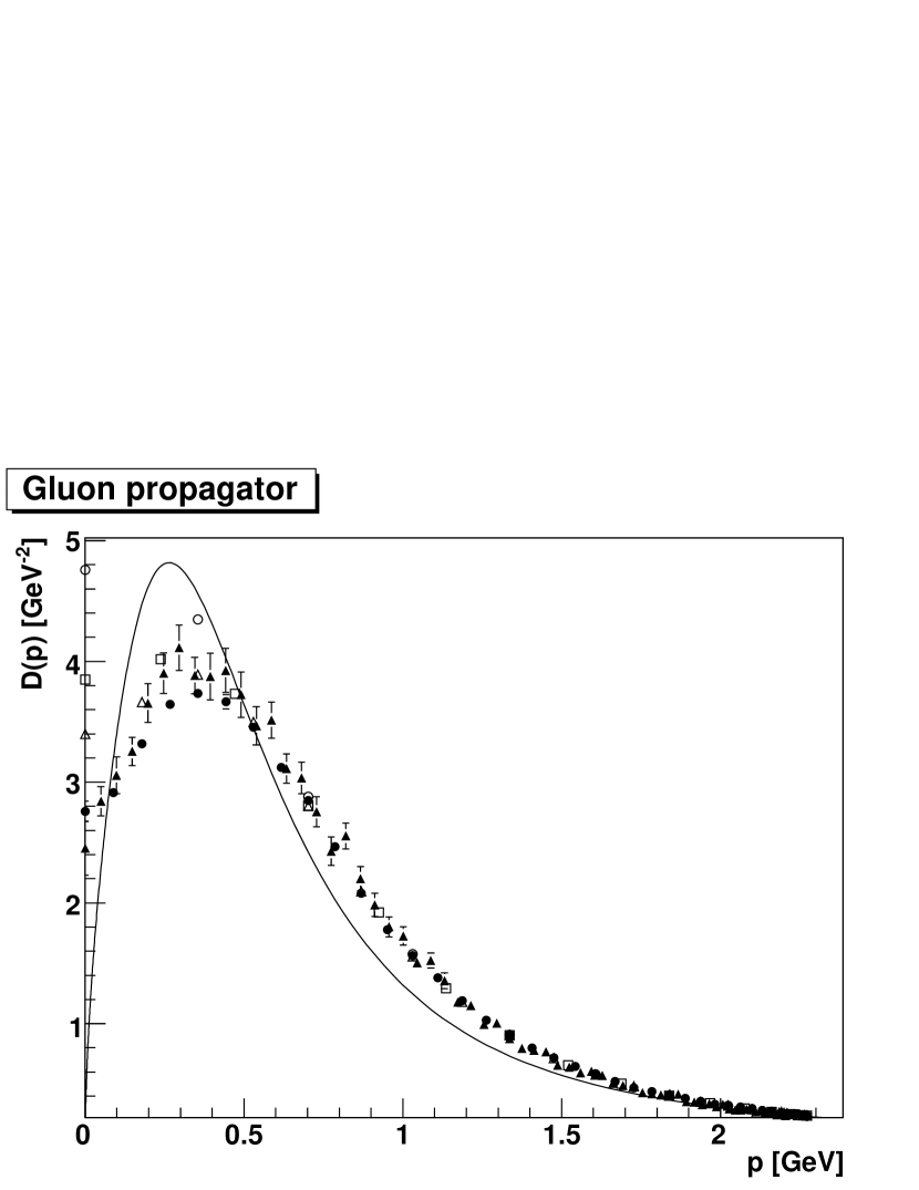
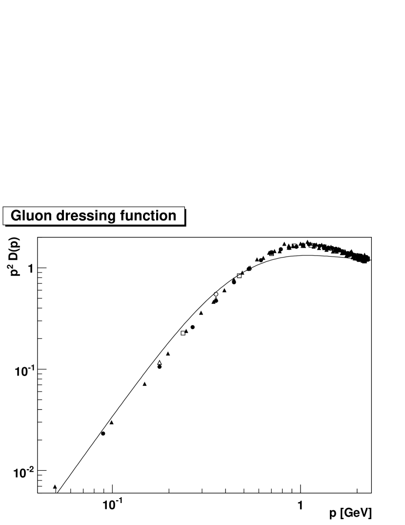
Figure 1: The gluon propagator $D(p)$ (top) and dressing function $p^{2}D(p)$ (bottom) as a function of the momentum $p$ for various volumes in three dimensions. Open circles, open squares, open triangles, full circles and full triangles correspond to Setups 16 ($V=20^{3}$), 17 ($V=30^{3}$), 18 ($V=40^{3}$), 19 ($V=80^{3}$) and 20 ($V=140^{3}$), respectively. The solid line is the result from Dyson-Schwinger calculations Maas:2004se , yielding a gluon propagator suppressed as $p^{0.59}$ in the IR limit.

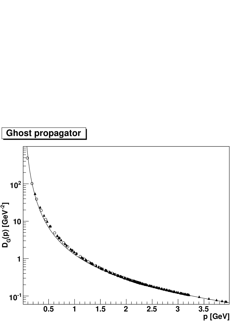
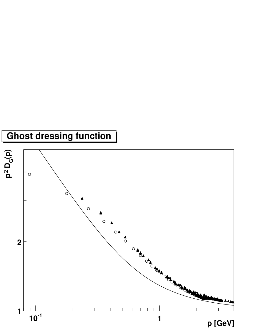
Figure 2: The ghost propagator $D_{G}(p)$ (top) and the dressing function $p^{2}D_{G}(p)$ (bottom) as a function of the momentum $p$ for two different volumes in three dimensions. Full triangles and open circles correspond to Setups 17 ($V=30^{3}$) and 19 ($V=80^{3}$), respectively. The solid line is the result from Dyson-Schwinger calculations Maas:2004se , yielding a ghost propagator enhanced as $p^{-2.8}$ in the IR limit.

Figure 3: The effective coupling $p^{5}\,D_{G}^{2}(p)\,D(p)$ as a function of the momentum $p$ for Setups 17 (open squares, $V=30^{3}$) and 19 (full triangles, $V=80^{3}$). The solid line is the result from the same Dyson-Schwinger calculations Maas:2004se reported in Figs. 1 and 2.

Before considering the finite-temperature dependence of the propagators, it is worthwhile to discuss the effects of finite volume on their IR behavior. Clearly, a finite volume $V$ affects all processes with a correlation length $\xi$ of the order of (or larger than) $V^{1/d}$. [In the finite-temperature case one can expect finite-volume effects when $\xi\gtrsim V_{s}^{1/(d-1)}$, where $V_{s}$ is the spatial volume.] Since confinement is induced by an infinite correlation length Alkofer:2000wg , finite-volume effects are likely to be observed in the numerical evaluation of gluon and ghost propagators. These effects should be considered when comparing the numerical data to the predictions of the Gribov-Zwanziger and of the Kugo-Ojima confinement scenarios. Let us recall that several calculations in the continuum, e.g. using DSEs Zwanziger ; Alkofer:2000wg ; Fischer:2006ub ; vonSmekal or the renormalization group Gies , are in favor of these scenarios and confirm their predictions. In addition, using DSEs one can also study (in the continuum) the consequences of a finite volume on these propagators. In particular, it has been found fischer that in a finite volume the gluon propagator is suppressed at small momenta and finite at zero momentum, while the ghost propagator is IR enhanced. These results are in qualitative agreement with the findings using lattice calculations Bloch:2003sk ; Ilgenfritz:2006gp ; Ilgenfritz:2006he ; Silva . Moreover, using DSEs it can be argued fischer that an IR-finite gluon propagator is indeed an artifact of the finite volume and that one obtains a null propagator at $p=0$ when the infinite-volume limit is considered. On the lattice the situation is clearly more complicated. Even in the case of a power-dependence of the type $D(0)\propto 1/V^{b}$, it can be very difficult Cucchieri:2003di to perform simulations with sufficiently large values of the physical lattice volume $V$ so that one can really control the extrapolation to infinite volume. This is in fact the case and up to now there is not yet any convincing result on a (symmetric) four-dimensional lattice showing an IR-vanishing gluon propagator $D(p)$. The situation is actually even worse than this. Indeed, in order to see an IR-suppressed propagator one should obtain that $D(p)$ has a maximum for some value of $p\neq 0$. Up to now this has not been obtained in the Landau 4d case (using symmetric lattices), even when considering very large lattices (see Fig. 10 in Cucchieri:2006xi and Fig. 3 in Ilgenfritz:2006he ). There are, however, evidences of a suppressed gluon propagator when considering 4d asymmetric lattices Silva , even though in this case it is difficult to extract quantitative information from the data Cucchieri:2006za ; Ilgenfritz:2006gp . Also, a suppressed gluon propagator at small momenta can be obtained in the 4d case when simulations are done in the strong-coupling regime Cucchieri:1997fy . Finally, a suppressed gluon propagator has recently been obtained (using symmetric lattices and $\beta$ values in the scaling region) for a Landau-like gauge condition Cucchieri:2007uj , confirming that the difficulties in finding a similar IR-suppressed gluon propagator in Landau gauge are probably related to finite-size effects.

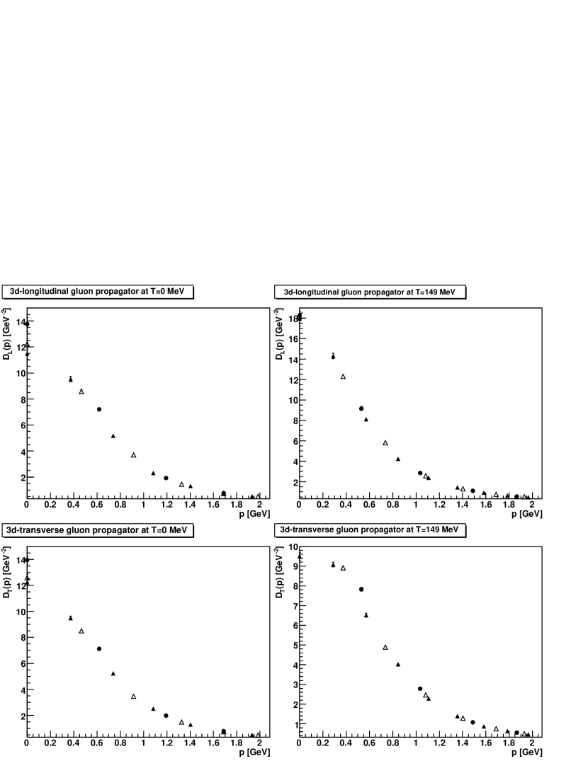
Figure 4: The volume dependence of the gluon propagators in the low-temperature phase. The top panels show the 3d-longitudinal propagator while in the bottom panels we report results for the 3d-transverse propagator. The left panels show the results at zero temperature ($N_{s}=N_{t}$) and the right panels at $T\approx 119$ MeV ($N_{t}=10$), well inside the low-temperature phase. We always compare results obtained using three different physical volumes. The smallest volumes (Setups 1 and 5) are indicated with full circles, the middle-size volumes (Setups 2 and 6) are represented by open triangles and the largest volumes (Setups 3 and 7) are indicated by full triangles. Momenta are aligned along the $x$ axis.

Numerically, it is clearly easier to consider first the three-dimensional case, since one can then use much larger lattice sides. Moreover, the Gribov-Zwanziger scenario can be applied to three dimensions Zwanziger:1990by — as also supported by numerical studies Cucchieri ; Cucchieri:1999sz ; Cucchieri:2006tf ; Cucchieri:2003di and by calculations using DSEs Zwanziger ; Maas:2004se — and the IR suppression of the gluon propagator is expected to be stronger than in the 4d case (i.e. the IR exponent is larger in the 3d case). Finally, since the theory is finite, renormalization issues do not obscure the interpretation of the results. Let us recall that various lattice calculations have been performed in the 3d case, both for the propagators Cucchieri ; Cucchieri:1999sz ; Cucchieri:2006tf ; Cucchieri:2003di and for the 3-point vertices Cucchieri:2006tf . These results support the assumptions usually made in DSE calculations Maas:2004se .

We now consider symmetric lattices in the 3d case (see run parameters at the bottom of Table 1). These can be interpreted as lattices at $T=0$ in 3d or as lattices at $T=\infty$, simulating the dimensionally-reduced theory (without the Higgs field). We compare the numerical data to Dyson-Schwinger calculations Maas:2004se . In Fig.  1 we present results in the 3d case for the gluon propagator using lattice simulations and DSE calculations. Considering the lattice data on the larger lattices, there is a clear maximum at $p_{max}\approx 400$ MeV. Moreover, as the lattice volume increases, the IR suppression becomes stronger. However, even using very large volumes (i.e. $V=140^{3}$ Cucchieri:2003di ), only few momenta are available in the interval $[0,p_{max}]$. The comparison to the DSE solution (for infinite volume) shows qualitative agreement. Concerning the gluon dressing function $p^{2}D(p)$, it is found that lattice results exhibit a power-law behavior for momenta below $400-500$ MeV. The result is very similar to the DSE solution, albeit differing by a constant factor. Of course, when considering the dressing function $p^{2}D(p)$, the factor $p^{2}$ is dominant in the IR limit and the agreement between lattice and DSE results looks better. Also note that the pre-factor of the power-law obtained in DSE studies is sensitive to the approximations performed Maas:2004se .

Figure 5: The volume dependence of the gluon propagators in the high-temperature phase. The top panels show the 3d-longitudinal propagator while in the bottom panels we report results for the 3d-transverse propagator. The left panels show the results at $T\approx 298$ MeV ($N_{t}=4$), slightly above the thermodynamic transition, and the right panels at $T\approx 597$ MeV ($N_{t}=2$), well inside the high-temperature phase. We always compare results obtained using three different physical volumes. The smallest volumes (Setups 8 and 13) are indicated with full circles, the middle-size volumes (Setups 9 and 14) are represented by open triangles and the largest volumes (Setups 10 and 15) are indicated by full triangles. Momenta are aligned along the $x$ axis.

Results for the ghost propagator $D_{G}(p)$ and the dressing function $p^{2}D_{G}(p)$ are reported in Fig.  2. In this case there are no evident finite-volume effects in the lattice data for $D_{G}(p)$, even though such effects are visible at small momenta when considering the dressing function $p^{2}D_{G}(p)$. In particular, the dressing function shows a reduced IR divergence for the largest lattice at small momenta $p$. On the other hand, one should recall that, for a relatively small statistics, the so-called “exceptional configurations” are probably not adequately sampled and that they contribute significantly to the IR enhancement of $D_{G}(p)$, i.e. this IR enhancement could be underestimated Sternbeck:2005tk ; Cucchieri:2006tf . When considering the comparison to DSE results, we see that agreement is again at the qualitative level (see in particular the dressing function in the bottom figure). Indeed, the lattice data show a weaker divergence than the one obtained using DSE calculations. As said above, this could be related to an insufficient statistics for the ghost propagator when large lattice volumes are used.

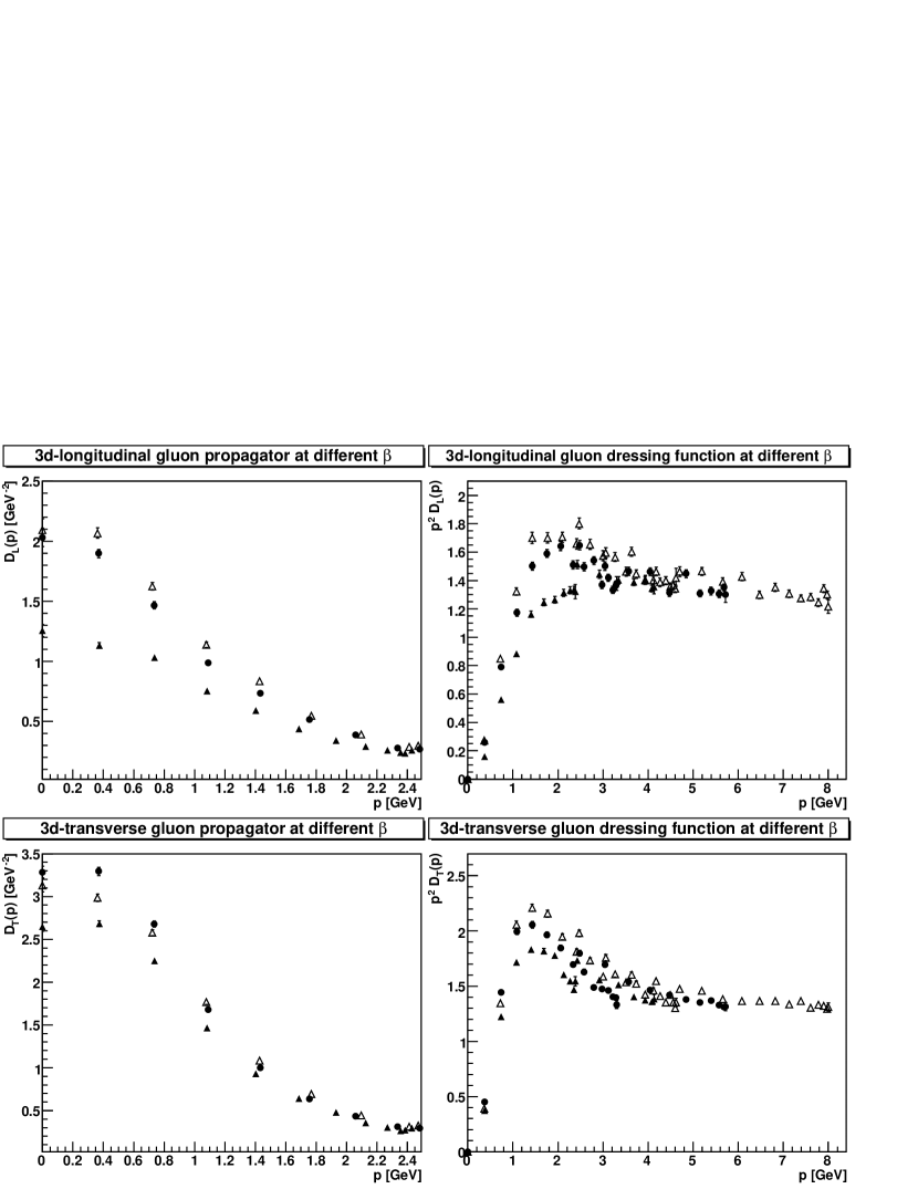
Figure 6: The $\beta$ dependence of the gluon propagators for a physical spatial volume $V_{s}$ of approximately $(3.35$ fm$)^{3}$ and temperature $T\approx 575MeV$, using three different lattice setups. We report data for the 3d-longitudinal propagator in the top-left panel, for the 3d-longitudinal dressing function in the top-right panel, for the 3d-transverse propagator in the bottom-left panel and for the 3d-transverse dressing function in the bottom-right panel. We represent with full triangles data at $\beta=2.3$ (Setup 13), with full circles data obtained at $\beta=2.4$ (Setup 11) and with open triangles results for $\beta=2.5$ (Setup 12). Momenta below approximately 2.4 GeV are considered along the $x$-axis, larger momenta are along the 3d-spatial diagonal.

Finally, one can consider the effective coupling defined to be proportional to $p^{5}\,D_{G}^{2}(p)\,D(p)$, for which DSEs predict a constant limit at zero momentum. The comparison of lattice data and DSE results is made in Fig.  3. It is clear that the asymptotic (constant) regime is reached in the Dyson-Schwinger result only for momenta of the order of 200 MeV. For the lattice data, when $V=30^{3}$, we do not have any point in the range $[0,200]$ MeV and it is difficult to say what one could find in the $p=0$ limit. On the other hand, in the case of the larger lattice ($V=80^{3}$), one sees a coupling decreasing when $p$ is smaller than about $p_{max}\approx 400$ MeV. It thus seems that the two approaches differ qualitatively in the deep IR limit. Nevertheless, it is interesting to note that the maximum of the data for the larger lattice is obtained for the momentum $p=p_{max}\approx 400$ MeV, where also the gluon propagator reaches its maximum value. Thus, a possible interpretation Cucchieri:2006xi ; fischer is that finite-size effects are different for the two propagators and one might see an IR-finite effective coupling only in the infinite-volume limit. In other words, since the prediction from DSE studies is based on the relation $a_{D}-2a_{G}=(4-d)/2$ Zwanziger ; Lerche:2002ep , one can imagine that the true values for the exponents $a_{D}$ and $a_{G}$ are obtained only in the infinite-volume limit and that at finite volume the above relation does not need to be satisfied.

Let us note that Dyson-Schwinger studies find that the expected power-law behaviors for the propagators (in 3d as well as in 4d) start to appear only for momenta smaller than some energy-scale $\Lambda_{I}\lesssim 200$ MeV fischer . Also, one should consider with caution lattice results at the smallest non-zero momentum $\,2/a\sin(\pi/N)\approx 2\pi/(aN)$, i.e. when the quantities considered may “feel” the boundaries. Thus, one should try to extract the IR behavior of the propagators only using data in the range

$$\frac{2}{a}\sin\left(\frac{\pi}{N}\right)\ll p\lesssim\Lambda_{I}.$$ (9)

With a lattice spacing $a$ of order of 1 GeV^-1 one consequently needs $N\gg 50$. Present simulations have access to this region only in the three-dimensional case. In the four-dimensional case the situation is more complicated and, in particular, since the IR suppression of the 4d gluon propagator is predicted to be weaker than in three dimensions ($p^{0.38}$ instead of $p^{0.59}$) Zwanziger ; Lerche:2002ep , one probably needs even larger lattice sides than in the 3d case, making these computational studies very demanding. Looking at the results obtained in the 3d case and considering the data obtained with the largest 4d lattices available Cucchieri:2006xi ; Ilgenfritz:2006he , one can argue that volumes larger by a factor of 10 (i.e. a factor of about 2 in lattice side) are probably necessary in order to see a decreasing gluon propagator also in the 4d case. On the other hand, for the ghost propagator and with the available lattice sides, the IR-enhancement is clearly observed Bloch:2003sk ; Ilgenfritz:2006he ; Silva ; Ilgenfritz:2006gp . even though the value obtained numerically for the IR exponent $a_{G}$ is usually smaller than the DSE result Zwanziger ; Lerche:2002ep .

III.2 Finite temperature

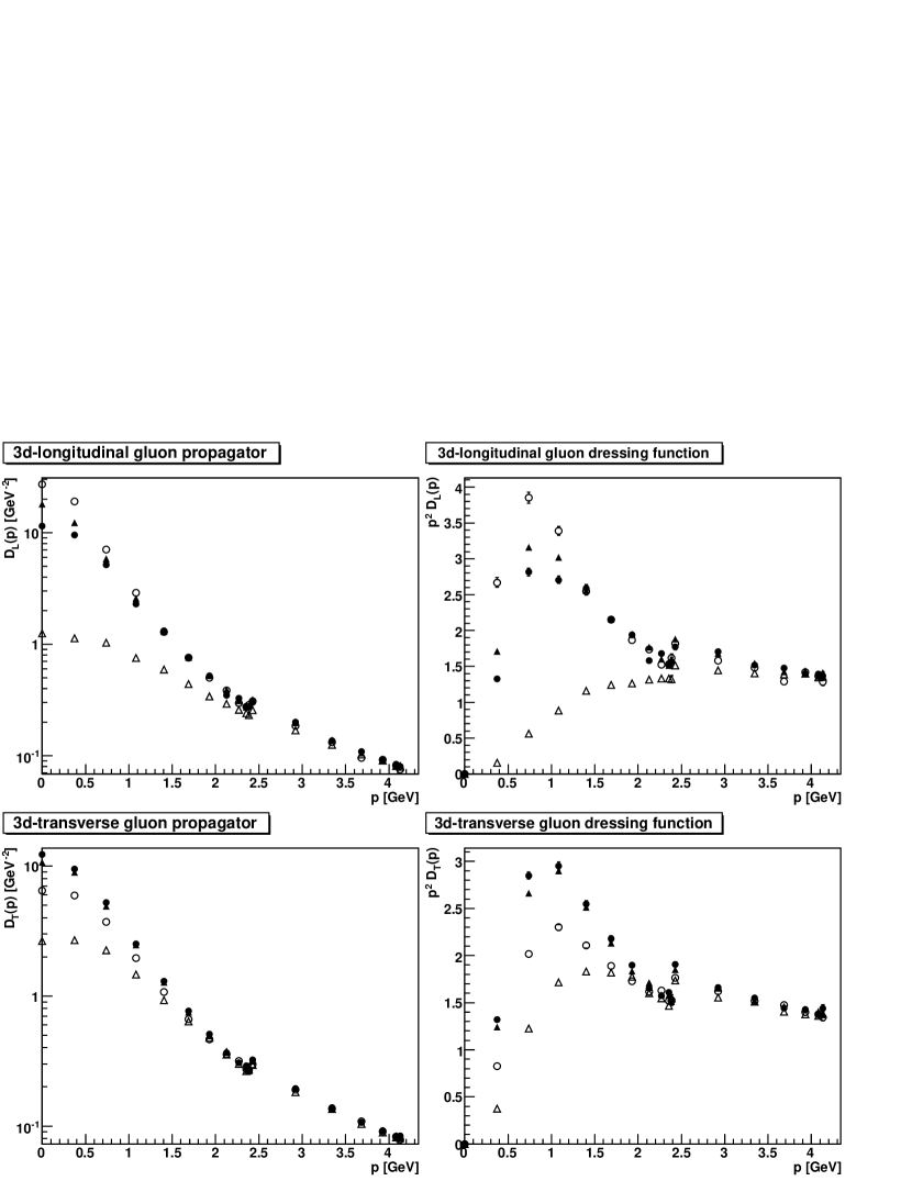
Figure 7: The 3d-longitudinal and 3d-transverse gluon propagators and dressing functions as a function of the temperature for the same spatial volume $V_{s}$ of approximately $(3.3$ fm$)^{3}$. We report data for the 3d-longitudinal propagator in the top-left panel and for the 3d-longitudinal dressing function in the top-right panel. Results for the 3d-transverse propagator are shown in the bottom-left panel and for the 3d-transverse dressing function in the bottom-right panel. Full circles, full triangles, open circles, and open triangles correspond to Setups 3 ($T=0$ MeV), 6 ($T\approx 119$ MeV), 8 ($T\approx 298$ MeV), and 13 ($T\approx 597$ MeV), respectively. Momenta respectively below and above 2.4 GeV are measured along the $x$-axis and along the spatial diagonal. The break at 2.4 GeV is due to violation of rotational invariance.

Figure 8: As figure 7, but considering for each temperature $T$ the largest spatial volume available. Full circles, full triangles, open circles, and open triangles correspond to Setups 3 ($T=0$ MeV), 7 ($T\approx 119$ MeV), 10 ($T\approx 298$ MeV) and 15 ($T\approx 597$ MeV), respectively.

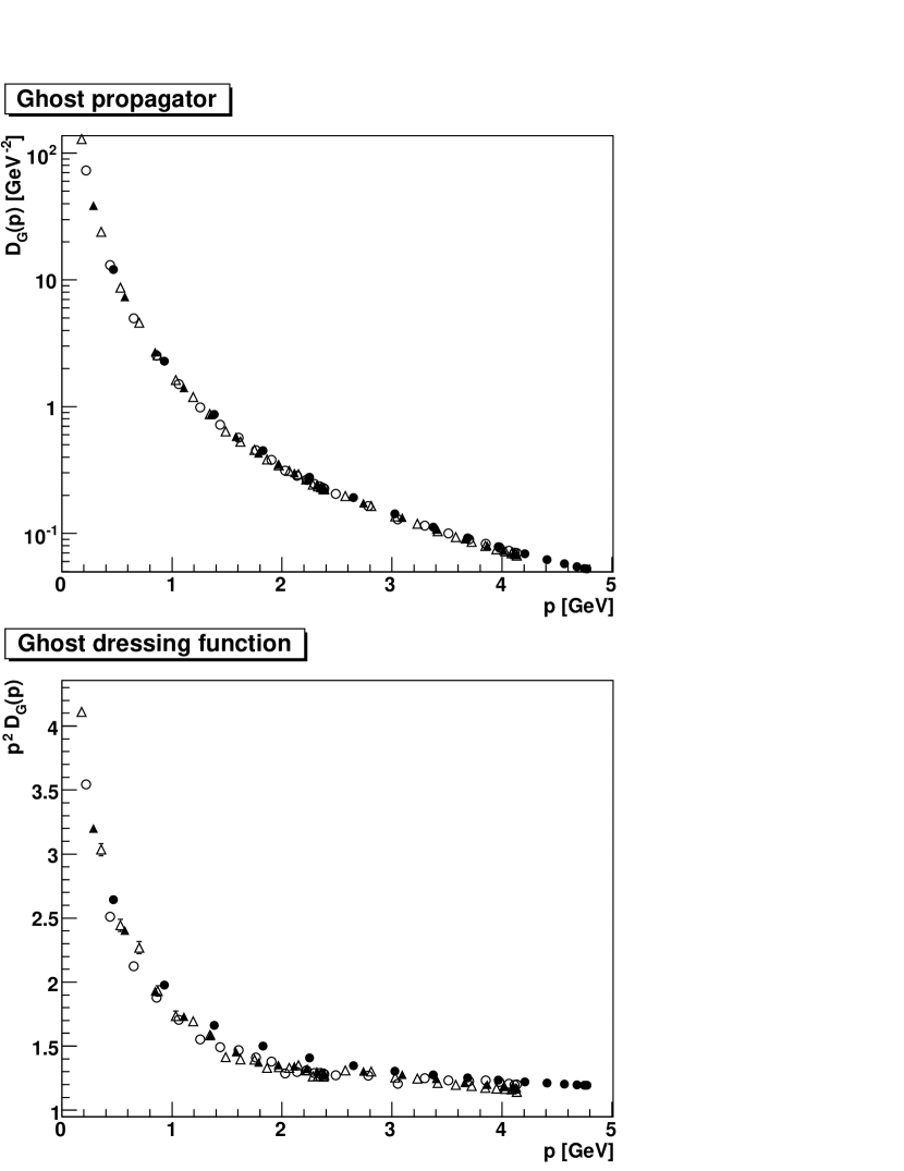
Figure 9: The ghost propagator and dressing function as a function of temperature. The top panel shows the ghost propagator and the bottom panel the corresponding dressing function. Full circles, full triangles, open circles, and open triangles correspond to Setups 4 ($T=0$ MeV), 7 ($T\approx 119$ MeV), 10 ($T\approx 298$ MeV) and 15 ($T\approx 597$ MeV), respectively.

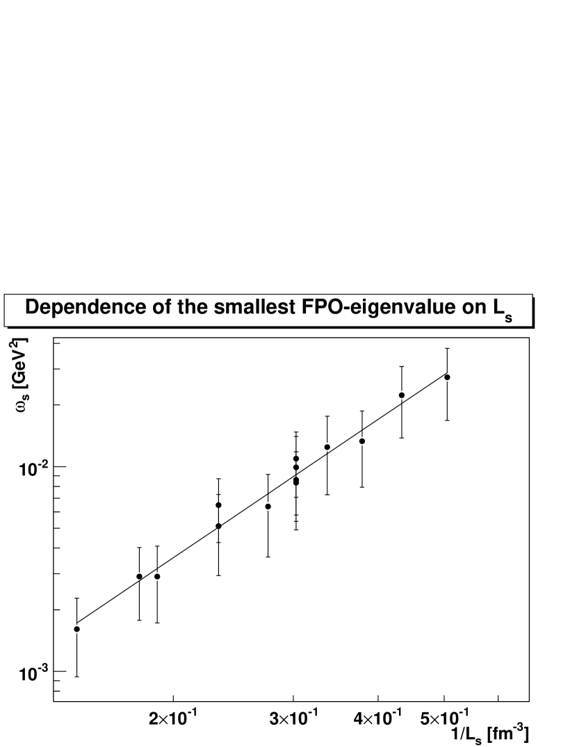
Figure 10: The dependence of the lowest eigenvalue $\omega_{s}$ of the FPO on the spatial extension $L_{s}$. The lines are fits of the type $cx^{-b}$. In the top figure, we show fits for each temperature separately. The fit parameters can be found in Table 2. Solid lines and circles are at $T=0$ MeV, dashed lines and squares are at $T\approx 119$ MeV, dotted lines and triangles are at $T\approx 298$ MeV while dashed-dotted lines and upside-down triangles are at $T\approx 597$ MeV. In addition to the Setups listed in Table 1 we obtained some of the data using lattice volumes 4$\times$18³ and $2\times 22^{3}$ at $\beta=2.3$. In the bottom figure we consider data for all the temperatures.

Here we present our calculations for gluon and ghost propagators in 4d at finite temperature. We consider four different temperatures, two of them below the thermodynamic transition (i.e. at zero temperature and at $T\approx 119$ MeV) and two above it (i.e. one at $T\approx 298$ MeV and the other at $T\approx 597$ MeV). Our runs are summarized in Table 1. Note that, for a time extension $N_{t}=4$, the critical coupling is $\beta=2.299$ Fingberg:1992ju , corresponding to $T_{c}\approx 295$ MeV. Here the calculations for this time extension have been done at $\beta=2.3$. Thus, the temperature $T\approx 298$ MeV is just above the thermodynamic transition, while the highest temperature ($T\approx 597$ MeV) corresponds to about twice the critical temperature $T_{c}$. This allows us to make contact with previous studies Cucchieri of the high-temperature phase, which investigated the gluon propagator for $T\gtrsim 2\,T_{c}$. In order to clarify possible finite-volume effects, we considered for each temperature three different spatial volumes. Due to memory limitations, the spatial sizes are chosen to depend on the temperature, the largest ones being at the highest temperatures, for which $N_{t}$ is smallest. We find that, in the ghost case, neither the propagator nor the dressing function show any visible volume or discretization effects within the statistical errors.

The volume dependence of the gluon propagators for the two Setups below the thermodynamic transition is shown in Fig.  4. As expected, at zero temperature, $D_{T}(p)$ and $D_{L}(p)$ coincide. In this case no clear volume dependence is observable, since the three spatial volumes are rather similar. At $T\approx 119$ MeV, $D_{T}(p)$ and $D_{L}(p)$ are already quite different (see discussion below for details). On the other hand, these two functions still do not show any strong volume dependence. Also note that the consequences of the violation of rotational symmetry are not stronger than in the zero-temperature case Cucchieri:2006tf ; Bloch:2003sk .

The situation is different when considering the high-temperature phase (see Fig.  5). Indeed, at $T\approx 298$ MeV, the two propagators show a clear, even though different, volume dependence. In particular, the 3d-longitudinal gluon propagator is enhanced at small momenta with increasing volume, while the 3d-transverse propagator becomes weaker in the IR with increasing volume. Finally, at $T\approx 597$ MeV, the volume dependence of the two propagators is similar, i.e. they both become smaller (in the IR region) as the volume increases. Moreover, the 3d-transverse propagator shows a distinct maximum at $p\approx 500$ MeV for the two largest volumes, while the 3d-longitudinal propagator seems to go to a constant at small $p$. These IR behaviors at $T\approx 2T_{c}$ are in agreement with previous studies Cucchieri . Note that the apparently stronger finite-size effects seen at $T\gtrsim T_{c}$ compared to the low-temperature cases are likely due to the larger spatial volumes (computationally) accessible in the high-temperature phase. Also note that a maximum in the 3d-transverse propagator in the high-temperature phase is observed already for a (spatial) lattice volume of $32^{3}$. At $T=0$, in the 4d case, one sees a clear maximum for $V\lesssim 32^{4}$ only when simulations are done in the strong-coupling regime Cucchieri:1997fy . Thus, finite-size effects for the transverse propagator seem to be smaller in the high-temperature phase, in agreement with previous results.

In Fig.  6 we check for discretization effects by comparing results for three different $\beta$ values for Setups that have, within a few percent, the same temperature (i.e. $T\approx 575$ MeV) and the same physical spatial volume $V_{s}\approx(3.35$ fm$)^{3}$. The two gluon propagators show a different behavior. Indeed, the 3d-transverse propagator is only weakly affected by the $\beta$ value at the smallest momenta, the effect being of the order of about 20 percent at most. On the other hand, for the 3d-longitudinal propagator, the effects in the IR are more pronounced, with variations of up to a factor of almost 2. This indicates that the scaling limit has not been reached yet for these Setups in the IR region. Thus, results for the 3d-longitudinal gluon propagator at momenta below 1.5 GeV should be taken with caution. Considering also the finite-volume effects discussed above, one probably needs to consider larger and finer lattices especially in the case of the 3d-longitudinal gluon propagator.

We can now compare the gluon propagators at different temperatures $T$. In particular, in Fig.  7 we consider Setups with the same physical spatial volume, while in Fig.  8 we show data using always the largest spatial volume available for a certain temperature. The results are similar in the two cases and in the the following we will mainly refer to Fig.  8. One clearly sees that at sufficiently large momenta the propagators at $T>0$ coincide with the ones at zero temperature. This is expected, since for $p\gg T$ zero-temperature perturbation theory should re-emerge. At smaller momenta, the 3d-transverse gluon propagator decreases monotonically as the temperature increases. Also, there is no sign of sensitivity to the thermodynamic transition. The situation is different for the 3d-longitudinal propagator. Indeed, in the IR region, it increases with $T$ when $T\lesssim T_{c}$, while it strongly decreases when going from $T\approx T_{c}$ to $T\approx 2\,T_{c}$. From these results it is tempting to assume that the 3d-longitudinal gluon propagator is largest at the thermodynamic transition. However, due to the strong finite-volume and discretization effects discussed above, a confirmation of this conjecture requires more systematic studies on larger and finer lattices. Note that, due to renormalization effects, all dressing functions should vanish logarithmically for sufficiently large momenta. Clearly this ultraviolet-asymptotic regime is not reached yet with our range of momenta.

Finally, from Fig. 9 we see that the Faddeev-Popov-ghost propagator does not show any visible temperature dependence for all temperatures $T$ considered here, in qualitative agreement with previous exploratory studies Langfeld:2002dd . We have also studied the spectrum of the Faddeev-Popov operator (FPO) ${\cal M}$ as a function of the temperature $T$. In particular, we checked if and at what rate the lowest eigenvalue $\omega_{s}$ of ${\cal M}$ vanishes in the infinite-volume limit Zwanziger . We recall that, in the 3d case, this eigenvalue vanishes faster than the lowest eigenvalue of the Laplacian Cucchieri:2006tf . The behavior of $\omega_{s}$ as a function of the spatial length $N_{s}a=L_{s}=(V_{s})^{1/3}$ is shown in Fig. 10. We fitted our data using a power-law function $cx^{-b}$. Results of these fits are reported in Table 2. We see that the exponent $b$ varies little with $T$ and is greater than or equal to $2$, i.e. the eigenvalue goes to zero at least as fast as the lowest eigenvalue of the Laplacian. The magnitude $c$ is also essentially unaffected by the temperature. This implies that, for the lattice volumes and the lattice spacings considered here, the eigenvalue $\omega_{s}$ (as a function of $1/L_{s}$) is already in the scaling region. By fitting all data we get an exponent $b=2.3(1)$ (see bottom of Fig. 10), to be compared with the exponent of approximately 2.6 in the 3d case Cucchieri:2006tf .

Summarizing our results for the propagators we find that 1) the ghost propagator does not have any noticeable temperature dependence, 2) the 3d-transverse propagator depends on the temperature, but it has the same (IR-suppressed) behavior below and above the thermodynamic transition and 3) the 3d-longitudinal gluon propagator does show a dependence on the temperature, with a different behavior above and below the phase transition and an apparent IR divergence at $T_{c}$. Moreover, at large $T$, the 3d-transverse propagator is suppressed in the IR limit, while the 3d-longitudinal one seems to behave as a massive particle, approaching a plateau for small $p$. Indeed, for all temperatures, volumes and discretizations, the 3d-longitudinal gluon dressing function vanishes in the IR. This implies that the 3d-longitudinal propagator is always less divergent than that of a massless particle. However, in order to check if the behavior is indeed that of a massive particle, one needs much larger physical volumes. Let us stress that the results obtained here at the highest temperature (i.e. $T\approx 2T_{c}$) agree qualitatively with those found in the dimensionally reduced theory Cucchieri:1999sz ; Cucchieri:2003di ; Cucchieri:2006tf and with previous studies of gluon propagators at high temperature Cucchieri .

A possible explanation of the above results will be discussed in Section V.

Table 2: Parameters for the fits in Fig. 10. Fits have been done with gnuplot.

$T$ [MeV]	$c$ [GeV2]	$b$
0	0.13(2)	2.3(2)
119	0.119(1)	2.00(1)
298	0.15(1)	2.31(6)
597	0.11(1)	2.19(5)

IV Dyson-Schwinger equations

Due to the strong finite-volume effects observed in the numerical data, it is important to complement the previous results with ones from the continuum and in the infinite volume, e.g. using DSEs. Let us recall that studies at finite $T$ using DSEs have already been presented in Maas:2005hs ; Gruter:2004bb . However, in both cases, in addition to the truncations usually employed at zero temperature vonSmekal , various approximations have also been performed in the solutions of the DSEs. Here, these additional approximations will be removed. In this section we discuss the (analytic) asymptotic IR solutions of the DSEs at any finite temperature, always assuming that external momenta $k$ obey $k\ll\Lambda_{\mathrm{QCD}}$. A (numerical) solution for all momenta, using the same truncation scheme as in Maas:2005hs ; Gruter:2004bb , is presented in Appendix D. Let us stress that the analysis presented here and in the Appendices B–D applies to any semi-simple gauge group without any qualitative change.

The setup for the system of DSEs at finite $T$ has already been extensively discussed elsewhere Maas:2005hs ; Gruter:2004bb ; Maas:2005rf . Let us recall that, in the far infrared, one can use the so-called ghost-loop-only truncation Maas:2005rf , which keeps only the leading infrared term arising in the derivation of the DSEs from the Faddeev-Popov-ghost term in the gauge-fixed Lagrangian. In the Gribov-Zwanziger scenario, this term dominates the action at low momenta.

Then, the equations for the zero (soft, $k_{0}=0$) modes are given by Maas:2005rf

$$\!\!\!\!\!\!\!\!\!\frac{1}{G(0,\vec{k})} = \tilde{Z}_{3}\,+\,\frac{g^{2}TC_{A}}{(2\pi)^{3}}\sum_{q_{0}}\int dq\,d\theta\,\left[A_{T}(0,q_{0},\vec{k},\vec{q})\,G(q_{0},\vec{q})\,Z(q_{0},\vec{q}-\vec{k})\,+\,A_{L}(0,q_{0},\vec{k},\vec{q})G(q_{0},\vec{q})H(q_{0},\vec{q}-\vec{k})\right]$$ (10)

$$\!\!\!\!\!\!\!\!\!\frac{1}{Z(0,\vec{k})} = Z_{3T}\,+\,\frac{g^{2}TC_{A}}{(2\pi)^{3}}\sum_{q_{0}}\int dq\,d\theta\,R(0,q_{0},\vec{k},\vec{q})\,G(q_{0},\vec{q})\,G(q_{0},\vec{q}+\vec{k})$$ (11)

$$\!\!\!\!\!\!\!\!\!\frac{1}{H(0,\vec{k})} = Z_{3L}\,+\,\frac{g^{2}TC_{A}}{(2\pi)^{3}}\sum_{q_{0}}\int dq\,d\theta\,P(0,q_{0},\vec{k},\vec{q})\,G(q_{0},\vec{q})\,G(q_{0},\vec{q}+\vec{k})\;.$$ (12)

Here, we use the definitions $G(k^{2})=k^{2}D_{G}(k^{2})$, $Z(k^{2})=k^{2}D_{T}(k^{2})$, $H(k^{2})=k^{2}D_{L}(k^{2})$, where $D_{G}(k^{2})$, $D_{T}(k^{2})$ and $D_{L}(k^{2})$ are, respectively, the ghost propagator and the transverse and longitudinal gluon propagators. The integral kernels $A_{T}$, $A_{L}$, $R$, $P$ and the angle $\theta$ are defined in Appendix B. Also, $T$ is the temperature, $g$ is the bare coupling constant and $C_{A}$ indicates the adjoint Casimir of the gauge group [for $SU(2)$, $C_{A}=2$]. The graphical representation of this system of equations is given in Fig. 11. Note that Eqs. (11–12) have been obtained from the tensor equation for the gluon propagator by contraction with generalizations of the projectors defined in Eqs. (2) and (3). These tensors are parameterized by the variables $\zeta$ and $\xi$ Maas:2005hs , which appear explicitly only in the integration kernels $R$ and $P$ (see Appendix B). Variations of these parameters can be used to investigate truncation artifacts and, in particular, the appearance of spurious divergences. Let us also note that the equations above reduce to the corresponding equations of a 3-dimensional Yang-Mills-Higgs system when the hard modes ($q_{0}\neq 0$) inside loops are neglected Maas:2004se . Then, due to the ghost-loop-only approximation, the Higgs field $H(0,\vec{k})$ decouples and $G(0,\vec{k})$ and $Z(0,\vec{k})$ become the dressing function of a pure 3d Yang-Mills theory Maas:2004se . In Appendix C we show that the solutions of Eqs. (10–12) at zero temperature coincide with the well-known solutions presented in Refs. vonSmekal . Finally, we remark that one can find different wave-function renormalization constants ($Z_{3T}$ and $Z_{3L}$) in the gluon equations due to possible finite contributions arising at non-zero temperature.

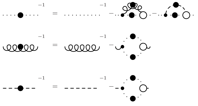
Figure 11: The DSEs in the ghost-loop-only approximation at finite temperature. Dotted lines represent ghosts, curly lines are used for the 3d-transverse gluons and dashed lines represent 3d-longitudinal gluons. Lines with a dot indicate a full propagator instead of a bare one. Vertices with a small dot are bare ones, while those with a large, empty dot represent full vertices. However, in our calculations these vertices are also taken to be bare.

Equations (10–12) can also be written as

$$\frac{1}{G(0,\vec{k})} = \tilde{Z}_{3}\,+\,\Pi_{G}(0,\vec{k})\,+\,\sum_{q_{0}\neq 0}\Pi_{G}(q_{0},\vec{k})$$ (13)

$$\frac{1}{Z(0,\vec{k})} = Z_{3T}\,+\,\Pi_{Z}(0,\vec{k})\,+\,\sum_{q_{0}\neq 0}\Pi_{Z}(q_{0},\vec{k})$$ (14)

$$\frac{1}{H(0,\vec{k})} = Z_{3L}\,+\,\sum_{q_{0}\neq 0}\Pi_{H}(q_{0},\vec{k})\;,$$ (15)

where we indicate with $\Pi_{i}$ the various self-energies. Note that, in the 3d-longitudinal equation the zero-component $q_{0}=0$ explicitly vanishes, since $P(0,0,\vec{k},\vec{q})=0$. This is a direct consequence of the tensor-structure of the ghost-gluon vertex. Thus, the behavior of the longitudinal mode $H(0,\vec{k})$ is entirely determined by the hard modes and depends only implicitly on the soft ones.

The treatment of the full system, given in Appendix D, justifies a-posteriori this ghost-loop-only truncation for momenta $k$ in the far IR limit. The same truncation is also sensible at zero temperature Fischer:2006vf . Furthermore, the ghost-gluon vertex is taken equal to the bare one. This approximation is supported by various calculations at zero Schleifenbaum:2004id ; Alkofer ; Ilgenfritz:2006gp ; Maas:2006qw and at infinite temperature Cucchieri:2006tf ; Schleifenbaum:2004id . Of course, when considering the far IR limit at non-zero temperature one needs to ensure the condition $|\vec{k}|\ll T$ for the external momenta. In this limit one obtains Maas:2005hs that the hard-mode dressing functions $Z(k_{0},\vec{k})$, $H(k_{0},\vec{k})$, $G(k_{0},\vec{k})$ become constant in the infrared, i.e. they have the behavior of the dressing function of massive particles. Thus, for $\vec{k}\to 0$, the dressing functions of the hard modes for the 3d-transverse gluon, the 3d-longitudinal gluon and the ghost, are respectively given by $A_{z}(k_{0})$, $A_{h}(k_{0})$ and $A_{g}(k_{0})$, which depend only on the Matsubara mode $k_{0}$. In order to find a solution to the system of equations (10–12), we need these IR constants to be bounded.

Finally, for the zero-modes ($k_{0}=0$) we consider the power-law ansätze

$$G(0,\vec{k}) = B_{g}\,k^{2\kappa}$$ (16)

$$Z(0,\vec{k}) = B_{z}\,k^{2t}$$ (17)

$$H(0,\vec{k}) = B_{h}\,k^{2l}\;,$$ (18)

which depends on the IR exponents $\kappa$, $t$ and $l$ and on the constant coefficients $B_{g}$, $B_{z}$ and $B_{h}$. Then, for all values of $\kappa$ and $t$, the self-energies $\Pi_{G}(0,\vec{k})$ and $\Pi_{Z}(0,\vec{k})$ take exactly the same form as in three dimensions Maas:2004se , i.e.

$$\Pi_{G}(0,\vec{k}) = -B_{g}\,B_{z}\,g^{2}TC_{A}\frac{2^{1-4\kappa}\Gamma(2+2\kappa)}{\kappa(3+4(-2+\kappa)\kappa)\Gamma\left(2\kappa+\frac{3}{2}\right)}y^{t+\kappa-\frac{1}{2}}$$ (19)

$$\Pi_{Z}(0,\vec{k}) = B_{g}^{2}\,g^{2}TC_{A}\frac{2^{-4(1+\kappa)}(-2+\zeta+2\kappa(\zeta-1))\Gamma(2+2\kappa)\sec(2\pi\kappa)\sin(\pi\kappa)^{2}}{\kappa^{2}(1+\kappa)\Gamma\left(2\kappa+\frac{3}{2}\right)}y^{2\kappa-\frac{1}{2}}\;,$$ (20)

where $y=k^{2}=\vec{k}^{2}$. Clearly, if these contributions are not exactly canceled (or dominated) by the remaining Matsubara sums, they will give the leading IR behavior of $G(0,\vec{k})$ and of $Z(0,\vec{k})$. In this case one finds a 3d-type behavior for all non-zero temperatures $T$. To show that this is indeed the case we observe that — by setting the hard-mode dressing functions equal to the constants $A_{g}(k_{0})$, $A_{z}(k_{0})$ and $A_{h}(k_{0})$ — the self-energies in the ghost equation (13) can be rewritten as

$$\Pi_{G}(q_{0}\neq 0,\vec{k})\,=\,g^{2}TC_{A}\left[-\left(\frac{A_{z}(q_{0})}{12\pi}\,+\,\frac{A_{h}(q_{0})}{96}\right)\frac{1}{|q_{0}|}+\left(\frac{A_{z}(q_{0})}{80\pi}\,+\,\frac{A_{h}(q_{0})}{1920}\right)\frac{\vec{k}^{2}}{|q_{0}|^{3}}+\vec{k}^{3}\pi(q_{0},\vec{k})\right]\;.$$ (21)

Here, the first term is logarithmically divergent and it can be absorbed in the renormalization constant. At the same time, the second term is sub-dominant when compared to the 3d-term, for values of $\kappa$ and $t$ permitted by integral convergence Maas:2004se , and is finite after summation over $q_{0}$. Finally, the function $\pi(\vec{k})$ vanishes identically as $\vec{k}\to 0$. Thus, the leading part of the ghost equation is the same as in the 3d-case, i.e. it is given by $\Pi_{G}(0,\vec{k})$, provided that the quantities $A_{z}(q_{0})$ and $A_{h}(q_{0})$ do not rise strongly as $q_{0}$ goes to infinity. Actually, due to asymptotic freedom, these quantities vanish logarithmically in the ultraviolet limit.

Finally, we should check that a 3d-type behavior is obtained for all non-zero temperatures $T$ also when considering the gluon equations (11) and (12). To this end, we first discard spurious divergences in these two equations. These are quadratic divergences, vanishing for $\zeta=3$ in the 3d-transverse equation (11) and similarly in the longitudinal equation (12). One can show that they are artifacts of the truncation scheme considered vonSmekal ; Maas:2005hs ; Maas:2005rf . After subtraction of these divergences, one can write the contributions of the hard-modes in the self-energies [see Eqs. (14–15)] as

$$\Pi_{Z}^{S}(q_{0},\vec{k})\;=\;\frac{\pi_{Z}(q_{0},\vec{k})}{k}\;,\qquad\qquad\Pi_{H}^{S}(q_{0},\vec{k})\;=\;\frac{\pi_{H}(q_{0},\vec{k})}{k}\;.$$ (22)

In both cases the function $\pi_{i}$ vanishes as $\vec{k}\to 0$, separately for each Matsubara term. Thus, the subtracted part cannot contribute to the IR behavior in the 3d-transverse equation. This is the case also after summing over $q_{0}$. On the other hand, the IR contributions from the un-subtracted self-energies cannot in general be neglected, as done when considering only the contributions (22). This requires, of course, a regularization vonSmekal of the spurious divergences. To achieve this, one can replace the approximately constant dressing functions of the hard modes by $A_{g}(q_{0})(q^{2}+q_{0}^{2})^{-\tau}$, which are clearly suppressed when $\tau>0$. This is the prescription commonly used for regularizing the divergences at zero temperature with $\tau=-\kappa$ Alkofer:2000wg ; Fischer:2006ub ; vonSmekal ; Zwanziger . Then, the integrals can be performed and in the limit $\vec{k}\to 0$ one finds

$$\Pi_{Z}^{D}(q_{0},\vec{k}\to 0) = -\frac{g^{2}TC_{A}}{k^{2}}\frac{(\zeta-3)\Gamma\left(\tau-\frac{1}{2}\right)}{32\pi^{3/2}\Gamma(2+2\tau)}(2\pi T)^{1-4\tau}\sum_{n\neq 0}A_{g}(n)^{2}|n|^{1-4\tau}$$ (23)

$$\Pi_{H}^{D}(q_{0},\vec{k}\to 0) = \frac{g^{2}TC_{A}}{k^{2}}\frac{\Gamma\left(2\tau+\frac{1}{2}\right)}{8\pi^{3/2}\Gamma(2+2\tau)}(2\pi T)^{1-4\tau}\sum_{n\neq 0}A_{g}(n)^{2}|n|^{1-4\tau}\;,$$ (24)

where $n=q_{0}/2\pi T$. These sums diverge for $\tau\leq 1/2$, due to the term $q_{0}^{1-4\tau}$. For $\tau=1/2$, this exponent becomes equal to $-1$, i.e. the sums are logarithmically divergent. Finally, for $\tau>1/2$, the sums are finite and they can (in principle) be resummed analytically. For example, for $A_{g}(n)=(2\pi T)^{2\tau}$ one finds that the sum in $n$ is equal to $2(2\pi T)^{4\tau}\zeta_{R}(4\tau-1)$, where $\zeta_{R}$ is the Riemann-$\zeta$ function. One should also note that the terms in (23–24) behave like $1/k^{2}$, i.e. like a mass term in the IR limit. In the 3d-transverse case — but not in the 3d-longitudinal case Maas:2005hs — this term may not be renormalized, as this is not allowed by gauge-invariance. If one does not allow either a divergence stronger than logarithmic (even though this cannot be excluded by the perturbative renormalization theorems) or different exponents $\tau$ to the 3d-transverse and to the 3d-longitudinal case, then the only possibility is to have $\tau>1/2$. For all such values of $\tau$, the contribution (23) is sub-leading in the 3d-transverse equation (14). At the same time, the screening mass in the 3d-longitudinal equation would then be solely due to the regularized contribution (24). This result is a consequence of the truncation scheme. In fact, due to the decoupling of the soft modes in the 3d-longitudinal equation [see Eq. (15)], the result is dominated by the hard modes, which are very sensitive to truncation artifacts, since they live on a scale that is effectively mid-momentum. Thus, the present truncation scheme is not able to yield a consistent description of the electric screening mass and a determination of its value is not possible. Nonetheless, the 3d-longitudinal gluon propagator seems to exhibit a screening mass, and thus gives likely a qualitatively correct description of the physics involved. This screening mass would not allow the 3d-longitudinal gluon propagator to modify the IR behavior of either the 3d-transverse gluon propagator or of the ghost propagator. Therefore, as shown above, these two propagators should behave at all non-zero temperatures exactly as in the three-dimensional case when one considers momenta much smaller than the temperature $T$ and than $\Lambda_{\mathrm{QCD}}$. It is then plausible that for momenta in the range $T\ll p\ll\Lambda_{\mathrm{QCD}}$ the gluon and the ghost propagator would still exhibit a behavior similar to that found in the four-dimensional case. This is also found in DSE studies in a finite volume fischer .

The behaviors described in this section are in agreement with calculations using renormalization-group techniques in a background-field gauge Braun:2006jd . Indeed, when going from $T=0$ to $T>0$, also in that case one finds a discontinuous change in the behavior of the running coupling, i.e. in the IR region the running coupling switches from a four-dimensional to an effectively three-dimensional behavior. Let us also note that previous studies using DSEs Gruter:2004bb had assumed that the zero-temperature behavior persists up to the thermodynamic transition. Here we have relaxed this hypothesis and eliminated some of the approximations of the numerical method employed in Gruter:2004bb , showing that the high-temperature results apply also to non-zero temperatures below the critical temperature $T_{c}$, a phenomenon previously interpreted as super-cooling Maas:2005hs .

V Summary

Let us summarize here the results obtained above for the 4d finite-temperature case. From our lattice calculations we have that:

• The 3d-transverse gluon propagator decreases as the temperature increases. It also seems to have smaller finite-volume effects (in the IR limit) and stronger IR suppression at high temperature than at zero temperature.

• The 3d-longitudinal gluon propagator at small momenta increases as the temperature goes from 0 to $T_{c}$, seems to diverge at $T_{c}$ and then drops as $T$ becomes larger, apparently reaching a plateau for small $p$. Also, in the IR limit, it is less divergent than the propagator of a massless particle, with a possible exception near the phase transition.

• The ghost propagator is nearly temperature-independent.

• The smallest eigenvalue of the Faddeev-Popov operator, considered as a function of the spatial lattice side $L_{s}$, goes to zero faster than $1/L_{s}^{2}$ as $L_{s}$ goes to infinity, for all temperatures.

From the DSEs we see that:

• The IR behavior of the gluon and ghost propagators changes abruptly from zero to any non-zero temperature.

• For momenta $p\ll(T,\Lambda_{\mathrm{QCD}})$, the ghost and the 3d-transverse gluon propagators show the same behavior obtained in the dimensionally reduced theory Maas:2004se ; Maas:2005hs and the IR behavior in the spatial sector is in accordance with the prediction of the Gribov-Zwanziger scenario Zwanziger ; Gribov .

• The 3d-longitudinal gluon is likely to have a dynamical mass at any non-zero temperature.

• These results can be connected continuously to perturbation theory at large $p$ (see Appendix D) and to the solution at zero temperature (see Appendix C).

As explained in Section IV above, the main assumption for these DSE results is that the electric screening mass is non-zero at all temperatures. Indeed, in the case of a null screening mass, one can find different solutions for the DSEs. In particular, the ghost propagator may or may not be IR divergent, while the 3d-transverse gluon propagator would still be IR suppressed Maas:2005rf . Note that the analytic asymptotic results from the DSE calculations are valid for momenta $p\ll\min(T,\Lambda_{\mathrm{QCD}})$. As already stressed in Section III.1, this range of momenta is not accessible with the lattice volumes used here. At intermediate momenta, DSE results agree qualitatively with the lattice results for all temperatures considered.

We can try to interpret these results by considering the Gribov-Zwanziger scenario applied to the 4d $T=0$ case and to the dimensionally reduced theory. As explained in Section III.1, this scenario is supported by lattice Cucchieri:2006xi ; Cucchieri:2003di ; Cucchieri:2006tf ; Cucchieri:1997dx ; Sternbeck:2005tk ; Silva and by DSE calculations vonSmekal ; Zwanziger ; Maas:2004se . Then, at $T>0$, due to the compactification of the time direction, the configuration space near the Gribov horizon should be essentially reduced to that of a three-(space-time)-dimensional system and, in the infinite-volume limit, the configurations should lie on the Gribov horizon Gribov for all temperatures and the Gribov-Zwanziger confinement scenario would apply to the so-called magnetic sector. As a consequence, one can remove the so-called IR problem Zahed:1999tg ; Maas:2005ym ; Linde:1980ts ; Blaizot:2001nr since an infrared suppressed 3d-transverse gluon propagator cancels the perturbative infrared divergences.

Based on the above considerations, our results may be organized into the following scenario:

• At non-zero temperature, the time-like momenta are no longer continuous, but discrete. Due to this gap, the properties of configurations near the Gribov-horizon are changed. This modifies (probably only quantitatively) the spectrum of the Faddeev-Popov operator. Thus, the enhancement for small eigenvalues observed at $T=0$ Sternbeck:2005vs should still be present and the IR enhancement of the ghost propagator might be reduced but not eliminated. This is verified by our lattice data.

• The consequences for the 3d-transverse gluon and the 3d-longitudinal gluon are different, due to the vector character of the ghost-gluon interaction. In particular, in the 3d-transverse case, the coupling is not modified in the DSEs and this propagator is still IR suppressed. Moreover, this suppression is actually stronger due to the structure of the 3d-transverse gluon-ghost interaction. This is also suggested from our lattice data.

• On the other hand, the coupling of the ghost to the 3d-longitudinal gluon becomes gapped. Thus, the solution of the DSEs is consistent with these gluons acquiring a real (dynamical) mass, being no longer IR suppressed. This 3d-longitudinal screening mass is generated solely by the hard modes, leading likely to a mass of the order of the temperature, which is the characteristic scale of the hard-modes. In addition, this is observed in lattice calculations at very high temperatures Cucchieri . At the same time, this screening mass should, similarly to the hard modes, be sensitive to the phase transition. This is partially seen from our lattice data, since the longitudinal propagator is sensitive to the phase transition and seems to reach a plateau at small $p$ for $T>T_{c}$.

• Finally, it should be noted that the presence of an electric screening mass does not imply that the 3d-longitudinal gluon is deconfined or an observable particle. Indeed, a massive particle does not necessarily have a positive-definite spectral function Maas:2004se ; Maas:2005hs ; Maas:2005rf . Moreover, the $A_{0}$-field is (at the perturbative level) member of a BRST-quartet at any finite temperature Das:1997gg . These considerations would imply that no gluon is part of the physical spectrum also at any $T>0$.

A number of predictions follows from the scenario presented above, which could in principle be further tested using lattice calculations at sufficiently large volumes and with sufficiently fine discretization. The main predictions are:

• For all temperatures, the 3d-transverse gluon propagator is IR suppressed, while the ghost propagator is IR enhanced.

• When $p\ll(T,\Lambda_{\mathrm{QCD}})$ the IR behavior of the 3d-transverse gluon propagator and of the ghost propagator is quantitatively different from the behavior observed for $T\ll p\ll\Lambda_{\mathrm{QCD}}$, the latter one being similar to the behaviors observed at zero temperature with momenta $p\ll\Lambda_{\mathrm{QCD}}$.

• The 3d-longitudinal gluon propagator is null at zero momentum only at $T=0$, while it goes to a finite (non-zero) value at $p=0$ for all temperatures $T>0$. This propagator is sensitive to the phase transition.

Of course, it would be interesting to compare our numerical results to a similar study for the $SU(3)$ group, for which a different kind of thermodynamic transition is expected Karsch:2001cy . Note that first investigations, with and without dynamical quarks, have been performed in Furui:2006py .

VI Conclusions

We have presented an analysis of gluon and ghost propagators at finite temperature, using lattice gauge theory and DSEs. Results using these two approaches seem to be (at least at the qualitative level) consistent with each other. In particular, when the temperature is turned on, one finds different effects for 1) the temporal sector, which includes the soft 3d-longitudinal gluon, 2) the spatial sector, containing the soft ghost and the soft 3d-transverse gluon and 3) the hard sector with the (essentially perturbative) hard modes. In the spatial sub-sector, the IR behavior is similar to that of a 3-dimensional theory and the correlation functions agree with those expected from the Gribov-Zwanziger confinement scenario. Also, their dependence on the temperature is smooth. On the contrary, the temporal sector is sensitive to the thermodynamic transition, being screened and decoupling at the scale of the temperature. Nevertheless, our results are consistent with the possibility that all gluons are confined at all temperatures. Note that this does not alter the bulk thermodynamic properties, which still have a Stefan-Boltzmann-like behavior Maas:2004se ; Maas:2005hs ; Zwanziger:2006sc ; Zwanziger:2004np . These results can be understood by considering the Gribov-Zwanziger confinement scenario at $T\neq 0$. As a consequence, gluon confinement is not affected by the thermodynamic transition. This would explain the presence of non-perturbative effects in the high-temperature phase and the confining properties of the dimensionally-reduced theory in the infinite-temperature limit.

One should, however, recall that these results are affected by various (technical) limitations. Indeed, much larger and finer lattices and more sophisticated DSE schemes are needed in order to obtain a complete understanding of the effect of the temperature in the gluonic sector of Yang-Mills theory.

Finally, let us note that the introduction of dynamical quarks should not modify the Gribov-Zwanziger scenario and, as a consequence, the scenario described above. At the same time, the chiral transition should also not be affected by the IR arguments considered here, as the relevant dynamics occurs at the scale of $\Lambda_{\mathrm{QCD}}$ (see e.g. Fischer:2006ub ).

Appendix A Asymmetric lattices

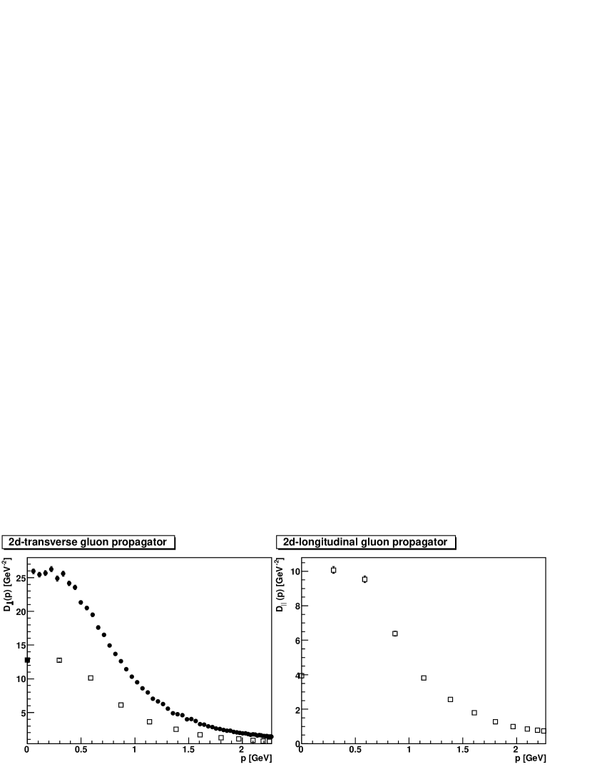
Figure 12: The orthogonal $D_{\perp}(p)$ and the parallel $D_{\parallel}(p)$ components of the gluon propagator evaluated using the (three-dimensional) strongly-asymmetric lattice $24^{2}\times 128$ at $\beta=4.2$. Open symbols correspond to momenta ($p_{s}$) along one of the short sides of the lattice, while full symbols correspond to momenta ($p_{l}$) along the long side of the lattice. Here we considered 420 configurations and the same settings used for Setup 15. Note that, due to the Landau gauge condition, one has $D_{\parallel}(p_{l},0)=0$ for all momenta $p_{l}$.

When using asymmetric lattices at $T=0$ (e.g. if the time extension of the lattice is larger than the spatial ones) it is convenient to consider the two scalar gluon propagators given by $D_{\perp}(p)=D_{ii}(p)/(d-1)$ and $D_{\parallel}(p)=D_{00}(p)$, where in the first case we sum over the spatial indices $i$ only. In Fig. 12 we report the results obtained for these two different tensor components of the gluon propagator when considering an asymmetric lattice of size $24^{2}\times 128$ (at $\beta=4.2$). Let us note that the total volume in this case is roughly the same as for a $40^{3}$ lattice. In this symmetric case, one clearly sees a maximum in the propagator for a momentum $p\approx 400$ MeV (see Section III.1 and the top plot in Fig. 1). In the asymmetric case, on the contrary, it is evident that the two tensor components show a very different behavior and that the behavior of the orthogonal propagator $D_{\perp}(p)$ depends on the type of momentum considered, i.e. along the short axis of the lattice ($p_{s}$) or along the long axis of the lattice ($p_{l}$). Also, there is no clear evidence of a maximum, even when considering $D_{\perp}(p_{l})$. Moreover, as observed already in Cucchieri:2006za , the IR suppression obtained using an asymmetric lattice $N_{s}^{d-1}N_{t}$ with $N_{t}\gg N_{s}$ is usually smaller than the suppression found on a symmetric lattice with volume $N_{t}^{d}$. This effect clearly reduces the advantages of using asymmetric lattices.

When considering asymmetric lattices, one might also use asymmetric couplings in order to have the same physical extent in all directions. This would probably reduce the systematic effects observed in Cucchieri:2006za , while keeping the numerical costs of the simulations small.

Appendix B Integral kernels

Here we define the integral kernels obtained with the ghost-loop-only truncation [see Eqs. (10)–(12)]. We use the following notation

$$\left.\begin{array}[]{l}y=k^{2}=k_{0}^{2}+\vec{k}^{2}\,;\quad\quad x=q^{2}=q_{0}^{2}+\vec{q}^{2}\,;\quad\quad k=|\vec{k}|\,;\quad\quad q=|\vec{q}|\\[5.69054pt] u=x+y+2k_{0}q_{0}-2\vec{k}\cdot\vec{q}\,;\quad\quad v=(\vec{k}-\vec{q})^{2}\\[5.69054pt] z=x+y+2k_{0}q_{0}+2\vec{k}\cdot\vec{q}\,;\quad\quad w=(\vec{k}+\vec{q})^{2}\\[2.84526pt] \theta=\arccos{\left(\vec{k}\cdot\vec{q}/kq\right)}\;.\end{array}\right.$$ (25)

Then, the kernels in the ghost self-energy (10) are given by

$$A_{T}(k_{0},q_{0},\vec{k},\vec{q}) = \frac{q^{2}(\vec{k}\cdot\vec{q}-k^{2}q^{2})\sin\theta}{xyuv}\,,$$ (26)

$$A_{L}(k_{0},q_{0},\vec{k},\vec{q}) = -\frac{q^{2}\left[k_{0}q^{2}+k^{2}q_{0}-(k_{0}+q_{0})\vec{k}\cdot\vec{q}\right]^{2}\sin\theta}{xyvu^{2}}\;.$$ (27)

At the same time, in the 3d-transverse gluon equation (11), the kernel is equal to

$$R(k_{0},q_{0},\vec{k},\vec{q})\,=\,-\frac{q^{3}\left[-q+k(\zeta-1)\cos\theta+q\zeta\cos\theta^{2}\right]\sin\theta}{2xyz}\,,$$ (28)

while in the 3d-longitudinal equation (12) it is

$$P(k_{0},q_{0},\vec{k},\vec{q}) = \frac{1}{y^{2}xz}[q^{2}(q_{0}\{-2k_{0}^{2}(k_{0}+q0)(\xi-1)+k^{2}[k_{0}-\xi(k_{0}-q_{0})]\}$$ (29)

$$\qquad\quad-kqk_{0}\{k_{0}(\xi-1)+2q_{0}(2\xi-1)\}\cos\theta+k_{0}^{2}q^{2}\xi\cos\theta^{2})]\sin\theta\;.$$

Note that the 3d-transverse equation (11) has been contracted with a tensor parameterized by a variable $\zeta$ Maas:2005hs . This variable appears only inside the integration kernel (28). The case $\zeta=1$ corresponds to the projector given in Eq. (2). The same has also been done for the 3d-longitudinal equation (12), with the variable $\xi$. Again, it only appears inside the integration kernel (29). For the zero mode ($k_{0}=0$), $\xi$ factorizes in all terms and can thus be eliminated from the equation. Hence the equation depends only implicitly on $\xi$, due to the hard modes Maas:2005hs .

Appendix C Vacuum solution

As said in Section IV above, a necessary requirement is that Eqs. (10–12) reproduce the well-known vacuum behavior vonSmekal at $T=0$. To show this, it is useful to consider linear combinations of Eqs. (11) and (12). In particular, we consider a combination with weights given by $2/3$ and $1/3$. We also introduce a second combination with weights equal to $1$ and $(\zeta-3)/2$. At $T=0$ the Matsubara sums become integrals. After performing these integrals in the equations obtained by considering both linear combinations, we find

$$f(k) = \frac{2}{3Z}+\frac{1}{3H}=-g^{2}B_{g}^{2}\frac{4^{-3-2\kappa}\pi^{2}(1+\kappa)(3+2\kappa)(-6-4\kappa+\zeta(3+4\kappa))\csc(2\pi\kappa)}{3\Gamma(1-\kappa)^{2}\Gamma\left(\kappa+\frac{5}{2}\right)^{2}}y^{2\kappa}$$ (30)

$$l(k) = \frac{1}{Z}+\frac{\zeta-3}{2}\frac{1}{H}=Z_{3T}+\frac{\zeta-3}{2}Z_{3L}+\frac{\rho(k)}{k^{2}}\;,$$ (31)

with $y=k^{2}$. The function $\rho(k)$ vanishes for $k\to 0$. Hence, for $\kappa\geq 0.5$, $l(k)$ is sub-leading compared to $f(k)$. This yields

$$Z(k) = \frac{2(\zeta-4)}{3(\zeta-3)f(k)-2l(k)}$$ (32)

$$H(k) = \frac{4-\zeta}{3f(k)-2l(k)}\;.$$ (33)

Without considering the trivial case $\zeta=4$ and neglecting the sub-leading quantity $l(k)$, these two functions coincide only in the case $\zeta=1$. For other values of $\zeta$ the dressing functions $Z(k)$ and $H(k)$ will have the same leading IR behavior, but they will differ by a constant factor. This is simply an artifact of the non-$O(4)$-invariant projection considered. Thus, for the remaining discussion we can set $\zeta$ equal to 1.

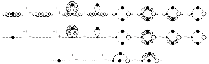
Figure 13: The truncated Dyson-Schwinger equations at finite temperature. The wiggly lines represent transverse gluons, the dashed lines longitudinal gluons and the dotted lines denote ghosts. Lines with a full dot represent self-consistent propagators while small dots indicate bare vertices. The open-circled vertices are full and must be constructed in a given truncation scheme. A bare ghost-gluon vertex and modified bare gluon vertices have been used here.

By using the above results and the IR ansatz (16), the ghost equation gives the relation

$$y^{-\kappa}=-g^{2}B_{g}^{2}B_{z}\frac{3\pi\Gamma(-2\kappa)\Gamma(2+\kappa)\csc(\pi\kappa)}{\kappa^{2}(2-3\kappa+\kappa^{2})\Gamma(-\kappa)^{3}\Gamma(2+2\kappa)}y^{\kappa+t}\;.$$ (34)

Here and henceforth the sub-leading terms proportional to $\rho(k)$ have been dropped. Clearly, this relation can be satisfied for all values of $y$ (in the infrared limit) only if the four-dimensional relation vonSmekal ; Watson:2001yv

$$2\kappa+t=0\;$$ (35)

is satisfied. By dividing equations (30) and (34), inserting the power-law ansätze (16–18) and setting $Z=H$, one finds a consistency condition for $\kappa$, i.e.

$$1=\frac{(2-\kappa)(\kappa-1)}{12(3+4\kappa(2+\kappa))}\;,$$ (36)

This equation is identical to the $T=0$ equation and is solved by $\kappa\approx-0.595353$ Zwanziger ; Lerche:2002ep .

Appendix D The full system

In this section we consider the system of DSEs truncated at the one-loop level (see Fig. 13). This truncation has already been discussed in detail in Refs. Maas:2005hs ; Maas:2005rf for the finite (i.e. nonzero) temperature case.

D.1 Perturbation theory and truncation artifacts

Many direct experimental verifications of QCD are performed in a regime where perturbation theory is applicable. Thus, any non-perturbative treatment must make contact with it. In the case of DSEs (at the presented truncation level) this implies recovering the resummed leading order perturbation theory Alkofer:2000wg ; Fischer:2006ub ; vonSmekal . Of course, at finite temperature $T$, the vacuum perturbation theory is expected to be recovered only at momenta large compared to $T$.

In order to show that this is the case, the first step is to identify and remove the spurious quadratic divergences Alkofer:2000wg ; Fischer:2006ub ; vonSmekal . Since the summation over the Matsubara frequencies extends to infinity, spurious divergences might depend on the order of integration and summation. Furthermore, it is possible that a contribution is finite with respect to integration but not to summation and vice-versa. Of course, only the region corresponding to large $n$ is relevant for the analysis of spurious divergences. In this limit, the difference between two consecutive Matsubara frequencies becomes negligible and the summation becomes equivalent to an integration. One can then replace $|\vec{q}|$ by $q\sin\eta$ and $q_{0}$ by $q\cos\eta$ (with $q^{2}=q_{0}^{2}+\vec{q}^{2}$) in the integral kernels $K(q)$ appearing in DSEs. Since the angular integration over $\eta$ yields no divergences, it is sufficient to replace all integral kernels $K(q)$ by the prescription

$$K(q)\to K(q)-\frac{1}{q^{2}}\lim_{q\to\infty}q^{2}K(q)\;.$$ (37)

The resulting integrals have no spurious quadratic divergences, but only the usual logarithmic one. One could absorb the subtracted part in gauge non-invariant counter-terms, as they originate purely from violation of gauge invariance. On the other hand, as discussed in Section IV above, this affects the IR behavior of the solutions. To surpass this problem constructively, the electric screening mass is here explicitly renormalized to a fixed value $m_{r}=g^{2}T$, since this is allowed by gauge invariance Maas:2005hs . Note that this prescription is sub-leading in the ultraviolet and does not affect perturbation theory. At the same time, the corresponding terms in the 3d-transverse equation can be dropped, as they are sub-leading both in the IR and in the ultraviolet limit. The only exception is the soft-mode contribution, which is treated as in the infinite-temperature limit Maas:2004se . As for the genuine tadpoles, they could in principle give a finite contribution. However, when removing the quadratic divergences according to (37), they vanish identically. Thus, also at finite temperature, the tadpoles contribute only a pure divergence, which can be absorbed in gauge non-invariant counter-terms. Also note that this implies that all spurious divergences are not affected by a finite temperature. This is to some extent not surprising, as the usual divergences in quantum field theory may not be affected by a finite temperature Das:1997gg .

As a second step, we have now to fix the renormalization prescription for the (physical) logarithmic divergences. In order to recover the 3d-theory in the infinite-temperature limit, two aspects have to be considered in the renormalization prescription Maas:2005hs . Firstly, one needs a finite 3d-coupling. To this end, one requires the quantity $g^{2}T$ to be fixed to $\Lambda_{\mbox{\footnotesize QCD}}$ for large temperatures Maas:2005hs ; Maas:2005rf . This implicitly defines a temperature-dependent renormalization scheme and automatically fixes the renormalization scale $\mu$ as a function of $T$ by the running of the coupling constant $g^{2}/(4\pi)=\alpha_{S}$. At the same time, a smooth zero-temperature limit is obtained using the prescription

$$\mu=\Lambda_{\mbox{\footnotesize QCD}}\left\{\exp\left[\frac{\left(\sqrt{8}\pi\right)^{2}}{\beta_{0}}\right]-1+\exp\left(\frac{8\pi^{2}T}{\beta_{0}\Lambda_{\mbox{\footnotesize QCD}}}\right)\right\}\;.$$ (38)

Here $\beta_{0}$ is the first coefficient of the $\beta$-function. Then, according to the perturbatively resummed 1-loop result, the largest value attained by $\alpha_{S}$ is $1$, i.e. $g^{2}=4\pi$.

Secondly, the wave function must be renormalized such that the dressing functions become unity at infinite momentum for $T\to\infty$. This is guaranteed by selecting the subtraction point

$$s=10^{4}\Lambda_{\mbox{\footnotesize QCD}}+2\pi T\;.$$ (39)

Note that the term $10^{4}\Lambda_{\mbox{\footnotesize QCD}}$ has been added to renormalize perturbatively at zero temperature. Clearly, the choice of temperature-dependent values for $s$ and $\mu$ entails that the renormalization constants will also contain finite temperature-dependent contributions.

The regularization and renormalization are performed as in Refs. Maas:2005hs ; Maas:2005rf by adding explicit counter-terms. This makes multiplicative renormalizability manifest. The renormalization conditions are

$$G(s)=Z(s)=H(s)=1\;.$$ (40)

They implement the requirement

$$G^{2}(s)Z(s)=G^{2}(s)H(s)=1$$ (41)

from Slavnov-Taylor identities (STI) at zero temperature vonSmekal . Note that this prescription does not allow any freedom in the values of the IR pre-factors in the ansätze (16–18). This renormalization scheme is explicitly independent of any Matsubara frequencies, and thus it suffices to determine the wave function renormalization constants in the soft equations. On the other hand, this renormalization scheme only works if performed at momenta sufficiently far in the perturbative regime, since $g$ has only been included to the leading perturbative order.

In order to recover perturbation theory, the ultraviolet asymptotic dressing functions must be given by the renormalization-group-improved perturbative propagators Yndurain:1999ui

$$G(p) = G(s)\left[\omega\log\left(\frac{p^{2}}{s^{2}}\right)+1\right]^{\delta}$$ (42)

$$Z(p)=H(p) = Z(s)\left[\omega\log\left(\frac{p^{2}}{s^{2}}\right)+1\right]^{\gamma}$$ (43)

$$\omega = -\frac{3g^{2}(\mu)C_{A}}{64\pi^{2}\delta}$$ (44)

$$\delta = -\frac{1}{2}(\gamma+1)=-\frac{9}{44}\;.$$ (45)

This also implies that the longitudinal and transverse gluon propagators must coincide at sufficiently large momenta $p$. At the same time, any kind of gauge-invariance violation must vanish, i.e. the propagators should become independent of the variables $\zeta$ and $\xi$.

It thus remains to test whether the truncation scheme permits this. At $T=0$ it has been found that only a dressed three-gluon vertex yields the correct perturbative solution vonSmekal . Thus, we consider the Bose-symmetric ansatz

$$\Gamma(p,q,k)_{\mu\nu\rho} = A(q,p,k)\,\Gamma(p,q,k)^{(\mathrm{tl})}_{\mu\nu\rho}(p,q,k)$$ (46)

$$= a\;G\left(\frac{1}{2}\left(q^{2}+p^{2}+k^{2}\right)\right)^{a_{G}}Z\left(\frac{1}{2}\left(q^{2}+p^{2}+k^{2}\right)\right)^{a_{Z}}\Gamma(p,q,k)^{(\mathrm{tl})}_{\mu\nu\rho}(p,q,k)\;.$$ (47)

Here, $\Gamma$ and $\Gamma^{(\mathrm{tl})}$ are respectively the full and the tree-level vertex and the constants $a$, $a_{G}$ and $a_{Z}$ will be chosen such that the propagators (42–43) are a solution of the system. Of course the above ansatz is valid only at high momenta. The low-momentum case, for which $Z\neq H$, will be discussed below.

Finally, it is sufficient to inspect the limit $p\gg p_{0}$ in a given equation, which thus reduces to the corresponding soft equation. As only the large-momentum behavior is relevant, the integrals can be treated with a lower cutoff $p$. Furthermore, the denominators can then be expanded in inverse powers of the integration momentum up to ${\cal O}(q^{-3})$. Approximating further internal dressing functions by $G(p+q)\approx G(q)$ etc. vonSmekal , a simple set of equations is obtained

$$\frac{1}{G(p^{2})} = \tilde{Z}_{3}-\frac{3g^{2}C_{A}}{64\pi^{2}}\int_{p^{2}}^{\Omega^{2}}dy\frac{G(y)Z(y)}{y}$$ (48)

$$\frac{1}{Z(p^{2})} = Z_{3T}+\frac{g^{2}C_{A}(3\zeta-5)}{384\pi^{2}}\int_{p^{2}}^{\Omega^{2}}dy\frac{G(y)^{2}}{y}-\frac{g^{2}C_{A}(47+3\zeta)}{384\pi^{2}}\int_{p^{2}}^{\Omega^{2}}dy\frac{A(y,y,p^{2})Z(y)^{2}}{y}$$ (49)

$$\frac{\xi}{Z(p^{2})} = \xi Z_{3L}-\frac{g^{2}C_{A}\xi}{192\pi^{2}}\int_{p^{2}}^{\Omega^{2}}dy\frac{G(y)^{2}}{y}-\frac{25g^{2}C_{A}\xi}{192\pi^{2}}\int_{p^{2}}^{\Omega^{2}}dy\frac{A(y,y,p^{2})Z(y)^{2}}{y}\;.$$ (50)

(The integral kernels and other details of these equations can be found in Maas:2005rf .) In these equations, the asymptotic form (43) has already been used to replace $H$ by $Z$ and $y=q^{2}=q_{0}^{2}+\vec{q}^{2}$. Note that the third equation is the original 3d-longitudinal equation and the $\xi$-dependence can obviously be removed. The wave function renormalization constants are chosen to cancel exactly the upper boundary of the integrals, thus rendering the equations finite and independent of the regulator $\Omega$.

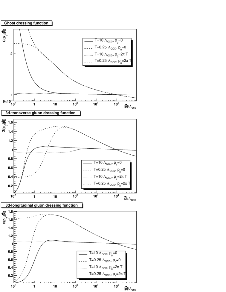
Figure 14: Numerical results from the Dyson-Schwinger equations at two temperatures in units of $\Lambda_{\mbox{\footnotesize QCD}}$ for the soft mode $p_{0}=0$ and for the first hard mode $p_{0}=2\pi T$ (4 and 5 modes have been calculated explicitly in the high and in the low temperature case, respectively). We show in the top, middle and bottom panel the dressing functions of the ghost, of the 3d-transverse gluon and of the 3d-longitudinal gluon, respectively. The different ultraviolet behavior for different temperatures is due to the temperature-dependent choice of the renormalization conditions.

One can then check that the ghost equation (48) is solved by (42–43). This yields the relation (45) between $\gamma$ and $\delta$ and the value of $\omega$ [see Eq. (44)]. On the other hand, the value of $\delta$ is not fixed. The remaining task is the choice for $A(y,y,p^{2})$. Using the ansatz (47) in the 3d-transverse equation (49), one finds for the parameters $a_{Z}$ and $a$ the conditions

$$a_{Z} = \frac{-2-6\delta+a_{G}\delta}{1+2\delta}$$ (51)

$$a = \frac{-18-41\delta+3\delta\zeta}{\delta(47+3\zeta)}\;.$$ (52)

At the same time, the equation becomes independent of $a_{G}$. In the 3d-longitudinal equation (50) one finds again for $a_{Z}$ the solution (51). On the other hand, $a$ is determined to be given by

$$a=\frac{-9-19\delta}{25\delta}\;.$$ (53)

Incidentally, there is only one value of $\delta$ that at the same time removes the $\zeta$-dependence in the 3d-transverse equation and yields the same $a$ value in both the 3d-transverse equation and in the 3d-longitudinal equation. This value is $\delta=-9/44$, which coincides with the result from the renormalization-group-improved perturbation theory (45). For this value, one finds $a=1$ in both equations above. Thus, the condition of gauge invariance uniquely requires for this truncation scheme the correct value of $\delta$. This is quite convenient, although likely accidental.

Let us note that it is always possible to rewrite $a=Z_{1}b$ with an arbitrary value for $Z_{1}$, thus realizing the STI $Z_{1}=Z_{3}/\tilde{Z}_{3}$ deliberately by fixing $b$ appropriately.

Finally, as said above, we can consider the low-momentum form of the three-gluon vertex. To this end, we replace $G^{a_{G}}Z^{a_{Z}}$ in Eq. (47) with the quantity $G^{na_{GT}/3+ma_{GL}/3}Z^{na_{Z}/3}H^{ma_{H}/3}$. Here, $n$ and $m$ are the number of 3d-transverse and 3d-longitudinal legs. The exponents $a_{Z}$ and $a_{H}$ are chosen to satisfy (51) for $a_{G}=a_{GT}$ and $a_{G}=a_{GL}$, respectively. A convenient choice for the remaining parameters $a_{GT}$ and $a_{GL}$ is

$$a_{GT} = \frac{2t(1+3\delta)}{t\delta+\kappa+2\delta\kappa}$$ (54)

$$a_{GL} = \frac{2l(1+3\delta)}{l\delta+\kappa+2\delta\kappa}\;,$$ (55)

where $\kappa$, $t$, and $l$ are the IR exponents of the dressing functions (16–18). This yields an IR (positive) constant three-gluon vertex. Although this is not in agreement with recent results on the IR behavior of this vertex Alkofer ; Maas:2006qw ; vrtx4d , this is irrelevant, because the gluon loops are still IR sub-leading.

It remains to select for the numerical solution at intermediate momenta the Matsubara frequency for which the dressing functions should be evaluated in the function $A$. The quantity $\sqrt{q_{0}^{2}+p_{0}^{2}+(q_{0}+p_{0})^{2}}/(4\pi T)$ is, apart from $p_{0}=q_{0}=0$ (the most relevant case), in general not an integer. As there is no obvious possibility, the largest integer smaller than this expression will be taken as the Matsubara frequency at which the expression is evaluated.

Note that in the present approach the use of the Matsubara formalism and of the vacuum perturbation theory in an asymptotically-free theory does not contradict the Narnhofer-Thirring theorem Narnhofer:1983hp . In fact, solving the set of DSEs self-consistently is not equivalent to expanding around a free system and the obtained propagators thus describe thermal quasi-particles.

D.2 Numerical solution

A full numerical solution of the DSEs (for an explicit form of the equations see Maas:2005hs ) and the present vertex construction can be performed using the method described in Maas:2005xh . Let us note that, in order to improve the speed of the algorithm, it is useful to let the damping constants, introduced in Ref. Maas:2005xh , decrease with the iteration number, starting from a very large value. In practice, however, only a (small) finite set of the Matsubara frequencies can be treated independently, due to limitations in computing power. For the Matsubara frequencies not determined explicitly we use the perturbative behavior reported in Eqs. (42–43). Thus, at sufficiently large momenta, perturbation theory becomes dominant and the $O(4)$-invariance is restored. We also approximate the summation as an integration, starting from a given frequency (larger than the largest one determined independently). This integration extends to negative and positive infinity, respectively, and can be treated using a normal Gauss-Legendre integration.

Results for two different temperatures are shown in Fig. 14 for the $SU(3)$ case, with $\xi=1$ and $\zeta=3$ (i.e. $\kappa=-1/2$) Maas:2004se . These results are qualitatively similar to our findings using lattice calculations (see Section III) and to results reported in Refs. Cucchieri . A further interesting observation is the temperature dependence of the IR coefficients, e.g. the one of the ghost propagator ($a_{G}$) increases with decreasing temperature.

Note that the temperatures considered here are quite large. While there is no problem in going to arbitrarily large temperatures and obtaining the infinite temperature limit explicitly, going to smaller temperatures is limited by two technical problems. One is the sheer computing power and the necessity to include more Matsubara frequencies. The other one is a truncation-induced problem. Indeed, the mid-momentum behavior of the three-gluon vertex destabilizes the system, as the only possible solution would have a sign change in the gluon propagator, which is not allowed due to Eqs. (5–6). In order to reduce this problem, the numerical calculations have been done using an interpolation between the perturbative and the IR behavior, instead of considering the full dependence on the dressing functions. Such a change does not induce an error larger than the one already present due to the truncation scheme. On the other hand, this artifact can only be cured by an adequately chosen effective vertex-dressing with a stronger mid-momentum suppression. This is actually what is expected from recent lattice calculations Cucchieri:2006tf ; Maas:2006qw ; vrtx4d . The same problem appears when considering $\zeta\neq 3$. Thus, these results should be taken to be a proof-of-principle that this system indeed has solutions of the described type, rather than a quantitative investigation.

References

- (1) F. Karsch, Lect. Notes Phys. 583, 209 (2002) [arXiv:hep-lat/0106019], and references therein.
- (2) F. Karsch and E. Laermann, arXiv:hep-lat/0305025, and references therein.
- (3) See for example M. Le Bellac, “Thermal field theory” (Cambridge University Press, Cambridge, UK, 1996).
- (4) O. Kaczmarek, F. Karsch, F. Zantow and P. Petreczky, Phys. Rev. D 70, 074505 (2004) [Erratum-ibid. D 72, 059903 (2005)] [arXiv:hep-lat/0406036].
- (5) R. Haag, “Local quantum physics: Fields, particles, algebras” (Springer Verlag, Berlin, D, 1992).
- (6) A. D. Linde, Phys. Lett. B 96, 289 (1980).
- (7) A. Maas, Mod. Phys. Lett. A 20, 1797 (2005) [arXiv:hep-ph/0506066], and references therein.
- (8) E. Manousakis and J. Polonyi, Phys. Rev. Lett. 58 (1987) 847; G. S. Bali, J. Fingberg, U. M. Heller, F. Karsch and K. Schilling, Phys. Rev. Lett. 71 (1993) 3059 [arXiv:hep-lat/9306024].
- (9) T. Appelquist and R. D. Pisarski, Phys. Rev. D 23, 2305 (1981).
- (10) R. P. Feynman, Nucl. Phys. B 188, 479 (1981); M. J. Teper, Phys. Rev. D 59, 014512 (1998); [arXiv:hep-lat/9804008]; B. Lucini and M. Teper, Phys. Rev. D 66, 097502 (2002) [arXiv:hep-lat/0206027].
- (11) D. Zwanziger, Phys. Rev. D 65, 094039 (2002) [arXiv: hep-th/0109224]; Phys. Rev. D 69, 016002 (2004) [arXiv: hep-ph/0303028] and references therein.
- (12) A. Cucchieri, T. Mendes and A. R. Taurines, Phys. Rev. D 71, 051902 (2005) [arXiv:hep-lat/0406020].
- (13) A. Maas, J. Wambach, B. Grüter and R. Alkofer, Eur. Phys. J. C 37, No.3, 335 (2004) [arXiv:hep-ph/0408074].
- (14) L. O’Raifeartaigh, “Group structure of gauge theories” (Cambridge University Press, Cambridge, UK, 1986).
- (15) R. Alkofer and L. von Smekal, Phys. Rept. 353, 281 (2001) [arXiv:hep-ph/0007355] and references therein.
- (16) C. S. Fischer, J. Phys. G 32, R253 (2006) [arXiv:hep-ph/0605173].
- (17) V. N. Gribov, Nucl. Phys. B 139, 1 (1978); D. Zwanziger, Nucl. Phys. B 412, 657 (1994); Phys. Rev. D 67, 105001 (2003) [arXiv: hep-th/0206053].
- (18) T. Kugo and I. Ojima, Prog. Theor. Phys. Suppl. 66, 1 (1979) [Erratum Prog. Theor. Phys. 71, 1121 (1984)]; T. Kugo, arXiv:hep-th/9511033.
- (19) L. von Smekal, R. Alkofer and A. Hauck, Phys. Rev. Lett. 79, 3591 (1997) [arXiv:hep-ph/9705242]; Annals Phys. 267, 1 (1998) [Erratum-ibid. 269, 182 (1998)] [arXiv:hep-ph/9707327]; C. S. Fischer and R. Alkofer, Phys. Lett. B 536, 177 (2002) [arXiv:hep-ph/0202202]; C. S. Fischer, R. Alkofer and H. Reinhardt, Phys. Rev. D65, 094008 (2002) [arXiv:hep-ph/0202195].
- (20) P. Watson and R. Alkofer, Phys. Rev. Lett. 86, 5239 (2001) [arXiv:hep-ph/0102332].
- (21) A. Cucchieri, T. Mendes and D. Zwanziger, Nucl. Phys. Proc. Suppl. 106, 697 (2002) [arXiv:hep-lat/0110188].
- (22) C. S. Fischer and H. Gies, JHEP 0410, 048 (2004) [arXiv:hep-ph/0408089]; J. M. Pawlowski, D. F. Litim, S. Nedelko and L. von Smekal, Phys. Rev. Lett. 93, 152002 (2004) [arXiv:hep-th/0312324].
- (23) C. Lerche and L. von Smekal, Phys. Rev. D 65, 125006 (2002) [arXiv:hep-ph/0202194].
- (24) J. C. R. Bloch, A. Cucchieri, K. Langfeld and T. Mendes, Nucl. Phys. B 687 76 (2004) [arXiv:hep-lat/0312036].
- (25) W. Schleifenbaum, A. Maas, J. Wambach and R. Alkofer, Phys. Rev. D 72, 014017 (2005) [arXiv:hep-ph/0411052].
- (26) A. Cucchieri, T. Mendes and A. Mihara, JHEP 0412, 012 (2004) [arXiv:hep-lat/0408034]; R. Alkofer, C. S. Fischer and F. J. Llanes-Estrada, Phys. Lett. B 611, 279 (2005) [arXiv:hep-th/0412330];
- (27) E. M. Ilgenfritz, M. Muller-Preussker, A. Sternbeck and A. Schiller, arXiv:hep-lat/0601027.
- (28) A. Sternbeck, E. M. Ilgenfritz, M. Müller-Preussker and A. Schiller, Phys. Rev. D 72, 014507 (2005) [arXiv:hep-lat/0506007].
- (29) A. Cucchieri and T. Mendes, arXiv:hep-ph/0605224, and references therein.
- (30) E. M. Ilgenfritz, M. Muller-Preussker, A. Sternbeck, A. Schiller and I. L. Bogolubsky, arXiv:hep-lat/0609043.
- (31) A. Cucchieri, F. Karsch and P. Petreczky, Phys. Lett. B 497, 80 (2001) [arXiv:hep-lat/0004027]; Phys. Rev. D 64, 036001 (2001) [arXiv:hep-lat/0103009].
- (32) I. Zahed and D. Zwanziger, Phys. Rev. D 61 (2000) 037501 [arXiv:hep-th/9905109].
- (33) A. Maas, J. Wambach and R. Alkofer, Eur. Phys. J. C 42, 93 (2005) [arXiv:hep-ph/0504019].
- (34) A. Cucchieri, Phys. Rev. D 60, 034508 (1999) [arXiv:hep-lat/9902023].
- (35) A. Cucchieri, T. Mendes and A. R. Taurines, Phys. Rev. D 67 091502 (2003) [arXiv:hep-lat/0302022].
- (36) A. Cucchieri, A. Maas and T. Mendes, Phys. Rev. D 74, 014503 (2006) [arXiv:hep-lat/0605011].
- (37) A. Maas, A. Cucchieri and T. Mendes, arXiv:hep-lat/ 0610006.
- (38) J. I. Kapusta, “Finite Temperature Field Theory” (Cambridge University Press, New York, NY, 1989).
- (39) J. P. Blaizot and E. Iancu, Phys. Rept. 359 (2002) 355 [arXiv:hep-ph/0101103] and references therein.
- (40) F. Karsch and J. Rank, Nucl. Phys. Proc. Suppl. 42, 508 (1995).
- (41) A. Cucchieri and T. Mendes, Phys. Rev. D 73, 071502 (2006) [arXiv:hep-lat/0602012].
- (42) J. Fingberg, U. M. Heller and F. Karsch, Nucl. Phys. B 392, 493 (1993) [arXiv:hep-lat/9208012].
- (43) H. J. Rothe, “Lattice gauge theories. An introduction”, Lect. Notes Phys. 59 (World Scientific, Singapore, 1997).
- (44) A. Holl, C. D. Roberts and S. V. Wright, arXiv:nucl-th/ 0601071.
- (45) C. S. Fischer, B. Grüter and R. Alkofer, Annals Phys. 321, 1918 (2006) [arXiv:hep-ph/0506053]; C. S. Fischer, A. Maas, J. M. Pawlowski and L. von Smekal, arXiv:hep-ph/0701050, accepted for publication by Ann. of Phys..
- (46) P. J. Silva and O. Oliveira, Phys. Rev. D 74, 034513 (2006) [arXiv:hep-lat/0511043]; M. B. Parappilly et al., AIP Conf. Proc. 842, 237 (2006) [arXiv:heplat/0601010].
- (47) A. Cucchieri, Phys. Lett. B 422, 233 (1998) [arXiv:hep-lat/9709015].
- (48) A. Cucchieri, A. Maas and T. Mendes, arXiv:hep-lat/ 0701011.
- (49) D. Zwanziger, Phys. Lett. B 257, 168 (1991).
- (50) Ph. Boucaud et al., JHEP 0606, 001 (2006) [arXiv:hep-ph/0604056].
- (51) K. Langfeld, J. C. R. Bloch, J. Gattnar, H. Reinhardt, A. Cucchieri and T. Mendes, arXiv:hep-th/0209173.
- (52) B. Grüter, R. Alkofer, A. Maas and J. Wambach, Eur. Phys. J. C 42, 109 (2005) [arXiv:hep-ph/0408282].
- (53) A. Maas, PhD thesis, Darmstadt University of Technology, 2005, arXiv:hep-ph/0501150.
- (54) C. S. Fischer and J. M. Pawlowski, Phys. Rev. D 75, 025012 (2007) [arXiv:hep-th/0609009].
- (55) J. Braun and H. Gies, Phys. Lett. B 645, 53 (2007) [arXiv:hep-ph/0512085]; JHEP 0606, 024 (2006) [arXiv: hep-ph/0602226].
- (56) A. Cucchieri, Nucl. Phys. B 508, 353 (1997) [arXiv:hep-lat/9705005].
- (57) D. Zwanziger, arXiv:hep-ph/0610021.
- (58) A. Cucchieri, arXiv:hep-lat/0612004.
- (59) A. Sternbeck, E. M. Ilgenfritz and M. Muller-Preussker, Phys. Rev. D 73 (2006) 014502 [arXiv:hep-lat/0510109].
- (60) A. K. Das, “Finite temperature field theory” (World Scientific, Singapore, 1997).
- (61) R. Oehme and W. Zimmermann, Phys. Rev. D 21, 471 (1980); Phys. Rev. D 21, 1661 (1980).
- (62) K. Nishijima, Int. J. Mod. Phys. A 9, 3799 (1994); Int. J. Mod. Phys. A 10, 3155 (1995).
- (63) S. Furui and H. Nakajima, Few Body Syst. 40, 101 (2006) [arXiv:hep-lat/0612009].
- (64) D. Zwanziger, Phys. Rev. Lett. 94, 182301 (2005) [arXiv: hep-ph/0407103].
- (65) R. Brun and F. Rademakers, Nucl. Instrum. Meth. A 389 (1997) 81.
- (66) F. J. Yndurain, “The theory of quark and gluon interactions” (Springer Verlag, Berlin, D, 2006).
- (67) A. Cucchieri, A. Maas and T. Mendes, in preparation.
- (68) H. Narnhofer, M. Requardt and W. E. Thirring, Commun. Math. Phys. 92, 247 (1983).
- (69) A. Maas, Comput. Phys. Commun. 175, 167 (2006) [arXiv:hep-ph/0504110].