The Stefan-Boltzmann law in a small box
and the pressure deficit in hot SU(N) lattice gauge theory

Abstract

The blackbody radiation in a box $L^{3}$ with periodic boundary conditions in thermal equilibrium at a temperature $T$ is affected by finite-size effects. These bring about modifications of the thermodynamic functions which can be expressed in a closed form in terms of the dimensionless parameter $L\,T$. For instance, when $L\,T\sim 4$ - corresponding to the value where the most reliable $SU(N)$ gauge lattice simulations have been performed above the deconfining temperature $T_{c}$ - the deviation of the free energy density from its thermodynamic limit is about 5%. This may account for almost half of the pressure deficit observed in lattice simulations at $T\sim 4\,T_{c}$.

In a very hot quark gluon plasma, when the temperature is much larger than any other relevant mass scale, asymptotic freedom leads to expect that the effective coupling to be used in thermodynamical calculations should be small. However, even in the case where the coupling is very small, strict perturbation theory cannot be used, the reason being that infrared divergences occur in high order calculations and various resummations are needed to get meaningful results. Lot of effort has been devoted to the perturbative calculations of the pressure az ; bn ; ml1 ; ml2 ; ml3 . The values obtained by adding successively high order contributions oscillate too much, and strongly depend on the renormalization scale. Thus such a plasma cannot be described simply as a gas of weakly interacting quarks and gluons.

This very conclusion was also reached by lattice studies both for pure $SU(3)$ gauge case bb and for different kinds of fermions en ; Karsch:2000ps ; Bernard:2006nj . Such calculations revealed a slow approach to the ideal gas limit of the thermodynamic functions. In particular it resulted a large deficit in the pressure and entropy as compared to the Stefan-Boltzmann law for free gluon gas, which remained at the level of more than 10% even at temperatures as high as $T\simeq 4\,T_{c}$. Similar results have also been found for $SU(4)$ and $SU(8)$ gauge theories in a more restricted range of temperatures bt .

These simulations were made on lattices of size $N_{s}^{3}\times N_{t}$ with periodic boundary conditions. Much effort has been dedicated to study and control the ultraviolet (UV) cut-off effects which are in general $O((aT)^{2})$. In the standard Wilson formulation, temporal extent $N_{t}=1/aT\geq 8$ is needed in order to get reliable extrapolations of the thermodynamic functions to the continuum limit.

In this paper I wish to focus on another facet of lattice simulations, i.e. the infrared (IR) finite-size effects. In fact, for a thorough comparison of the numerical data of the hot quark-gluon plasma with the Stefan-Boltzmann (SB) law, one should consider a free gluon gas enclosed in a box with the same size and the same boundary conditions of the corresponding numerical experiment. It is clear that finite size effects are expected to be particularly relevant in a free boson gas: the lack of an intrinsic length scale leads to a maximal sensitivity to the geometrical shape $N_{s}/N_{t}=LT$ of the system. The purpose of this paper is to evaluate these infrared effects.

This might appear to be an academic exercise in view of the fact that in $T\to\infty$ limit the internal energy density $\epsilon$ of the resulting ideal lattice gluon gas has been explicitly evaluated bkl through numerical integration both in the thermodynamic limit and for fixed $N_{s}/N_{t}$. The finite-size effects turn out to be of the order of 1% for $N_{s}/N_{t}=4$ bkl (see Fig.1). Moreover, in the continuum limit this system is scale invariant, therefore the trace of the energy-momentum tensor is vanishing

$$T^{\mu}_{\mu}\equiv\epsilon-3\,p=0~{}~{}(T\to\infty,a\to 0,N_{s}/N_{t}=const)~{},$$ (1)

hence the deviations of the pressure from the SB value are even smaller.

There is however a missing point in the above reasoning. The quantity which is calculated in lattice simulations is not the pressure $p$, but the free energy density $f$, the reason efk being that the evaluation of $p$ would involve the derivative of the bare coupling with respect to the volume which is known only perturbatively, while $f$ can be evaluated in a sounder way and in the thermodynamic limit one has $p=-f$. In a finite volume, however, this relation is violated. A numerical study on a $SU(2)$ gauge system at intermediate temperatures suggested the empirical rule $L_{s}/L_{t}\gtrsim 4$ efk to get rid of the finite-size corrections. In fact this bound is not enough at high temperature: in the free gluon gas limit, where the canonical partition function $Z$ can be evaluated exactly even on finite volume, we shall prove that

$$\frac{\log Z}{N^{2}-1}=\frac{\pi^{2}}{45}(LT)^{3}-\log\sqrt{LT}+O(e^{-2\pi\,LT})~{}.$$ (2)

As expected, this quantity is not purely extensive, owing to the finiteness of the volume $V=L^{3}$. Its deviation from the thermodynamic limit is a universal function of $LT$. We may derive from $Z$ any other thermodynamical function. The quantities we will concentrate on are the pressure $p$, the internal energy density $\epsilon$ and the free energy density. These are given by, neglecting exponential corrections,

$$p\equiv T\left(\frac{\partial\log Z}{\partial V}\right)_{T}=(N^{2}-1)\left(\frac{\pi^{2}T^{4}}{45}-\frac{T}{6\,V}\right)\,,$$ (3)

$$\epsilon\equiv\frac{T^{2}}{V}\left(\frac{\partial\log Z}{\partial T}\right)_{V}=(N^{2}-1)\left(\frac{\pi^{2}T^{4}}{15}-\frac{T}{2\,V}\right)\,,$$ (4)

$$-f\equiv\frac{T}{V}\log Z=(N^{2}-1)\left(\frac{\pi^{2}T^{4}}{45}-\frac{T}{V}\log\sqrt{LT}\right)\,.$$ (5)

According to (1) we have $\epsilon-3p=0$, while

$$\frac{p+f}{T^{4}}=\frac{N^{2}-1}{6}\frac{\log(LT)^{3}-1}{(LT)^{3}}\,,$$ (6)

therefore we cannot trade $p$ for $-f$ unless $LT$ is large enough. The presence of a log term in $f$ makes it vary very slowly with the shape $LT$ (see Fig.2). The variation is almost 10% for $N_{s}/N_{t}\simeq 3$ where the simulations with staggered quarks are currently performed Bernard:2006nj and reduces to 1% only at $N_{s}/N_{t}\simeq 8$ which seems presently unattainable.

 

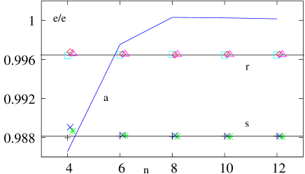
Figure 1: Deviations from the thermodynamic limit ($N_{s}\to\infty$) of three different ideal lattice gases with finite spatial extent for two different values of the ratio $N_{s}/N_{t}$. Some symbols are shifted to the right for clarity. For comparison, the energy density of one of these models is drawn in units of the continuum limit to show the dependence on the cut-off. The data are taken from Table I and II of Ref.bkl . One observes a remarkable cancellation of the UV cut-off effects for $N_{t}>4$ and the emergence of a universal function of $\frac{N_{s}}{N_{t}}$. The horizontal lines are not fits, but denote the two values assumed by the function $1-\frac{15}{2\pi^{2}}(N_{t}/N_{s})^{3}$ as predicted by Eq. (4).

 

Figure 2: Deviation from the thermodynamic limit $f_{\rm SB}$ of the free energy density $f$ of the free gluon gas.

A non-trivial numerical check of the above formulae comes from the mentioned study bkl on $T\to\infty$ limit of $SU(3)$ gauge theory, where three different $O(a^{2})$ and $O(a^{4})$ improved actions were used to explore finite-size effects on ideal lattice gluon gases. The energy density $\epsilon(N_{t}/N_{s},N_{t})$ was evaluated by numerical integration for some values of $N_{t}$ and for two different ratios $N_{s}/N_{t}=4$ and $N_{s}/N_{t}=6$ (5 significant digits) as well as in the thermodynamic limit $\epsilon(0,N_{t})$ (7 significant digits). Their ratios are plotted in Fig.1 as functions of $N_{t}$. In principle, these should be model-dependent functions of $N_{s}/N_{t}$ and $N_{t}$, but there is a remarkable cancellation of the UV cut-off dependence for $N_{t}>4$. As a consequence, there is no other intrinsic length scale in the game besides the size of the system, hence these ratios are expected to collapse toward a universal function of $N_{s}/N_{t}$ which, according to (4), should be $1-\frac{15}{2\pi^{2}}(N_{t}/N_{s})^{3}$. The numerical data fit perfectly this prediction within numerical accuracy.

Let us come to a proof of the main formula (2). For sake of generality, I shall treat the case of a massless scalar field $\phi$ in a (hyper)cubic box of volume $V=L^{D}$ at a temperature $T$. The canonical partition function $Z$ is defined by a functional integral over all periodic field configurations with period $L$ in the space directions and with period $\beta=1/T$ in the imaginary time. The dimensions of the box are large compared to $\beta$, i.e. $LT\gg 1$.

There is a rich literature on a strictly related subject, the Casimir effect, where different methods have been developed to study various kinds of finite-size effects (see e.g. Edery:2005bx for useful formulae and further references). It is however more instructive to account for the functional form of $Z$ by exploiting some simple symmetry principles. First, we require that $Z$ be dimensionless, of course. Owing to the absence of intrinsic length scales, $Z$ should be a function of the unique dimensionless parameter $LT$. This yields invariance under the scale transformation

$$Z=Z(LT)\Leftrightarrow~{}~{}L\to s\,L~{},\beta\to s\,\beta$$ (7)

Secondly, the $D+1$ periodic box defines a cell of an infinite, regular, lattice. The physics should not depend on the choice of the fundamental region tiling the whole $D+1$-dimensional space by discrete translations. This requires modular invariance of the system.

Periodic boundary conditions allow for a zero mode $\phi=\phi_{o}$ of the scalar field. In a system with zero modes the functional integral splits into two factors

$$Z(LT)=C_{o}\,{\cal D}=\,C_{o}\,[{\rm Det}K]^{-\frac{1}{2}}~{},$$ (8)

where $C_{o}$ denotes the zero mode contribution while the other factor is the integral over the Gaussian fluctuations around the zero modes, described by the kinetic operator $K$. The latter can be written as the product over the eigenvalues $\lambda_{k}$ of $K$ in the usual form

$$[{\rm Det}K]^{-\frac{1}{2}}=\prod_{k}^{\prime}\lambda_{k}^{-\frac{1}{2}}~{},$$ (9)

the prime here indicating that we are to exclude the zero eigenvalue. Under general grounds (see e.g.do or we , page 463) one can prove that a rescaling $\lambda_{k}\to s^{-2}\lambda_{k}$ of all non-vanishing eigenvalues yields correspondingly $[{\rm Det}K]^{-\frac{1}{2}}\to s^{{\cal N}}[{\rm Det}K]^{-\frac{1}{2}}$, where ${\cal N}$ denotes the number of zero modes. In the present case $K=-\partial^{2}$ where $\partial^{2}$ is the Laplacian, and

$$\lambda(m_{i},n)=\sum_{i=1}^{D}\left(\frac{2\pi m_{i}}{L}\right)^{2}+\left(\frac{2\pi n}{\beta}\right)^{2}$$ (10)

where the $m_{i}$’s and $n$ run from $-\infty$ to $\infty$. As a consequence, ${\cal D}\equiv[{\rm Det}-\partial^{2}]^{-\frac{1}{2}}$ is a function of $L$ and $\beta$ and the mentioned rescaling property of ${\cal D}$ becomes

$${\cal D}(s\,L,s\,\beta)=\,s\,{\cal D}(L,\beta)~{},$$ (11)

showing that the zero mode factorization (8) spoils the scale invariance of ${\cal D}$. In order to recover the scale invariance of $Z$, the factor $C_{o}$ should have dimensions of length. The only modular invariant quantity with this property can be constructed with the volume of the $D+1$-dimensional cell, namely, $(L^{D}\beta)^{1/(D+1)}$. Choosing $s=1/L$ we get, aside from irrelevant numerical factors,

$$Z=(\beta/L)^{1/(D+1)}\,{\cal D}(1,\beta/L)~{}.$$ (12)

To explicitly evaluate ${\cal D}$ it is convenient to resort to the $\zeta$-function regularization rs ; ha ; dc of the Laplacian determinant

$${\cal D}(1,\beta/L)=\prod_{m_{i},n}^{\prime}\left(\sum_{i=1}^{D}m_{i}^{2}+(LTn)^{2}\right)^{-\frac{1}{2}}~{}.$$ (13)

where the prime now indicates a regularised product. One of the virtues of the $\zeta$ function regularization is that one can deal with regularised sums or products as they were absolutely convergent series and products df ; Gliozzi:1992wa ; Gliozzi:2005cd . In (13) we consider only the factors with $n\not=0$ because the others generate irrelevant numerical constants. It is useful to classify the factors according to the number $k$ of non vanishing $m_{i}$. Denoting with $c_{k}$ the product over the set $\{m_{1}\not=0,\dots m_{k}\not=0,n\not=0\}$ and with $p_{k}$ the product over the set $I_{k}=\{m_{1}>0,\dots m_{k}>0,n>0\}$ we have $c_{k}=p_{k}^{2^{k+1}}$ with

$$p_{k}=\prod_{I_{k}}^{\prime}\left[\sum_{i=1}^{k}m_{i}^{2}+(LTn)^{2}\right]~{},$$ (14)

and

$$\log{\cal D}(1,\beta/L)=-\sum_{k=0}^{D}\left(\matrix{D\cr k}\right)2^{k}\log\,p_{k}~{}.$$ (15)

We now use the $\zeta$-regulated product $\prod_{m>0}^{\prime}m^{2}=2\pi$ to rewrite $p_{k}$ in the form

$$p_{k}=\prod_{I_{k-1}}^{\prime}2\pi\prod_{m>0}\left[1+\frac{\sum_{i=1}^{k-1}m_{i}^{2}+(LTn)^{2}}{m^{2}}\right]~{}.$$ (16)

According to the known formula

$$\prod_{m>0}(1+\frac{\alpha^{2}}{m^{2}})=\frac{e^{\pi\alpha}}{2\pi\alpha}(1-e^{-2\pi\alpha})~{},$$ (17)

we are led to the key identity

$$p_{k+1}=p_{k}^{-\frac{1}{2}}\,e^{L\,E_{C}^{(k)}}\,Q_{k}$$ (18)

with

$$Q_{k}=\prod_{I_{k}}\left[1-e^{-2\pi\sqrt{\sum_{i=1}^{k}m_{i}^{2}+(LTn)^{2}}}\right]~{}.$$ (19)

The $\zeta-$regulated quantity

$$E_{C}^{(k)}=\frac{1}{2}\sum_{I_{k}}^{\prime}\sqrt{\sum_{i=1}^{k}\left(\frac{2\pi m_{i}}{L}\right)^{2}+\left(\frac{2\pi n}{\beta}\right)^{2}}$$ (20)

is the Casimir energy of $\phi$ in a box of size $\frac{\beta}{2}\times(\frac{L}{2})^{k}$ with Dirichlet boundary conditions. Inserting (18) in (15), these Casimir energies combine to form the quantity

$$E_{o}=\sum_{k=0}^{D-1}2^{k}\left(\matrix{D-1\cr k}\right)\,E_{C}^{(k)}~{}.$$ (21)

This is the zero-point energy of the massless scalar field in the periodic box of size $\beta\times L^{D-1}$, which is exactly known even at finite values of $LT$ (see e.g.Edery:2005bx ):

$$E_{o}=-\frac{L^{D-1}}{\beta^{D}}\frac{\Gamma(\frac{D+1}{2})}{\pi^{\frac{D+1}{2}}}\,\zeta(D+1)~{},$$ (22)

where $\zeta(x)$ is the Riemann zeta function. Applying this to Eq. (15) and defining

$$\log Q=\sum_{k=0}^{D-1}2^{k+1}\left(\matrix{D-1\cr k}\right)\,\log\,Q_{k}\simeq e^{-2\pi LT}+\dots$$ (23)

we may rewrite Eq.(12) in the form

$$\log Z=\frac{L^{D}}{\beta^{D}}\frac{\Gamma(\frac{D+1}{2})}{\pi^{\frac{D+1}{2}}}\zeta(D+1)-\frac{\log\frac{L}{\beta}}{D+1}-\log Q\,.$$ (24)

This is the final result. It can be rewritten in a more evocative form

$$\log Z=-L\,E_{o}-\frac{\log LT}{D+1}-\sum_{\vec{k}}\log(1-e^{-L\omega_{\vec{k}}})~{},$$ (25)

where $Z$ can now be viewed as the canonical partition function of $\phi$ in the asymmetric, periodic, box $L^{D-1}\beta$ in equilibrium at the “temperature” $1/L$; the sum is over the momenta of the normal modes of energy $\omega_{\vec{k}}$. The rotation, or modular transformation, of the fundamental $D+1$ cell with respect to the standard approach to blackbody radiation has made it possible to highlight the finite size effects of $\log Z$. Aside from small exponential corrections, it differs from the thermodynamic limit by a non-negligible logarithmic term. The latter is essential to enforce modular invariance, which was obvious at the beginning of the calculation. Its origin can be traced to the zero mode subtraction in Eq.(8).

When $D=1$ we recover the known partition function of a scalar massless boson on a 2-torus. Of course, for a free gluon gas one has to multiply this result by the number of polarisation states and by the dimensions of the adjoint representation of the gauge group.

In conclusion, in this paper it has been pointed out that the free energy of an ideal gluon gas in a periodic box is affected by non-negligible IR finite-size effects. It would be very interesting to observe similar effects in the interacting case. Unfortunately, in order to see them varying the ratio $T/T_{c}$ by acting on the coupling constant does not suffice: one has to modify the ratio $N_{s}/N_{t}=LT$. Notice that the finite-size deviation of $f$ does not influence only the evaluation of the pressure but also the internal energy and the entropy. In fact in lattice simulations one calculates two different physical quantities: the trace anomaly $\Delta=\epsilon-3p$ and the free energy density $f$, and one defines the energy density as $\epsilon\simeq\Delta-3f$ and the entropy density as $s\simeq(\Delta-4f)/T$; in view of Eq.(6) these are true only in the thermodynamic limit. It has been observed bb that the cut-off dependence in $\Delta$ is much smaller than for the pressure alone. This could be a clue to IR finite-size effects.

References

- (1) P. Arnold and C. Zhai, Phys. Rev. D 50 7603 (1994) [arXiv:hep-ph/9408276], ibid. 51, 1906 (1995) [arXiv:hep-ph/9410360]; C. Zhai and B. Kastening, ibid. 52, 7232 (1995) [arXiv:hep-ph/9507380].
- (2) E. Braaten and A. Nieto, Phys. Rev. D 53, 3421 (1996) [arXiv:hep-ph/9510408].
- (3) K. Kajantie, M. Laine, K. Rummukainen and Y. Schröder, Phys. Rev. D 67, 105008 (2003) [arXiv:hep-ph/0211321].
- (4) A. Hietanen, K. Kajantie, M. Laine, K. Rummukainen and Y. Schröder, JHEP 01, 013 (2005) [arXiv:hep-lat/0412008].
- (5) F. Di Renzo, M. Laine, V. Miccio, Y. Schröder and C. Torrero, JHEP 07, 026 (2006) [arXiv:hep-ph/0605042].
- (6) G. Boyd, J. Engels, F. Karsch, E. Laermann, C. Legeland, M. Lutgemeier and B. Petersson, Nucl. Phys. B 469, 419 (1996) [arXiv:hep-lat/9602007].
- (7) J. Engels et al, Phys. Lett. B 396, 210 (1997) [arXiv:hep-lat/9612018].
- (8) F. Karsch, E. Laermann and A. Peikert, Phys. Lett. B 478, 447 (2000) [arXiv:hep-lat/0002003].
- (9) C. Bernard et al., arXiv:hep-lat/0611031.
- (10) B. Bringoltz and M. Teper, Phys. Lett. B 628, 113 (2005) [arXiv:hep-lat/0506034].
- (11) B. Beinlich, F. Karsch and E. Laermann, Nucl. Phys. B 462, 415 (1996) [arXiv:hep-lat/9510031].
- (12) J. Engels, J. Fingberg, F. Karsch, D. Miller and M. Weber, Phys Lett. B 252, 625 (1990).
- (13) A. Edery, J. Phys. A 39, 685 (2006) [arXiv:math-ph/0510056].
- (14) J. S. Dowker, Phys. Rev. D 37, 558 (1988).
- (15) S. Weinberg The Quantum Theory of Fields Vol.II, Cambridge University Press 1996.
- (16) D. B. Ray and I. M. Singer, Adv. Math. 7, 145 (1971).
- (17) S. W. Hawking, Commun. Math. Phys. 55, 133 (1977).
- (18) J. S. Dowker and R. Critchley, Phys. Rev. D 13, 3224 (1976).
- (19) K. Dietz and T. Filk, Phys. Rev. D 27, 2944 (1982).
- (20) F. Gliozzi, Acta Phys. Polon. B 23, 971 (1992) [arXiv:hep-lat/9210007].
- (21) F. Gliozzi, Nucl. Phys. Proc. Suppl. 153, 120 (2006) [arXiv:hep-lat/0511039].