2+1 flavor domain wall QCD on a (2 fm)³ lattice:
light meson spectroscopy with $L_{s}$ = 16

Abstract

We present results for light meson masses and pseudoscalar decay constants from the first of a series of lattice calculations with 2+1 dynamical flavors of domain wall fermions and the Iwasaki gauge action. The work reported here was done at a fixed lattice spacing of about 0.12 fm on a $16^{3}\times 32$ lattice, which amounts to a spatial volume of (2 fm)³ in physical units. The number of sites in the fifth dimension is 16, which gives $m_{\rm res}=0.00308(4)$ in these simulations. Three values of input light sea quark masses, $m_{l}^{\rm sea}\approx 0.85\,m_{s},0.59\,m_{s}$ and $0.33\,m_{s}$ were used to allow for extrapolations to the physical light quark limit, whilst the heavier sea quark mass was fixed to approximately the physical strange quark mass $m_{s}$. The exact rational hybrid Monte Carlo algorithm was used to evaluate the fractional powers of the fermion determinants in the ensemble generation. We have found that $f_{\pi}=127(4)$ MeV, $f_{K}=157(5)$ MeV and $f_{K}/f_{\pi}=1.24(2)$, where the errors are statistical only, which are in good agreement with the experimental values.

I Introduction

The successful determination of the light hadron spectrum serves as an important test of lattice QCD. With the emergence of powerful computers and new algorithms, lattice QCD has entered an era of dynamical simulations where two light quarks and one strange quark are included in the vacuum polarization effects. (These simulations are referred to as 2+1 flavor simulations.) Since current simulations use light quarks that are heavier than the physical values, extrapolations to the light quark region are still required, and having control of these extrapolations is vital for a comparison with experimental results. Chiral perturbation theory provides a framework for such extrapolations, although the range of quark masses for which a given order of chiral perturbation theory is accurate is still under investigation.

Symmetry plays an important role in hadron physics. The domain wall fermion (DWF) formulation Kaplan (1992); Shamir (1993); Furman and Shamir (1995) respects flavor symmetry and has approximate chiral symmetry, with the introduction of an auxiliary fifth dimension. When the extent of this fifth dimension, denoted as $L_{s}$, goes to infinity, chiral symmetry is fully recovered. In addition, unlike Wilson and staggered fermions, domain wall fermions (and the closely connected overlap fermions) allow chiral symmetry to be recovered at finite lattice spacing. While certainly an important improvement for the light hadron spectrum calculation presented here, this good chiral symmetry is vital for accurate operator renormalization and control of operator mixing in a wide variety of important hadronic matrix elements. As evidenced by existing work in quenched QCD, the chiral properties of domain wall fermions make calculations possible that cannot currently be done with other formulations Blum et al. (2003); Noaki et al. (2003). To move beyond the quenched approximation, 2+1 flavor ensembles are needed. The production of these ensembles and the determination of their basic properties are important steps towards the goal of measuring a wide variety of physically interesting quantities using this formulation and are the focus of this paper.

In practice, $L_{s}$ is taken to be on the order of 10-20 sites so that some residual chiral symmetry breaking remains. However, this residual chiral symmetry breaking is highly suppressed. Compared to Wilson fermions where the residual chiral symmetry breaking is an ${\cal O}(1)$ effect, for DWF it is of ${\cal O}(10^{-3})$ or smaller, depending on the size of $L_{s}$. To leading order in the lattice spacing $a$, the only effect of this residual chiral symmetry breaking is a simple mass renormalization (denoted by $m_{\rm res}$) added to the input quark mass. Additional chiral symmetry breaking effects enter at higher order in $a$, but they are suppressed by the additional powers of $a$ and also vanish as $L_{s}$ becomes large. This situation simplifies the chiral extrapolation of physical observables, and allows us to study those aspects of hadron phenomenology where chiral symmetry is important with reduced systematic uncertainties.

Domain wall fermions are both on- and off-shell improved, since for any quantity a traversal of the fifth dimension is required to mix chiralities. Such a traversal is suppressed for large $L_{s}$, a suppression which gives rise to the small value for $m_{\rm res}$ and which depends on $L_{s}$ as $\exp(-\alpha L_{s})$ if the generic, weak coupling behavior of residual chiral symmetry breaking effects is used Golterman and Shamir (2005). Thus, the resulting theory is accurate up to terms of ${\cal O}(a\exp(-\alpha L_{s}))$ and ${\cal O}(a^{2})$.

For amplitudes which violate chiral symmetry by two units, a suppression of order $m_{\rm res}^{2}$ or $\exp(-2\alpha L_{s})$ is expected. This estimate may fail in the case of composite operators with many fields at the same space-time pointGolterman and Shamir (2005), where one must give special consideration to chiral symmetry breaking arising from rare, localized modes that are undamped in the fifth dimension. However, the detailed flavor structure of the operator must be considered which, in important cases, prevents these localized modes from contributing Christ (2005). The result is that chirally disallowed operator mixings are generally under good control with DWF at finite $L_{s}$.

For power divergent quantities, one finds that if an operator receives an $m_{f}/a^{n}$ contribution, where $m_{f}$ is the quark mass, then for finite $L_{s}$ it will generally receive an ${\cal O}(m_{\rm res})/a^{n}$ contribution Blum et al. (2004). Because the residual chiral symmetry breaking is entering a divergent amplitude, it will not be determined by the chiral symmetry breaking at low energies described by $m_{\rm res}$. However, it will be of this order, as has been demonstrated in Blum et al. (2003). Thus, for such quantities the simple replacement $m_{f}/a^{n}\rightarrow(m_{f}+m_{\rm res})/a^{n}$ provides a sensible estimate of but not an accurate value for the effects of residual symmetry breaking on the quantity in question. For example, such a term enters the chiral condensate $\langle\bar{q}q\rangle$. This implies that to compute $\langle\bar{q}q\rangle$ with domain wall fermions an extrapolation to large $L_{s}$ must be made or that this physical quantity should be determined from the density of Dirac eigenvalues at zero, so that ultraviolet chiral symmetry breaking effects do not enter. In contrast, a similar, uncertain ${\cal O}(m_{\rm res}/a^{2})$ term which appears in the matrix elements of the weak interaction operator $O_{6}$, does not effect the quantity of interest which is proportional to $m_{f}$ Blum et al. (2003). For a more complete discussion of the effects of residual chiral symmetry breaking for domain wall fermion see, for example, Refs Furman and Shamir (1995); Blum et al. (2004, 2002, 2003).

These benefits of controlled chiral symmetry breaking must be weighed against the computing cost for domain wall fermions, which are naively ${\cal O}(L_{s})$ more expensive than conventional fermion formulations Clark (2006). In balance, we believe that the benefits of domain wall fermions outweigh their extra numerical costs, because of the much larger range of observables that are accessible to this formulation.

Studies which established a set of parameter values suitable for 2+1 flavor simulations with domain wall fermions were reported in Antonio et al. (2006a). In the present paper we describe the first of a series of 2+1 flavor DWF simulations which use the parameters as determined in Antonio et al. (2006a), and explore in detail the systematic effects arising in such a full dynamical simulation with domain wall fermions. Specifically, we use the Iwasaki gauge action with gauge coupling $\beta=2.13$ on a lattice of $16^{3}\times 32$, which gives a lattice spacing of about 0.12 fm and a spatial lattice extent of about 2 fm. This volume should be large enough to give accurate results for the physics of the pseudoscalar mesons simulated here: those with a mass ratio to vector meson masses in the range $0.5\leq m_{P}/m_{V}\leq 1.0$. Larger volume simulations at the same coupling using lighter quark masses are underway, as are simulations at weaker couplings, also with lighter quark masses. The volumes used in the work presented here do not allow lighter dynamical quark masses to be used, so the full benefits of DWF will not be visible. However, the current simulations allow us to demonstrate that more costly simulations at larger volumes and lighter quark masses are feasible. Since baryonic observables may suffer from non-negligible finite volume effects in the current volume, we will only focus on light meson physics in this paper. In particular, we will present results for light pseudoscalar meson masses and decay constants, and calculate quantities of direct phenomenological interest, such as the light quark masses and $f_{K}/f_{\pi}$.

One of the many complexities of 2+1 flavor simulations is the presence of the fractional powers of the fermion determinants in the path integral, which the conventional hybrid Monte Carlo algorithm is not able to evaluate. We employed the rational hybrid Monte Carlo (RHMC) algorithm by Clark and Kennedy Clark and Kennedy (2004); Clark et al. (2005, 2006), which is not only free of finite step size errors, but also has proved to be quite efficient after recent improvements and tunings Antonio et al. (2006b). The gauge configurations used in this work were mainly generated with one variant of the RHMC algorithm. We describe the details of this algorithm in Section II. The algorithm was further improved after the major part of this work had been done. It is thus to our advantage to study how the computing cost and ensemble properties change with the new improvements. We compare these two variants of the RHMC algorithm in Section VI.

This paper is organized as follows. In Section II we present the details of generation of the gauge configurations using the RHMC algorithm. We discuss the thermalization and autocorrelations of the ensembles in Section III. Section IV gives the results of the light meson masses and decay constants, including the residual chiral symmetry breaking in these simulations. The results for physical observables in the chiral limit are presented in Section V. Section VI discuses an extension of one of the ensembles using an improved RHMC algorithm. Our conclusions are given in Section VII.

II Generation of Gauge Configurations

In this study we have used the Iwasaki renormalization-group improved gauge action and $2+1$ flavors of dynamical domain wall fermions; details of the action and our notation may be found in Antonio et al. (2006a). Our ensembles were generated using two new variants of the RHMC algorithm as described below.

For the case of two degenerate light quarks of mass, $m_{l}$, and a strange quark of mass, $m_{s}$, integrating out the fermion fields in the path integral leads to

$$\frac{\det\left[D_{\rm DWF}^{\dagger}(M_{5},m_{l})D_{\rm DWF}(M_{5},m_{l})\right]}{\det\left[D_{\rm DWF}^{\dagger}(M_{5},1)D_{\rm DWF}(M_{5},1)\right]}\;\;\frac{\det^{1/2}\left[D_{\rm DWF}^{\dagger}(M_{5},m_{s})D_{\rm DWF}(M_{5},m_{s})\right]}{\det^{1/2}\left[D_{\rm DWF}^{\dagger}(M_{5},1)D_{\rm DWF}(M_{5},1)\right]}$$ (1)

where $D_{\rm DWF}(M_{5},m)$ is the domain wall Dirac operator, $M_{5}$ is the height of the domain wall, and $m$ is the fermion mass. The determinants in the denominator arise from the Pauli-Villars fields introduced to cancel the bulk infinity which arises as the size of the fifth dimension $L_{s}\to\infty$.

We may use the identity $\det(M)=[\det^{1/n}(M)]^{n}$ to simulate various different decompositions of the same fermionic determinants using RHMC. If we adopt the shorthand notation ${\cal D}(m_{i})=D_{\rm DWF}^{\dagger}(M_{5},m_{i})D_{\rm DWF}(M_{5},m_{i})$, we may write the ratio of determinants in Eq. (1) as

$$\frac{\det^{1/2}[{\cal D}(m_{l})]\;\det^{1/2}[{\cal D}(m_{l})]\;\det^{1/2}[{\cal D}(m_{s})]}{\det[{\cal D}(1)]\;\det^{1/2}[{\cal D}(1)]}.$$ (2)

In our previous paper Antonio et al. (2006a), each determinant in Eq. (2) was associated with a separate pseudo-fermion field, and a standard RHMC algorithm Kennedy et al. (1999); Clark and Kennedy (2006) was employed.

The pseudo-fermion action for molecular dynamics evolution of a single quark flavor of mass $m$ takes the form $S_{\rm pf}=\phi^{\dagger}{\cal D}^{-1/2}(m)\phi$. We may improve the efficiency of RHMC by taking advantage of the properties of the expansion coefficients in the partial-fraction formulation of the $p^{\rm th}$-order rational approximation, $x^{-1/2}\simeq\left\{\alpha_{0}+\sum_{k=1}^{p}\frac{\alpha_{k}}{x+\beta_{k}}\right\}$. The “shifts”, $\beta_{k}$, which are all real and positive, are ordered according to increasing magnitude, and the $\alpha_{k}$ are all real and positive. The fermion force is

$$-S^{\prime}_{\rm pf}=\sum_{k=1}^{p}\alpha_{k}\,\phi^{\dagger}\left({\cal D}(m)+\beta_{k}\right)^{-1}{\cal D}^{\prime}(m)\left({\cal D}(m)+\beta_{k}\right)^{-1}\phi\,,$$ (3)

where the prime denotes differentiation with respect to the gauge field. Somewhat remarkably, the inverses with the smallest shifts, $\beta_{k}$, which are the most expensive to evaluate, are associated with the smallest residues $\alpha_{k}$, and thus lead to relatively-small contributions to the fermion force Clark and Kennedy (2006); Clark et al. (2006). It is then natural to split the sum in Eq. (3) into two parts: “light poles” with $1\leq k\leq r$, and “heavy poles” with $r<k\leq p$, and evaluate their contributions to the fermion force on different timescales using a Sexton-Weingarten multi-timescale integrator Sexton and Weingarten (1992). The light-pole contributions are evaluated only on the largest timescale, the heavy poles on an intermediate timescale, and the gauge fields on the finest timescale.

Table 1: Parameter values for $2+1$ flavor RHMC runs on $16^{3}\times 32$ lattices with $L_{s}=16$, $M_{5}=1.8$, $\beta=2.13$, $m_{s}^{\rm sea}=0.04$. $N_{\rm MD\;units}$ is the number of molecular dynamics time units obtained from an ordered start, except for the $m_{l}^{\rm sea}=0.03$ ensemble generated using RHMC II, which started from the last configuration generated using RHMC I. $N_{\rm step1}$ is the number of coarse integration steps of size $\delta\tau$ per MD time unit. The intermediate integration scale is $\delta\tau/N_{\rm step2}$ and the finest scale is $\delta\tau/(N_{\rm step2}\,N_{\rm step3})$. The RHMC acceptance rate is given in the second last column. The final column denotes the variant of the RHMC algorithm used.

$m_{l}^{\rm sea}$	$N_{\rm MD\;units}$	$\delta\tau$	$N_{\rm step1}$	$N_{\rm step2}$	$N_{\rm step3}$	Acc	Alg
0.01	4015	0.13	8	2	8	70%	RHMC I
0.02	4045	0.14	7	2	8	56%	RHMC I
0.03	4020	0.14	7	2	8	57%	RHMC I
0.03	3580	0.25	4	1	6	80%	RHMC II

In order to maximize the acceptance rate per unit computational cost, we optimized the order of the rational approximations and the points, $r$, at which the partial-fraction sums are split, whilst also varying the three Sexton-Weingarten timescales. The optimal rational approximations and splits were $(p,r)=(10,4)$ for the light quarks, $(p,r)=(10,3)$ for the strange quark, and $(p,r)=(6,1)$ for the Pauli-Villars field associated with the strange quark.

In the RHMC accept/reject step, we used rational approximations of order $16$ and $9$, respectively, for the quark and Pauli-Villars fields.

For all ensembles, we used the second-order minimum-norm (2MN) integrator Sexton and Weingarten (1992); Omelyan and Folk (2003); Takaishi and de Forcrand (2006); Urbach et al. (2006) with approximately unit-length trajectories. We tuned the free parameter in 2MN to $\lambda=0.22$ to minimize the RMS change in the Hamiltonian, $\langle(\Delta H)^{2}\rangle^{1/2}$, along a set of RHMC trajectories.

This completes the description of the RHMC I algorithm used to generate the ensembles in the main part of this work. We used three values of $m_{l}$ to generate the gauge configurations using this algorithm, with $m_{s}$ fixed to 0.04 (in lattice units). Further parameters and simulation details are given in Table 1.

Recently, we developed a more efficient implementation, RHMC II, which was used to generate the additional ensemble discussed in Section VI. Following Aoki et al Aoki et al. (2005) one may employ a single pseudo-fermion field to estimate directly each ratio of determinants in Eq. (1). This reduces the stochastic noise in the molecular dynamics evolution and speeds up the calculation because a larger step size can be used in the integration. Furthermore, we can rewrite the ratio of fermion determinants as

$$\det\left\{\frac{{\cal D}(m_{l})}{{\cal D}(1)}\right\}\;\det\left\{\frac{{\cal D}(m_{s})}{{\cal D}(1)}\right\}^{1/2}=\det\left\{\frac{{\cal D}(m_{l})}{{\cal D}(m_{s})}\right\}\;\det\left\{\frac{{\cal D}(m_{s})}{{\cal D}(1)}\right\}^{1/2}\;\det\left\{\frac{{\cal D}(m_{s})}{{\cal D}(1)}\right\}^{1/2}\;\det\left\{\frac{{\cal D}(m_{s})}{{\cal D}(1)}\right\}^{1/2},$$ (4)

thus preconditioning the light quark Dirac operator by the strange quark Hasenbusch and Jansen (2003); Urbach et al. (2006). We associate the first determinant on the RHS of Eq. (4) with a single pseudo-fermion field, and introduce separate pseudo-fermion fields for each of the three “strange quarks” in the rest of the determinants on the RHS. Again we used a multiple-timescale integrator, with the preconditioned light quarks using the largest step size, the strange/Pauli-Villars fields an intermediate size, and the gauge fields the finest size. The optimal free parameter of the MN2 integration scheme was found to be $\lambda=0.22$ in this case. The relevant parameters are also given in Table 1.

To distinguish the valence quark masses from the sea quark masses, we will use $m_{l}^{\rm sea}$ to denote the light dynamical quark masses, and $m_{1}$ and $m_{2}$ to denote the masses of two valence quarks that make up a meson. Whenever a meson is composed of two degenerate quarks, a short-hand notation $m_{\rm val}$ may be used to refer to the mass of each component quark. We use the lattice units for various quantities throughout the paper, unless physical units are explicitly given.

III Thermalization and Autocorrelations

In this section we will discuss the thermalization and autocorrelations of the ensembles which build a foundation for the data analysis of various quantities. For most of our measurements, we discarded the first 500 molecular dynamics time units to account for the thermalization of the gauge fields. Shown in Figure 1 is the evolution history of the plaquette for all three ensembles. The straight lines are the average values of the plaquette for each ensemble from time unit 2000 to 4000. It is evident that the gauge fields have come to equilibrium after ${\cal O}(500)$ molecular dynamics time units. We have also measured the chiral condensate $\left<\overline{q}q\right>$ through a stochastic estimator with one single hit for the first 3000 molecular dynamics time units, starting from time unit 500, and found no signs of further equilibration (Figure 2). This supports our choice of cut to allow for the thermalization of the ensemble.

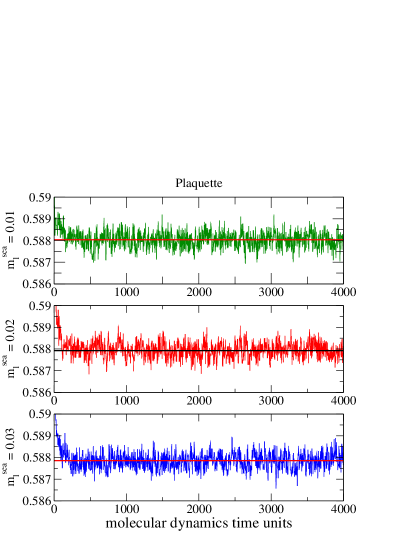
Figure 1: Evolution history of the plaquette for all three ensembles, measured every MD time unit. The straight lines are the averages from trajectory 2000 to 4000 for each ensemble.

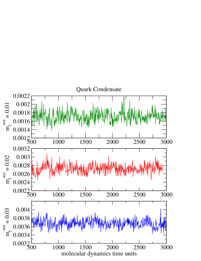
Figure 2: Evolution history of the quark condensate $\left<\overline{q}q\right>$ for the first 3000 molecular dynamics time units at three dynamical points: $m_{\rm val}=m_{l}^{\rm sea}=0.01$ (top), $m_{\rm val}=m_{l}^{\rm sea}=0.02$ (middle) and $m_{\rm val}=m_{l}^{\rm sea}=0.03$ (bottom). The measurements were taken every 5 molecular dynamics time units.

To obtain reliable estimates for the statistical errors in the physical observables, we also investigate the autocorrelations in the ensembles. While the autocorrelation time may differ from quantity to quantity, we calculate the autocorrelations for the quantities of our direct interest, such as meson correlation functions. We adopted the same method as in Aoki et al. (2005) and calculated the integrated autocorrelation time, $\tau_{\rm int}$, for the two-point pseudoscalar correlation function at time slice 12 obtained from a Coulomb gauge fixed wall source at $t=0$ with two degenerate valence quarks with $m_{\rm val}=0.01$ for the $m_{l}^{\rm sea}=0.01$ ensemble, where the correlation function was measured every 5 molecular dynamics time units. This is shown in Figure 3. We can see that the integrated autocorrelation time reaches a plateau of about 20 to 25 time units. The separation between two independent measurements is then about $2\tau_{\rm int}\approx 50$ molecular dynamics time units. Thus we chose to average the data over a block of measurements in such a way that the span of the measurements in each block covers at least 50 molecular dynamics time units whenever possible prior to the standard jackknife analysis.

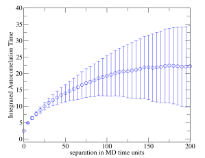
Figure 3: Integrated auto-correlation time for the pseudoscalar two-point correlation function at time slice 12 with $m_{l}^{\rm sea}=m_{\rm val}=0.01$.

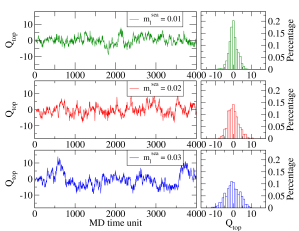
Figure 4: The topological charge as measured by gluonic fields on the three ensembles. The left three panels are the topological charge as a function of the molecular dynamics time. Each of the three graphs on the right represents the normalized histogram of the corresponding topological charge evolution on the left.

The evolution of the topological charge is another indicator of how fast the gauge fields decorrelate. On each ensemble we measured the topological charge using the classically ${\cal O}(a^{2})$ improved definition of the field tensor as defined in Antonio et al. (2006a). Figure 4 shows that the gauge field moves frequently between different topological charge sectors. Also shown in Figure 4 are the histograms of the topological charge, which indicate that different topological sectors are sampled reasonably well. However, it is also worth noting that correlations on a scale of a few hundred molecular dynamics time units are present in the $m_{l}^{\rm sea}=0.03$ ensemble. This may imply that the value for the autocorrelation time discussed in the previous paragraph is under-estimated. Ideally we should use a larger block size prior to the jackknife analysis to have more robust error estimates, but we are constrained by the moderate lengths of the simulations and have chosen to use a block size that is not too small, but at the same time leaves a reasonable number of jackknife blocks to perform covariant fits when necessary.

IV Hadronic Observables

IV.1 Calculation Details and Fitting Procedures

We used several different source and sink operators to calculate the quark propagators needed for the two-point correlation functions. To be specific, we used a local operator (denoted as L), a Coulomb gauge fixed wall operator (denoted as W), and a Gaussian smeared operator Allton et al. (1993) (denoted as G), for the source and/or sink, in an attempt to investigate the systematic uncertainties coming from excited-state contamination. Here we adopt the same notation as in Antonio et al. (2006a) and denote the types of meson correlation functions by the different source and sink operators used in the quark propagators. For example, GL-GL means a correlation function composed of two quark propagators, each of which is computed using the Gaussian smeared source operator and the local sink operator. The sources are placed at multiple locations to reduce the short-term noise induced by the fluctuations in the gauge fields. The correlation functions are averaged over different source locations before the standard jackknife analysis is performed. Details of the calculation parameters are tabulated in Tables 2 and 3.

Table 2: Measurement parameters for the WL-WL correlation functions for all the three ensembles. $m_{l}^{\rm sea}$ denotes the light sea quark mass. $m_{1}$ and $m_{2}$ denote the two valence quarks composing the mesons. $\Delta$ is the separation between measurements in molecular dynamics time units.

$m_{l}^{\rm sea}$	$m_{1}$	$m_{2}$	range	$\Delta$	$N_{\rm meas}$	$t_{\rm src}$
0.01	0.01	0.01	500 - 3995	5	700	0, 16
0.01	0.02	0.02	500 - 3995	5	700	0, 16
0.01	0.03	0.03	500 - 3995	5	700	0, 16
0.01	0.04	0.04	500 - 3995	5	700	0, 16
0.02	0.01	0.01	500 - 4045	5	710	0, 16
0.02	0.02	0.02	500 - 4045	5	710	0, 16
0.02	0.03	0.03	500 - 4045	5	710	0, 16
0.02	0.04	0.04	500 - 4045	5	710	0, 16
0.03	0.01	0.01	500 - 3995	5	700	0, 16
0.03	0.02	0.02	500 - 3995	5	700	0, 16
0.03	0.03	0.03	500 - 3995	5	700	0, 16
0.03	0.04	0.04	500 - 3995	5	700	0, 16

Table 3: Measurement parameters for the LL-LL, GG-GG and GL-GL correlation functions for all the three ensembles. $m_{l}^{\rm sea}$ denotes the light sea quark mass. $m_{1}$ and $m_{2}$ denote the two valence quarks composing the mesons. $\Delta$ is the separation between measurements in molecular dynamics time units.

$m_{l}^{\rm sea}$	$m_{1}$	$m_{2}$	range	$\Delta$	$N_{\rm meas}$	$t_{\rm src}$
0.01	0.01	0.01	500 - 3990	10	350	0, 16
0.01	0.01	0.04	500 - 3990	10	350	0, 16
0.01	0.04	0.04	500 - 3990	10	350	0, 16
0.01	0.01	0.01	505 - 3995	10	350	8, 24
0.01	0.01	0.04	505 - 3995	10	350	8, 24
0.01	0.04	0.04	505 - 3995	10	350	8, 24
0.02	0.02	0.02	500 - 3990	10	350	0, 16
0.02	0.02	0.04	500 - 3990	10	350	0, 16
0.02	0.04	0.04	500 - 3990	10	350	0, 16
0.02	0.02	0.02	505 - 3995	10	350	8, 24
0.02	0.02	0.04	505 - 3995	10	350	8, 24
0.02	0.04	0.04	505 - 3995	10	350	8, 24
0.03	0.03	0.03	500 - 3990	10	350	0, 16
0.03	0.03	0.04	500 - 3990	10	350	0, 16
0.03	0.04	0.04	500 - 3990	10	350	0, 16

In parallel to the spectrum calculations, we have also done another set of measurements necessary for the extraction of weak matrix elements (see, for example, Ref. Blum et al. (2003)), in which the quark propagators were calculated from Coulomb gauge fixed wall sources at time slices $t_{\rm src}=5$ and $t_{\rm src}=27$. In contrast to the standard spectrum measurement, here the meson correlation functions were constructed from the sum of propagators computed with periodic (P) and anti-periodic (A) boundary conditions in the time direction. This has the effect of doubling the temporal extent of the lattice which gives a longer time range to extract the meson masses. Five different valence masses are used to compute the quark propagators and the meson correlation functions are constructed from all possible combinations of these propagators. The details of measurements are given in Table 4. We will use “P+A” to refer to the results obtained from these data sets hereafter.

Table 4: Measurement parameters for the correlation functions measured with P+A boundary conditions for all the three ensembles. $m_{l}^{\rm sea}$ denotes the light sea quark mass. $m_{1}$ and $m_{2}$ denote the two valence quarks composing the mesons. $\Delta$ is the separation between measurements in molecular dynamics time units.

$m_{l}^{\rm sea}$	$m_{1}$	$m_{2}$	range	$\Delta$	$N_{\rm meas}$	$t_{\rm src}$
0.01	0.01 - 0.05	0.01 - 0.05	1000 - 4000	20	150	5, 27
0.02	0.01 - 0.05	0.01 - 0.05	1000 - 4000	20	150	5, 27
0.03	0.01 - 0.05	0.01 - 0.05	1000 - 4000	20	150	5, 27

To get the meson masses and the corresponding amplitudes of the correlation functions, we performed the standard covariant $\chi^{2}$ fits to the correlation functions using the hyperbolic cosine form:

$$C(t)=A\left[e^{-m_{G}t}+e^{-m_{G}(T-t)}\right]$$ (5)

where $m_{G}$ is the ground-state meson mass, and $t$ is the time slice relative to the source. Note that here $T$ is the extent in the time direction of the lattice, i.e. 32 for the standard spectrum measurements and 64 for the P+A measurements. This relation assumes that the separation between the source and sink operators is large enough that the contamination from the excited states is negligible. However, different source operators have different degrees of overlap with excited states, and hence the minimum time slice that should be included in each fit may differ. To reduce the uncertainties in fit parameters from the choice of fit range, we also performed simultaneous fits to two types of correlation functions using a double-cosh form which give both the ground-state and the first-excited-state meson masses. We found that the ground-state meson masses obtained from the double-cosh fits were consistent with the simple cosh fit in Eq.(5). Since we are mostly interested in the ground-state meson masses in this paper, we will only present results obtained from the single cosh fits unless otherwise stated.

In order to determine a proper fit range for the meson masses using Eq.(5), we examined the effective masses as defined by

$$m_{\rm eff}={\rm cosh}^{-1}\left[\frac{C(t+1)+C(t-1)}{2C(t)}\right]$$ (6)

and chose the minimum time slice in the fit to be the onset of the plateau in the effective mass. A more stringent way to determine the best fit range is to check how the mass obtained from the fit and the resulting $\chi^{2}$/dof vary with the fit range. Since the fits are insensitive to the maximum time slice used, we only investigated the variations with respect to the lower bound (denoted as $t_{\rm min}$) and fixed the upper bound (denoted as $t_{\rm max}$) to $T/2$ for the GL-GL and WL-WL data sets. In Figure 5, the fitted masses and $\chi^{2}$/dof for the pseudoscalar correlation functions are plotted for each light dynamical point with $m_{\rm val}=m_{l}^{\rm sea}$. As we can see, the central values of the fitted masses are insensitive to the choice of $t_{\rm min}$ when $t_{\rm min}$ is above 8 or 9 for both GL-GL and WL-WL data sets. To obtain high confidence level for the fits, we also seek to have minimal $\chi^{2}$/dof in the time range where the fits are stable.

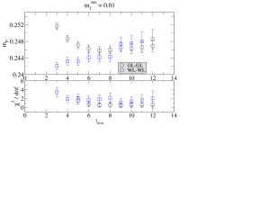
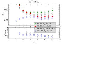
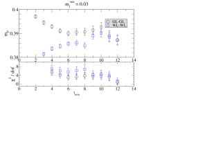
Figure 5: Variation of the pseudoscalar masses obtained from the correlated fits and the corresponding $\chi^{2}$/dof with respect to $t_{\rm min}$ for each of the dynamical points.

Typically the fitted pseudoscalar meson masses from WL-WL and GL-GL correlation functions agree quite well when $t_{\rm min}$ is above 9. An exception is the $m_{l}^{\rm sea}=0.02$ data set, where results from GL-GL correlation functions are larger than those from WL-WL correlation functions by a few standard deviations. The deviations result from the fact that the GL-GL measurements were performed at an additional set of source locations which were not used in the WL-WL measurements. When only the data with the source operator at time slices 0 and 16 are included in the analysis, the results obtained from GL-GL and WL-WL agree within statistical uncertainties, whilst the GL-GL measurements from sources at time slices 8 and 24 give much larger values. Hence when all the sources are combined in the analysis, the values of the fitted masses are much higher from the GL-GL correlators than those from the WL-WL correlators. The fact that the results are so sensitive to the different source locations indicates that we have not sampled phase space extremely well. Thus, the errors obtained from the standard jackknife procedure may be under-estimated.

IV.2 Meson Masses

The pseudoscalar meson masses can be obtained from several different correlation functions Blum et al. (2004); Antonio et al. (2006a). We will show the results from both the pseudoscalar (PP) and axial vector (AA) channels. The effective masses in the pseudoscalar channel at the light dynamical points for all three ensembles are shown in Figure 6. The effective masses from LL-LL correlation functions typically have later approaches to plateaus and leave us with fewer time slices to perform the fits. Thus we will not quote results from these data sets unless otherwise noted. We also note that there are some variations in the effective masses greater than estimates of the standard deviation from the variance of the data. The presence of these variations with 4000 MD time units may be another indication of long-term autocorrelations in these ensembles. Although we do not fully understand the cause of this problem, it is likely due to the algorithm we used to generate these gauge configurations. This will be further addressed in Section VI.

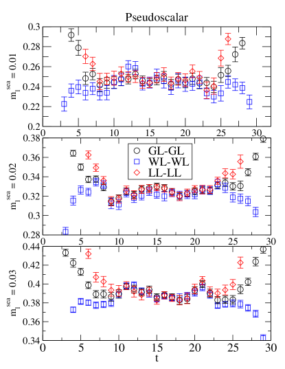
Figure 6: Pseudoscalar effective masses from WL-WL, LL-LL and GL-GL correlation functions for the three ensembles. The valence quarks are degenerate, with the masses equal to the light sea quark mass of that ensemble.

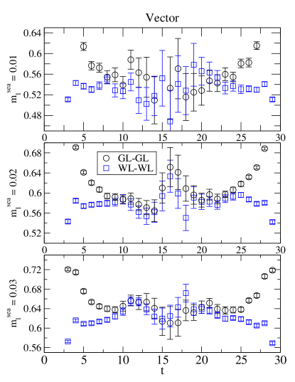
Figure 7: Vector effective masses from WL-WL and GL-GL correlation functions for the three ensembles. The valence quarks are degenerate, with the masses equal to the light sea quark mass of that ensemble.

We determined the vector meson masses by averaging over the three polarizations to reduce statistical fluctuations. Some representative effective masses for the vector mesons are shown in Figure 7. They are typically noisier than the pseudoscalar effective masses, and approach plateaus later. As the quark masses become lighter, the noise on the effective masses increases.

Table 5: Results of the pseudoscalar and vector meson masses averaged from different measurements. The quoted errors are the largest statistical errors of the different measurements multiplied by 1.5 to account for possible underestimation of errors as described in the text.

$m_{l}^{\rm sea}$	$m_{1}$	$m_{2}$	$m_{P}$	$m_{V}$
0.01	0.01	0.01	0.247(3)	0.549(20)
0.01	0.02	0.01	0.290(3)	0.564(14)
0.01	0.02	0.02	0.323(3)	0.577(11)
0.01	0.03	0.01	0.325(3)	0.580(11)
0.01	0.03	0.02	0.357(3)	0.595(9)
0.01	0.03	0.03	0.385(3)	0.609(8)
0.01	0.04	0.01	0.356(3)	0.599(10)
0.01	0.04	0.02	0.387(3)	0.611(8)
0.01	0.04	0.03	0.414(3)	0.626(7)
0.01	0.04	0.04	0.438(3)	0.642(6)
0.01	0.05	0.01	0.387(3)	0.613(9)
0.01	0.05	0.02	0.414(3)	0.627(7)
0.01	0.05	0.03	0.440(3)	0.642(6)
0.01	0.05	0.04	0.465(3)	0.657(6)
0.01	0.05	0.05	0.489(3)	0.672(5)
0.02	0.01	0.01	0.250(3)	0.546(20)
0.02	0.02	0.01	0.292(3)	0.560(14)
0.02	0.02	0.02	0.325(3)	0.585(11)
0.02	0.03	0.01	0.327(3)	0.579(12)
0.02	0.03	0.02	0.358(3)	0.597(9)
0.02	0.03	0.03	0.386(3)	0.615(8)
0.02	0.04	0.01	0.359(3)	0.597(10)
0.02	0.04	0.02	0.388(3)	0.618(8)
0.02	0.04	0.03	0.415(3)	0.631(7)
0.02	0.04	0.04	0.440(3)	0.649(6)
0.02	0.05	0.01	0.388(3)	0.614(9)
0.02	0.05	0.02	0.415(3)	0.631(7)
0.02	0.05	0.03	0.441(2)	0.647(6)
0.02	0.05	0.04	0.466(2)	0.663(6)
0.02	0.05	0.05	0.490(2)	0.679(5)
0.03	0.01	0.01	0.251(3)	0.599(24)
0.03	0.02	0.01	0.289(3)	0.589(17)
0.03	0.02	0.02	0.325(3)	0.613(12)
0.03	0.03	0.01	0.324(3)	0.603(13)
0.03	0.03	0.02	0.355(3)	0.616(10)
0.03	0.03	0.03	0.387(3)	0.643(9)
0.03	0.04	0.01	0.356(3)	0.618(11)
0.03	0.04	0.02	0.385(3)	0.631(9)
0.03	0.04	0.03	0.412(3)	0.655(8)
0.03	0.04	0.04	0.442(3)	0.670(7)
0.03	0.05	0.01	0.386(3)	0.633(10)
0.03	0.05	0.02	0.413(3)	0.646(8)
0.03	0.05	0.03	0.438(3)	0.660(7)
0.03	0.05	0.04	0.463(3)	0.675(6)
0.03	0.05	0.05	0.488(2)	0.690(6)

As discussed already, we have chosen to fit the correlation functions with different source/sink operators independently to obtain the corresponding meson masses, which are given in Appendix A. The sources differ not only in their spatial characteristics, but also in their temporal location in the lattices. As such, they sample different parts of the gauge fields. The different combinations of source/sink operators give masses which generally agree, but there are a number of cases where the difference is somewhat outside of the error bars. Since we are concerned about effectively sampling phase space, the quoted statistical errors may be under-estimated due to possible long-range autocorrelations. We can use the fact that the different sources sample different parts of the lattice to compensate for this. For example, for the $m_{l}^{\rm sea}=0.02$ ensemble, we find the $m_{1}=m_{2}=0.02$ pseudoscalar meson mass has a value of 0.3247(8), 0.3212(12) and 0.3251(18) from the PP channel, and 0.3254(12), 0.3226(11) and 0.3287(19) from the AA channel. Taking these six values as independent and calculating a standard deviation from them gives 0.3246(26), which has an error bar larger than from any of the individual measurements. From this example, amongst the ones with the largest differences, we have chosen to take the averages of the results for the meson masses obtained from different measurements, wherever possible, as our best estimates of the meson masses. Since the different measurements involve different source locations on our lattices, the spread of values is also an indication of the statistical errors of our ensembles. We correspondingly inflate the largest individual error by a factor of 1.5 to bring it in rough agreement with this spread. The final results are summarized in Table 5, where the values of $m_{P}$ are taken from the averages of both the PP and AA channels in different measurements. These mass values will then be used in the subsequent discussions of the paper.

IV.3 Residual Mass

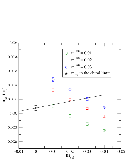
Figure 8: The residual mass determined from the WL-WL correlators. The solid line is a linear fit to the dynamical points with $m_{\rm val}=m_{l}^{\rm sea}$.

The quantitative description of the explicit chiral symmetry breaking for domain wall fermions is the residual mass, $m_{\rm res}$ Blum et al. (2004); Antonio et al. (2006a), which is determined from the ratio

$$R(t)=\frac{\langle\sum_{\bm{x}}J^{a}_{5q}(\bm{x},t)\pi^{a}(0)\rangle}{\langle\sum_{\bm{x}}J^{a}_{5}(\bm{x},t)\pi^{a}(0)\rangle}.$$ (7)

The definitions of $J^{a}_{5q}(\bm{x},t)$ and $J^{a}_{5}(\bm{x},t)$ for domain wall fermions can be found in Ref. Blum et al. (2004). We follow  Antonio et al. (2006a) and determine $m_{\rm res}$ at a given quark mass, denoted by $m_{\rm res}^{\prime}(m_{f})$, by fitting $R(t)$ to a constant over a time range where $R(t)$ shows a good plateau. The results from the WL-WL correlation functions are shown in Table 6.

While by definition $m_{\rm res}$ should be a constant, the operator we choose to determine it happens to depend on the quark mass, as shown in Figure 8. This quark mass dependence comes from the higher-dimension operators in the divergence of the axial current, which should be suppressed by powers of $a$ Antonio et al. (2006a); Lin (2006); Blum et al. (2002). We choose to deal with these lattice artifacts by extrapolating $m_{\rm res}^{\prime}(m_{f})$ to the zero quark mass limit in both the sea and valence sectors. Doing so gives

$$m_{\rm res}=0.00308(4).$$ (8)

This is about 1/3 of the lightest quark mass in our simulations, which may seem larger than ideal. Nevertheless, from a field theoretic point of view, to leading order the residual mass is just an additive renormalization to the input quark mass. Neglecting higher-order corrections, the chiral limit is defined at $m_{f}+m_{\rm res}=0$ or $m_{f}=-m_{\rm res}$, where $m_{f}$ is the input quark mass. This is the basis for the chiral extrapolations discussed in Section V. In this paper we do not attempt to discuss higher-order corrections to the residual mass, which should be small in our simulations.

Table 6: Residual mass obtained with the Coulomb gauge fixed wall source.

$m_{l}^{\rm sea}$	$m_{1}$	$m_{2}$	$t_{\rm min}-t_{\rm max}$	$\chi^{2}/dof$	$m_{\rm res}^{\prime}(m_{f})$
0.01	0.01	0.01	8-16	0.9(7)	0.003102(25)
0.01	0.02	0.02	8-16	1.0(7)	0.002962(23)
0.01	0.03	0.03	8-16	1.0(7)	0.002846(21)
0.01	0.04	0.04	8-16	0.9(7)	0.002752(19)
0.02	0.01	0.01	8-16	1.0(7)	0.003332(23)
0.02	0.02	0.02	8-16	0.9(7)	0.003197(20)
0.02	0.03	0.03	8-16	0.9(7)	0.003070(19)
0.02	0.04	0.04	8-16	0.9(7)	0.002961(18)
0.03	0.01	0.01	8-16	1.3(8)	0.003479(27)
0.03	0.02	0.02	8-16	1.5(9)	0.003337(24)
0.03	0.03	0.03	8-16	1.7(9)	0.003201(22)
0.03	0.04	0.04	8-16	1.9(10)	0.003085(20)

IV.4 Pseudoscalar Decay Constants

The decay constant $f_{P}$ for a charged pseudoscalar meson is defined by

$$-i\,f_{P}\,q_{\mu}e^{-iq\cdot x}={\langle\,0\,|\,{\cal A}_{\mu}(x)\,|\,\pi(\bm{q})\,\rangle},$$ (9)

where ${\cal A}_{\mu}(x)$ is the (partially) conserved axial vector current operator for domain wall fermions Blum et al. (2004), and $|\pi(\bm{q})\rangle$ is the state vector for a pseudoscalar meson with momentum $\bm{q}$. We normalize the state vector such that $\langle\pi(\bm{q})|\pi(\bm{q^{\prime}})\rangle=(2\pi)^{3}\,2\,E_{\bm{q}}\,\delta(\bm{q}-\bm{q^{\prime}})$. ${\cal A}_{\mu}$ is related to the local axial vector operator by ${\cal A}_{\mu}=Z_{A}A_{\mu}$ for physics at long distances. It is conventional to determine the matrix element of $\langle 0|{A}_{0}|\pi\rangle$ from the amplitude of the LL-LL correlation functions Antonio et al. (2006a); Blum et al. (2004), $A_{A_{0},A_{0}}^{LL}$. Here a double-cosh fit to the LL-LL and GG-GG correlation functions was performed to get a more reliable estimate of the amplitude of the LL-LL correlation functions. $f_{P}$ is obtained by

$$f^{(1)}_{P}=Z_{A}\sqrt{\frac{2A^{LL}_{A_{0},A_{0}}}{m_{P}}}.$$ (10)

A novel way of determining $f_{P}$ is from the WL-WL correlators. In contrast to the point-like sources, the normalization of the Coulomb gauge fixed wall source is not known analytically, and we need to compute the relative normalization of the source operator to the conserved current numerically. This can be done by employing the following ratio,

$$N_{W}=\frac{\sum_{\bm{x}}\langle{\cal A}_{0}(\bm{x},t)P^{W}(0)\rangle}{\sum_{\bm{x}}\langle A_{0}^{W}(\bm{x},t)P^{W}(0)\rangle},$$ (11)

where $P^{W}(0)$ is the Coulomb gauge fixed pseudoscalar source operator. The pseudoscalar decay constant can then be computed using the following formula:

$$f^{(2)}_{P}=\sqrt{\frac{2Z_{A}N_{W}A_{A_{0},A_{0}}^{WL}}{m_{P}}}.$$ (12)

This method has the advantage of giving smaller statistical errors compared to the conventional way of determining $f_{P}$ from the point-like sources. We note that here $N_{W}$ is merely a normalization factor for the two operators ${\cal A}_{0}(\bm{x},t)$ and $A_{0}^{W}(\bm{x},t)$ computed under the same condition. Unlike $Z_{A}$, which is a constant up to corrections of ${\cal O}(a^{2})$, the mass dependence of $N_{W}$ has physical significance and thus it is the value of $N_{W}$ evaluated at each valence quark mass that should be used in Eq.(12).

Table 7: $Z_{A}$ from WL-WL correlation functions for all three ensembles.

$m_{l}^{\rm sea}$	$m_{1}$	$m_{2}$	$t_{\rm min}-t_{\rm max}$	$\chi^{2}/dof$	$Z_{A}$
0.01	0.01	0.01	8-16	0.5(5)	0.71807(14)
0.01	0.02	0.02	8-16	0.7(6)	0.71930(11)
0.01	0.03	0.03	8-16	0.8(6)	0.72071(9)
0.01	0.04	0.04	8-16	0.9(7)	0.72222(8)
0.02	0.01	0.01	8-16	1.2(8)	0.71799(14)
0.02	0.02	0.02	8-16	1.0(7)	0.71925(10)
0.02	0.03	0.03	8-16	0.9(7)	0.72069(8)
0.02	0.04	0.04	8-16	0.8(7)	0.72221(7)
0.03	0.01	0.01	8-16	1.7(9)	0.71806(15)
0.03	0.02	0.02	8-16	2.0(10)	0.71931(11)
0.03	0.03	0.03	8-16	2.2(11)	0.72073(10)
0.03	0.04	0.04	8-16	2.2(10)	0.72226(9)

The value of $Z_{A}$ is determined using the method described in Antonio et al. (2006a) and Blum et al. (2004). We quote the results obtained from the WL-WL functions in Table 7. Results from other source-sink combinations are in good agreement with the shown values, although we do not display them in the paper. Taking the chiral limit removes an ${\cal O}(a^{2})$ lattice artifact and gives

$$Z_{A}=0.7162(2).$$ (13)

This is then used to extract $f_{P}$ from the axial vector correlators using either Eq.(10) or Eq.(12), the results of which are given in Tables 8 and 9, respectively. These two methods of extracting $f_{P}$ agree well, with the errors on $f_{P}^{(2)}$ being smaller than $f_{P}^{(1)}$ in most cases.

Table 8: Pseudoscalar decay constants as computed from the double-cosh fits to the LL-LL and GG-GG axial vector correlation functions for all three ensembles.

$m_{l}^{\rm sea}$	$m_{1}$	$m_{2}$	$f^{(1)}_{P}$
0.01	0.01	0.01	0.0893(13)
0.01	0.01	0.04	0.1007(12)
0.01	0.04	0.04	0.1116(10)
0.02	0.02	0.02	0.1003(8)
0.02	0.02	0.04	0.1070(6)
0.02	0.04	0.04	0.1133(7)
0.03	0.03	0.03	0.1094(13)
0.03	0.03	0.04	0.1111(12)
0.04	0.04	0.04	0.1143(12)

Table 9: Pseudoscalar decay constants as computed from the WL-WL axial vector correlation functions for all three ensembles.

$m_{l}^{\rm sea}$	$m_{1}$	$m_{2}$	$f^{(2)}_{P}$
0.01	0.01	0.01	0.0895(7)
0.01	0.02	0.02	0.0977(7)
0.01	0.03	0.03	0.1046(7)
0.01	0.04	0.04	0.1108(7)
0.02	0.01	0.01	0.0939(7)
0.02	0.02	0.02	0.1006(6)
0.02	0.03	0.03	0.1067(6)
0.02	0.04	0.04	0.1123(6)
0.03	0.01	0.01	0.0980(6)
0.03	0.02	0.02	0.1042(6)
0.03	0.03	0.03	0.1101(6)
0.03	0.04	0.04	0.1157(6)

V Observables in the Chiral Limit

Since we perform our simulations at quark masses that are heavier than the physical up and down quark masses, extrapolations are needed to obtain physical values for various quantities. Chiral perturbation theory is the correct effective theory to describe low-energy QCD and should be used to guide the extrapolations. However, the quark masses in our simulations are too heavy for next-to-leading-order (NLO) chiral perturbation theory to be consistent with our results Lin (2006). Although independent NLO fits for the pseudoscalar meson masses and decay constants are consistent with our data, our attempt to fit both simultaneously fails badly. This is to be expected since the pion masses at the light dynamical points in our simulations range from 400 MeV to 627 MeV. This mass scale is likely to be outside of the region where chiral perturbation theory is applicable. As will be demonstrated in the following, our data exhibits linear behavior in the range of quark masses in our simulations. Thus we resort to simple linear extrapolations to obtain physical results in the light quark mass limit. In many cases this coincides with the predictions of the leading-order chiral perturbation theory, but in fact the reason we are doing this is based purely on phenomenological observations, not from the underlying effective theory.

V.1 Determination of the Lattice Scale

We start out by setting the lattice scale for these simulations from the vector $\rho$ mass. Although at the lightest quark masses the vector meson mass in our simulations is slightly larger than the 2$m_{\pi}$ threshold, the requirement for non-zero relative momentum for the two pions prohibits the vector meson from decaying. We have chosen to do a partially quenched linear fit to the values of $m_{V}$ in Table 5, restricted to $m_{1}(m_{2})\leq 0.03$, with the following phenomenological form :

$$m_{V}=A\,(m_{l}^{\rm sea}+m_{\rm res})+B\,(m_{1}+m_{2}+2m_{\rm res})+C.$$ (14)

The values of the fit parameters are shown in Table 10. As an illustration, we show the fit curves through the $m_{l}^{\rm sea}=0.01$ data points and the unitary points in Figure 9. Setting $m_{1}=m_{2}=m_{l}^{\rm sea}=-m_{\rm res}$ gives the $\rho$ mass in the chiral limit, from which we determine the lattice scale to be

$$a^{-1}|_{\rho}=1.61(3)\,{\rm GeV}.$$ (15)

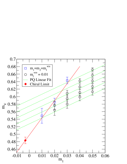
Figure 9: Linear extrapolations of the vector mass using Eq.(14). Here the circles are partially quenched data points from the $m_{l}^{\rm sea}=0.01$ ensemble, the squares are the unitary points with $m_{1}=m_{2}=m_{l}^{\rm sea}$ and the diamond is the value of $m_{V}$ in the chiral limit.

We also determined the lattice scale from the static quark potential using the Coulomb gauge method Bernard et al. (2000). The preliminary analysis of these ensembles was reported in Li (2006). More detailed analysis of this calculation is the subject of another paper in progress and will not be addressed here. We simply quote the updated value of the lattice scale determined using $r_{0}=0.5$ fm, which is

$$a^{-1}|_{r_{0}}=1.63(5)\,{\rm GeV}.$$ (16)

Our third choice for determining the lattice scale is the “method of lattice planes” Allton et al. (1997). In this approach the vector meson mass is plotted against the pseudoscalar meson mass squared and the interception of this data with the physical point $(m_{K}^{2},m_{K\ast})$ is found. Since the lattice data straddles the kaon data, a chiral interpolation rather than extrapolation is required in the valence quark sector. The results for the inverse lattice spacing for each of the sea quark masses is shown in Figure 10. Shown in this figure is a linear extrapolation in the sea quark mass to the chiral limit, $m_{l}^{\rm sea}=-m_{\rm res}$. In this limit, we obtain

$$a^{-1}|_{\rm lattice\ plane}=1.62(5)\ {\rm GeV}.$$ (17)

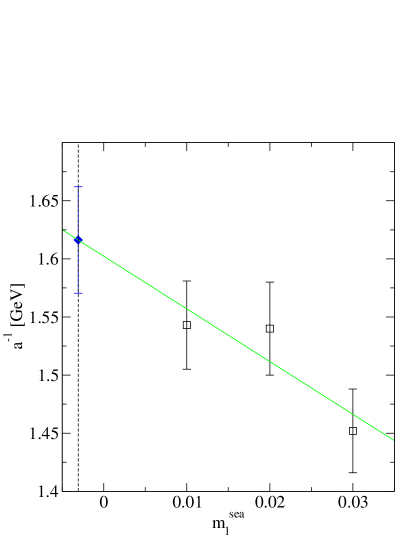
Figure 10: Linear extrapolation of $a^{-1}$ versus $m_{l}^{\rm sea}$ from the method of planes.

All these methods give consistent results for the lattice scale. However, each method has its own limitations. The physical $\rho$ meson is unstable and has the probability of decaying into two pions (though it is not the case in our simulations). The static quark potential suffers a small (few percent) uncertainty concerning the value of $r_{0}$. For the method of lattice planes, the extrapolation in the sea sector is purely phenomenological. Nevertheless, the three determinations of $a^{-1}$ agree well, so we take the average of these for our central value, and take as an error an average of the statistical errors. This gives

$$a^{-1}=1.62(4)\,{\rm GeV},$$ (18)

which will be used whenever a lattice scale is needed, and the errors will be propagated accordingly by quadrature.

V.2 Quark Masses and Decay Constants

A precise determination of the physical quark masses demands well-controlled chiral extrapolations in the light quark limit. As already mentioned, the relatively heavy quark masses in our simulations prevent us from using the next-to-leading order chiral perturbation theory to do the extrapolations. Again we restrict ourselves to linear extrapolation. We chose to fit only to the dynamical points where $m_{\rm val}=m_{l}^{\rm sea}$, using the following formula:

$$m_{P}^{2}=2B(m_{l}^{\rm sea}+m_{\rm res}).$$ (19)

The value of $B$ is given in Table 10. We then used the physical pion and kaon masses as inputs to determine the average light quark mass and the strange quark mass, as shown in Figure 11. The bare quark masses in lattice units are listed in the following:

$$\bar{m} = 0.00162(8)$$ (20)

$$m_{s} = 0.0390(21).$$ (21)

The above results have combined the bare input quark masses and the residual mass, and the quoted errors come from the errors on the pseudoscalar meson masses, the residual mass, and the lattice scale. Systematic uncertainties associated with the finite lattice spacing, chiral extrapolation and e-m splitting, etc. have not been investigated yet. We will employ the non-perturbative renormalization (NPR) technique Blum et al. (2002) to obtain the renormalized quark masses. The NPR analysis is still in progress.

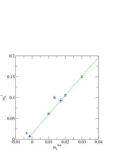
Figure 11: Linear extrapolation of the pseudoscalar meson mass through the light dynamical points. The crosses are the physical $\pi$ and $K$ points from which we obtain the values of $\bar{m}$ and $m_{s}$.

To obtain the physical results of $f_{\pi}$ and $f_{K}$, we fit the results of the pseudoscalar decay constants in Tables 9 and 8 to the following linear form separately:

$$f_{P}=f_{0}+L(\,m_{l}^{\rm sea}+m_{\rm res}).$$ (22)

We can see from Figure 12 that the data points are quite linear with our current statistics. The fitting parameters are also tabulated in Table 10. Using the quark masses and lattice scale determined in the above, we found that the physical values of $f_{\pi}$, $f_{K}$ and $f_{K}/f_{\pi}$ to be 126.9(45) MeV, 157.3(51) MeV and 1.240(31) respectively using $f_{P}^{(1)}$. Similar analysis using $f_{P}^{(2)}$ gives $f_{\pi}=126.7(36)$ MeV, $f_{K}=157.6(45)$ MeV and $f_{K}/f_{\pi}=1.244(20)$, which are consistent with the results from $f_{P}^{(1)}$. We take the averages of these two methods as our best estimates for these quantities, which are summarized in the following:

$$f_{\pi} = 127(4)\,\,{\rm MeV},$$ (23)

$$f_{K} = 157(5)\,\,{\rm MeV},$$ (24)

$$f_{K}/f_{\pi} = 1.24(2).$$ (25)

Our convention for the pseudoscalar decay constant is such that the experimental value of $f_{\pi}$ is about 131 MeV, $f_{K}$ about 160 MeV and $f_{K}/f_{\pi}$ about 1.22. Thus our results are in good agreement with the experiment.

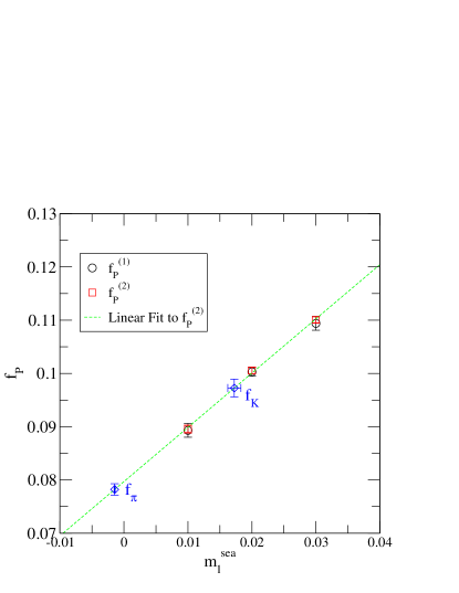
Figure 12: Linear extrapolation of the pseudoscalar meson decay constant through the light dynamical points. The diamonds are the values of $f_{\pi}$ and $f_{K}$ obtained from $f_{P}^{(2)}$.

Table 10: Linear fit parameters for various quantities.

$m_{V}$	$A=1.42(23)$	$B=1.58(16)$	$C=0.483(9)$
$m_{P}^{2}$		$B=2.285(24)$
$f_{P}^{(1)}$	$L=1.01(9)$	$f_{0}=0.0767(20)$
$f_{P}^{(2)}$	$L=1.02(5)$	$f_{0}=0.0765(11)$

We stress that these physical results are obtained in the context of simple linear extrapolations. Systematic uncertainties may arise from the presence of chiral logs. More sophisticated examination of the chiral behavior of various observables requires simulations at lighter quark masses, which will be further addressed in the near future. Nevertheless, such agreement is encouraging, and demonstrates that simulations with 2+1 flavors of domain wall fermions are promising.

VI Comparison of RHMC I and RHMC II

As discussed in Section III, there seem to be some long-range autocorrelations in these ensembles generated with 2+1 flavors of domain wall fermions. However, early simulations with two flavors of dynamical domain wall fermions did not have this problem Aoki et al. (2005). The biggest difference between those two-flavor simulations and this work lies in the way the following ratio is evaluated,

$$\frac{\det\left[D_{\rm DWF}^{\dagger}(M_{5},m_{s})D_{\rm DWF}(M_{5},m_{s})\right]}{\det\left[D_{\rm DWF}^{\dagger}(M_{5},1)D_{\rm DWF}(M_{5},1)\right]}.$$ (26)

In the two-flavor case, this ratio was evaluated using one pseudo-fermion field in the HMC evolution Aoki et al. (2005), which was found to reduce the stochastic noise substantially, and a larger step size could be used. At the beginning of these simulations this method had not yet been implemented in the RHMC algorithm, and two separate pseudo-fermion fields were needed to evaluate Eq. (26). Upon completion of the work reported in the previous sections, the new code was ready, and we were motivated to perform an extension of the $m_{l}^{\rm sea}=0.03$ ensemble using this new code to investigate any effects it might have on the ensemble properties. This variant of the RHMC algorithm, RHMC II, has been described in detail in Section II. From Table 1 we can see that the coarsest step size, $\delta\tau$, of RHMC II is almost twice as large as RHMC I, and fewer steps of intermediate and finest integration sizes are needed. We even obtained higher acceptance with these parameters. There is clearly at least a factor of two speedup by switching from RHMC I to RHMC II.

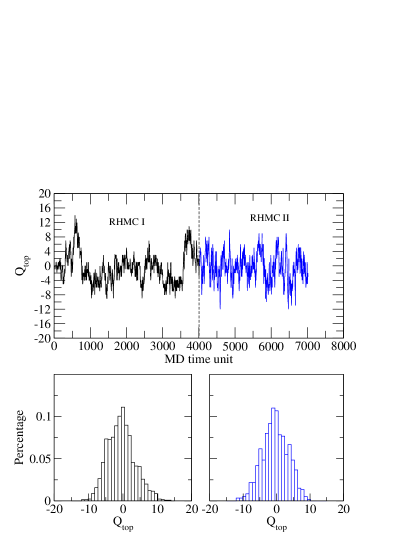
Figure 13: The comparison of the topological charge evolution and corresponding histogram measured from the two portions of the $m_{l}^{\rm sea}=0.03$ ensemble, in which different algorithms (RHMC I and RHMC II) were used to evaluate Eq.(1). The dashed line indicates where the algorithm was changed.

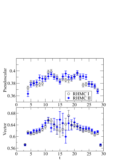
Figure 14: The comparison of the effective masses for the pseudoscalar and vector WL-WL correlation functions at the unitary point from the two portions of the $m_{l}^{\rm sea}=0.03$ ensemble (RHMC I and RHMC II).

Figure 13 shows the comparison of the evolution of the topological charge on the lattices generated using RHMC I and RHMC II. The tunneling of topological charge in RHMC II appears to be much better than RHMC I. The long-range autocorrelations present in RHMC I do not show up in RHMC II. This can be partly attributed to the use of a larger step size in the molecular dynamics evolution. Intuitively, a larger step size allows more efficient movement through, and the evolution is less likely to be trapped in a small region of, phase space. This consequently helps to move the topological charge from one sector to another. However, the histograms of the topological charge from these two segments of the ensemble are quite similar, indicating that RHMC I, while showing longer range autocorrelations, does give the same results as the improved version of the algorithm, RHMC II. We have also seen large fluctuations of the effective masses in Section IV. As a comparison, we show the effective masses for the pseudoscalar and vector WL-WL correlation functions, measured every 20 trajectories with $t_{\rm src}=0$ at the unitary point in Figure 14. While the vector effective mass remains noisy for RHMC II, there is noticeable improvement in the pseudoscalar effective mass, where a better plateau can be identified from $t=8$ to $t=24$.

We believe that RHMC II not only speeds up the gauge field generation by more than a factor of 2, but also helps to move through phase space more quickly and improve the quality of the ensembles we generate. The interplay of these two factors makes it a more favorable algorithm to use than RHMC I.

VII Conclusions

We have presented the results of light meson physics from lattice simulations with 2+1 flavors of dynamical domain wall fermions at a lattice spacing of about 0.12 fm in a (2 fm)³ volume. We used the improved RHMC algorithm to generate the gauge configurations, which turned out to be quite efficient in reducing the computing cost. Although there are some long-range autocorrelations in these ensembles, we have been able to obtain physical results with better than 5% statistical accuracy. The residual chiral symmetry breaking in these calculations is small compared to the earlier calculation with $L_{s}=8$ Antonio et al. (2006a), which gives us better control over chiral symmetry breaking effects. We have shown results for the bare physical quark masses and decay constants, the latter in good agreement with their experimental values. We have also shown that a newly improved variant of the RHMC algorithm, RHMC II, not only speeds up the gauge field generation by more than a factor of 2, but also moves through phase space more efficiently.

There are of course some systematic uncertainties that we have yet to control. One is the failure of even our lightest quark mass data to permit chiral extrapolations which follow the form predicted by chiral perturbation theory. We did not attempt to perform simulations at even lighter quark masses on these lattices, because the volume for such simulations may be too small, which could result in sizable finite volume effects. To pursue this issue further, the RBC and UKQCD collaborations are performing 2+1 flavor simulations on a $24^{3}\times 64$ volume, or about (3 fm)³ in physical units, at about the same lattice spacing. This larger volume allows calculations with lighter quark masses, from which we hope to investigate the light quark limit in the context of chiral perturbation theory. Comparing the physical results in two different volumes will also enable us to quantitatively study finite volume effects. This will be especially important for baryon physics. Secondly, more than one lattice spacing is needed to investigate the scaling behavior for domain wall fermions and the Iwasaki gauge action, and the continuum limit should be taken to remove lattice artifacts. We will address this question in upcoming simulations in a (3 fm)³ volume at a weaker coupling.

With good control over chiral symmetry and an exact and efficient algorithm, we are vigorously pursuing 2+1 flavor domain wall QCD. The theoretical promise of this approach is now producing numerical results for the physically interesting 2+1 flavor case.

Appendix A Tables of Meson Masses

Table 11: Pseudoscalar meson masses from GL-GL correlation functions as determined from the pseudoscalar channel.

$m_{l}^{\rm sea}$	$m_{1}$	$m_{2}$	$t_{\rm min}-t_{\rm max}$	$\chi^{2}$/dof	$m_{P}$
0.01	0.01	0.01	8-16	0.6(6)	0.2460(10)
0.01	0.01	0.04	8-16	0.8(6)	0.3545(8)
0.01	0.04	0.04	8-16	1.1(7)	0.4382(7)
0.02	0.02	0.02	8-16	0.9(7)	0.3247(8)
0.02	0.02	0.04	8-16	0.9(7)	0.3868(8)
0.02	0.04	0.04	8-16	0.9(7)	0.4410(7)
0.03	0.03	0.03	8-16	3.8(15)	0.3907(15)
0.03	0.03	0.04	8-16	3.6(14)	0.4184(14)
0.03	0.04	0.04	8-16	3.5(14)	0.4446(13)

Table 12: Pseudoscalar meson masses from GL-GL correlation functions as determined from the axial vector channel.

$m_{l}^{\rm sea}$	$m_{1}$	$m_{2}$	$t_{\rm min}-t_{\rm max}$	$\chi^{2}$/dof	$m_{P}$
0.01	0.01	0.01	8-16	2.4(10)	0.2467(15)
0.01	0.01	0.04	8-16	1.9(8)	0.3547(14)
0.01	0.04	0.04	8-16	2.0(9)	0.4379(10)
0.02	0.02	0.02	9-16	2.1(10)	0.3254(12)
0.02	0.02	0.04	9-16	1.8(9)	0.3877(10)
0.02	0.04	0.04	9-16	1.7(9)	0.4413(10)
0.03	0.03	0.03	7-16	3.2(11)	0.3881(16)
0.03	0.03	0.04	7-16	2.8(10)	0.4170(16)
0.03	0.04	0.04	7-16	1.7(9)	0.4425(13)

Table 13: Vector meson masses from GL-GL correlation functions for all three ensembles.

$m_{l}^{\rm sea}$	$m_{1}$	$m_{2}$	$t_{\rm min}-t_{\rm max}$	$\chi^{2}/dof$	$m_{V}$
0.01	0.01	0.01	10-16	0.7(7)	0.558(12)
0.01	0.01	0.04	10-16	0.6(6)	0.6016(45)
0.01	0.04	0.04	10-16	0.7(7)	0.6443(23)
0.02	0.02	0.02	10-16	1.4(10)	0.5914(69)
0.02	0.02	0.04	10-16	0.7(8)	0.6217(47)
0.02	0.04	0.04	10-16	0.4(6)	0.6524(35)
0.03	0.03	0.03	10-16	0.7(8)	0.6519(75)
0.03	0.03	0.04	10-16	0.7(7)	0.6643(63)
0.03	0.04	0.04	10-16	0.6(7)	0.6771(54)

Table 14: Pseudoscalar meson masses as determined from the WL-WL pseudoscalar correlation functions.

$m_{l}^{\rm sea}$	$m_{1}$	$m_{2}$	$t_{\rm min}-t_{\rm max}$	$\chi^{2}$/dof	$m_{P}$
0.01	0.01	0.01	9-16	1.1(9)	0.2474(16)
0.01	0.02	0.02	9-16	1.3(9)	0.3223(14)
0.01	0.03	0.03	9-16	1.4(10)	0.3836(12)
0.01	0.04	0.04	9-16	1.6(10)	0.4373(11)
0.02	0.01	0.01	9-16	1.1(8)	0.2458(15)
0.02	0.02	0.02	9-16	1.3(9)	0.3212(12)
0.02	0.03	0.03	9-16	1.6(10)	0.3832(11)
0.02	0.04	0.04	9-16	1.9(11)	0.4378(10)
0.03	0.01	0.01	9-16	3.5(15)	0.2551(19)
0.03	0.02	0.02	9-16	3.6(15)	0.3282(16)
0.03	0.03	0.03	9-16	3.5(15)	0.3891(15)
0.03	0.04	0.04	9-16	3.4(15)	0.4429(13)

Table 15: Pseudoscalar meson masses from WL-WL correlation functions as determined from the axial vector channel.

$m_{l}^{\rm sea}$	$m_{1}$	$m_{2}$	$t_{\rm min}-t_{\rm max}$	$\chi^{2}$/dof	$m_{P}$
0.01	0.01	0.01	8-16	0.8(7)	0.2466(16)
0.01	0.02	0.02	8-16	0.6(6)	0.3215(14)
0.01	0.03	0.03	8-16	0.8(7)	0.3828(13)
0.01	0.04	0.04	8-16	1.2(8)	0.4365(12)
0.02	0.01	0.01	8-16	1.4(9)	0.2479(13)
0.02	0.02	0.02	8-16	1.6(10)	0.3226(11)
0.02	0.03	0.03	8-16	1.7(10)	0.3842(10)
0.02	0.04	0.04	8-16	1.9(10)	0.4385(9)
0.03	0.01	0.01	8-16	2.2(11)	0.2526(14)
0.03	0.02	0.02	8-16	3.0(13)	0.3268(14)
0.03	0.03	0.03	8-16	2.9(13)	0.3884(13)
0.03	0.04	0.04	8-16	2.8(13)	0.4427(11)

Table 16: Vector meson masses from WL-WL correlation functions for all three ensembles.

$m_{l}^{\rm sea}$	$m_{1}$	$m_{2}$	$t_{\rm min}-t_{\rm max}$	$\chi^{2}/dof$	$m_{V}$
0.01	0.01	0.01	9-16	1.2(9)	0.542(11)
0.01	0.02	0.02	9-16	1.9(11)	0.5742(58)
0.01	0.03	0.03	9-16	1.9(11)	0.6078(38)
0.01	0.04	0.04	9-16	1.6(10)	0.6402(29)
0.02	0.01	0.01	6-16	0.8(6)	0.5533(44)
0.02	0.02	0.02	6-16	0.8(6)	0.5845(30)
0.02	0.03	0.03	6-16	0.9(6)	0.6162(23)
0.02	0.04	0.04	6-16	1.1(7)	0.6475(19)
0.03	0.01	0.01	10-16	0.9(8)	0.621(16)
0.03	0.02	0.02	10-16	0.8(8)	0.6253(82)
0.03	0.03	0.03	10-16	1.0(9)	0.6464(55)
0.03	0.04	0.04	10-16	1.4(11)	0.6718(42)

Table 17: Pseudoscalar meson masses from WL-WL correlation functions with P+A boundary conditions as determined from the pseudoscalar channel.

$m_{l}^{\rm sea}$	$m_{1}$	$m_{2}$	$t_{\rm min}-t_{\rm max}$	$m_{P}$
0.01	0.01	0.01	10-22	0.2509(22)
0.01	0.02	0.01	10-22	0.2913(21)
0.01	0.02	0.02	10-22	0.3262(19)
0.01	0.03	0.01	10-22	0.3270(20)
0.01	0.03	0.02	10-22	0.3583(19)
0.01	0.03	0.03	10-22	0.3877(18)
0.01	0.04	0.01	10-22	0.3594(20)
0.01	0.04	0.02	10-22	0.3881(18)
0.01	0.04	0.03	10-22	0.4155(18)
0.01	0.04	0.04	10-22	0.4416(17)
0.01	0.05	0.01	10-22	0.3894(20)
0.01	0.05	0.02	10-22	0.4161(18)
0.01	0.05	0.03	10-22	0.4418(18)
0.01	0.05	0.04	10-22	0.4666(17)
0.01	0.05	0.05	10-22	0.4906(17)
0.02	0.01	0.01	10-22	0.2527(20)
0.02	0.02	0.01	10-22	0.2910(19)
0.02	0.02	0.02	10-22	0.3251(18)
0.02	0.03	0.01	10-22	0.3253(19)
0.02	0.03	0.02	10-22	0.3564(17)
0.02	0.03	0.03	10-22	0.3855(17)
0.02	0.04	0.01	10-22	0.3567(19)
0.02	0.04	0.02	10-22	0.3856(17)
0.02	0.04	0.03	10-22	0.4129(16)
0.02	0.04	0.04	10-22	0.4390(15)
0.02	0.05	0.01	10-22	0.3859(19)
0.02	0.05	0.02	10-22	0.4131(17)
0.02	0.05	0.03	10-22	0.4390(16)
0.02	0.05	0.04	10-22	0.4639(15)
0.02	0.05	0.05	10-22	0.4878(15)
0.03	0.01	0.01	10-22	0.2496(21)
0.03	0.02	0.01	10-22	0.2885(19)
0.03	0.02	0.02	10-22	0.3227(19)
0.03	0.03	0.01	10-22	0.3235(19)
0.03	0.03	0.02	10-22	0.3544(18)
0.03	0.03	0.03	10-22	0.3837(18)
0.03	0.04	0.01	10-22	0.3556(19)
0.03	0.04	0.02	10-22	0.3841(18)
0.03	0.04	0.03	10-22	0.4116(17)
0.03	0.04	0.04	10-22	0.4379(17)
0.03	0.05	0.01	10-22	0.3854(19)
0.03	0.05	0.02	10-22	0.4120(18)
0.03	0.05	0.03	10-22	0.4380(17)
0.03	0.05	0.04	10-22	0.4631(17)
0.03	0.05	0.05	10-22	0.4873(16)

Table 18: Pseudoscalar meson masses from WL-WL correlation functions with P+A boundary conditions as determined from the axial vector channel.

$m_{l}^{\rm sea}$	$m_{1}$	$m_{2}$	$t_{\rm min}-t_{\rm max}$	$m_{P}$
0.01	0.01	0.01	10-22	0.2473(23)
0.01	0.02	0.01	10-22	0.2878(21)
0.01	0.02	0.02	10-22	0.3231(19)
0.01	0.03	0.01	10-22	0.3236(20)
0.01	0.03	0.02	10-22	0.3552(18)
0.01	0.03	0.03	10-22	0.3847(17)
0.01	0.04	0.01	10-22	0.3560(20)
0.01	0.04	0.02	10-22	0.3850(17)
0.01	0.04	0.03	10-22	0.4124(16)
0.01	0.04	0.04	10-22	0.4386(15)
0.01	0.05	0.01	10-22	0.3860(19)
0.01	0.05	0.02	10-22	0.4130(17)
0.01	0.05	0.03	10-22	0.4388(16)
0.01	0.05	0.04	10-22	0.4637(15)
0.01	0.05	0.05	10-22	0.4877(15)
0.02	0.01	0.01	10-22	0.2535(22)
0.02	0.02	0.01	10-22	0.2938(20)
0.02	0.02	0.02	10-22	0.3287(19)
0.02	0.03	0.01	10-22	0.3292(20)
0.02	0.03	0.02	10-22	0.3605(18)
0.02	0.03	0.03	10-22	0.3897(17)
0.02	0.04	0.01	10-22	0.3612(19)
0.02	0.04	0.02	10-22	0.3899(17)
0.02	0.04	0.03	10-22	0.4171(16)
0.02	0.04	0.04	10-22	0.4430(16)
0.02	0.05	0.01	10-22	0.3907(19)
0.02	0.05	0.02	10-22	0.4175(17)
0.02	0.05	0.03	10-22	0.4431(16)
0.02	0.05	0.04	10-22	0.4677(15)
0.02	0.05	0.05	10-22	0.4914(15)
0.03	0.01	0.01	10-22	0.2486(23)
0.03	0.02	0.01	10-22	0.2886(22)
0.03	0.02	0.02	10-22	0.3235(21)
0.03	0.03	0.01	10-22	0.3242(22)
0.03	0.03	0.02	10-22	0.3555(20)
0.03	0.03	0.03	10-22	0.3849(19)
0.03	0.04	0.01	10-22	0.3565(22)
0.03	0.04	0.02	10-22	0.3852(20)
0.03	0.04	0.03	10-22	0.4126(19)
0.03	0.04	0.04	10-22	0.4388(18)
0.03	0.05	0.01	10-22	0.3863(22)
0.03	0.05	0.02	10-22	0.4131(20)
0.03	0.05	0.03	10-22	0.4389(19)
0.03	0.05	0.04	10-22	0.4637(18)
0.03	0.05	0.05	10-22	0.4877(17)

Table 19: Vector meson masses from WL-WL correlation functions with P+A boundary conditions for all three ensembles.

$m_{l}^{\rm sea}$	$m_{1}$	$m_{2}$	$t_{\rm min}-t_{\rm max}$	$m_{V}$
0.01	0.01	0.01	6-14	0.546(13)
0.01	0.02	0.01	6-14	0.563(9)
0.01	0.02	0.02	6-14	0.579(7)
0.01	0.03	0.01	6-14	0.580(7)
0.01	0.03	0.02	6-14	0.595(6)
0.01	0.03	0.03	6-14	0.610(5)
0.01	0.04	0.01	6-14	0.597(6)
0.01	0.04	0.02	6-14	0.611(5)
0.01	0.04	0.03	6-14	0.626(5)
0.01	0.04	0.04	6-14	0.641(4)
0.01	0.05	0.01	6-14	0.613(6)
0.01	0.05	0.02	6-14	0.627(5)
0.01	0.05	0.03	6-14	0.642(4)
0.01	0.05	0.04	6-14	0.657(4)
0.01	0.05	0.05	6-14	0.672(3)
0.02	0.01	0.01	6-14	0.538(13)
0.02	0.02	0.01	6-14	0.560(10)
0.02	0.02	0.02	6-14	0.579(7)
0.02	0.03	0.01	6-14	0.579(8)
0.02	0.03	0.02	6-14	0.597(6)
0.02	0.03	0.03	6-14	0.614(5)
0.02	0.04	0.01	6-14	0.597(7)
0.02	0.04	0.02	6-14	0.614(5)
0.02	0.04	0.03	6-14	0.631(5)
0.02	0.04	0.04	6-14	0.647(4)
0.02	0.05	0.01	6-14	0.614(6)
0.02	0.05	0.02	6-14	0.631(5)
0.02	0.05	0.03	6-14	0.647(4)
0.02	0.05	0.04	6-14	0.663(4)
0.02	0.05	0.05	6-14	0.679(4)
0.03	0.01	0.01	6-14	0.577(15)
0.03	0.02	0.01	6-14	0.589(11)
0.03	0.02	0.02	6-14	0.601(8)
0.03	0.03	0.01	6-14	0.603(9)
0.03	0.03	0.02	6-14	0.616(7)
0.03	0.03	0.03	6-14	0.630(6)
0.03	0.04	0.01	6-14	0.618(7)
0.03	0.04	0.02	6-14	0.631(6)
0.03	0.04	0.03	6-14	0.645(5)
0.03	0.04	0.04	6-14	0.660(4)
0.03	0.05	0.01	6-14	0.633(6)
0.03	0.05	0.02	6-14	0.646(5)
0.03	0.05	0.03	6-14	0.660(5)
0.03	0.05	0.04	6-14	0.675(4)
0.03	0.05	0.05	6-14	0.690(4)

References

- Kaplan (1992) D. B. Kaplan, Phys. Lett. B288, 342 (1992), eprint hep-lat/9206013.
- Shamir (1993) Y. Shamir, Nucl. Phys. B406, 90 (1993), eprint hep-lat/9303005.
- Furman and Shamir (1995) V. Furman and Y. Shamir, Nucl. Phys. B439, 54 (1995), eprint hep-lat/9405004.
- Blum et al. (2003) T. Blum et al. (RBC), Phys. Rev. D68, 114506 (2003), eprint hep-lat/0110075.
- Noaki et al. (2003) J. I. Noaki et al. (CP-PACS), Phys. Rev. D68, 014501 (2003), eprint hep-lat/0108013.
- Golterman and Shamir (2005) M. Golterman and Y. Shamir, Phys. Rev. D71, 034502 (2005), eprint hep-lat/0411007.
- Christ (2005) N. Christ (RBC and UKQCD), Proc. Sci. LAT2005, 345 (2005).
- Blum et al. (2004) T. Blum et al., Phys. Rev. D69, 074502 (2004), eprint hep-lat/0007038.
- Blum et al. (2002) T. Blum et al., Phys. Rev. D66, 014504 (2002), eprint hep-lat/0102005.
- Clark (2006) M. A. Clark (2006), eprint hep-lat/0610048.
- Antonio et al. (2006a) D. J. Antonio et al. (2006a), eprint hep-lat/0612005.
- Clark and Kennedy (2004) M. A. Clark and A. D. Kennedy, Nucl. Phys. Proc. Suppl. 129, 850 (2004), eprint hep-lat/0309084.
- Clark et al. (2005) M. A. Clark, A. D. Kennedy, and Z. Sroczynski, Nucl. Phys. Proc. Suppl. 140, 835 (2005), eprint hep-lat/0409133.
- Clark et al. (2006) M. A. Clark, P. de Forcrand, and A. D. Kennedy, PoS LAT2005, 115 (2006), eprint hep-lat/0510004.
- Antonio et al. (2006b) D. Antonio et al. (RBC and UKQCD), PoS LAT2006, 188 (2006b).
- Kennedy et al. (1999) A. D. Kennedy, I. Horvath, and S. Sint, Nucl. Phys. Proc. Suppl. 73, 834 (1999), eprint hep-lat/9809092.
- Clark and Kennedy (2006) M. A. Clark and A. D. Kennedy (2006), eprint hep-lat/0608015.
- Sexton and Weingarten (1992) J. C. Sexton and D. H. Weingarten, Nucl. Phys. B380, 665 (1992).
- Omelyan and Folk (2003) I. M. Omelyan, I. P. Mryglod and R. Folk, Comp. Phys. Comm. 151, 272 (2003).
- Takaishi and de Forcrand (2006) T. Takaishi and P. de Forcrand, Phys. Rev. E73, 036706 (2006), eprint hep-lat/0505020.
- Urbach et al. (2006) C. Urbach, K. Jansen, A. Shindler, and U. Wenger, Comput. Phys. Commun. 174, 87 (2006), eprint hep-lat/0506011.
- Aoki et al. (2005) Y. Aoki et al., Phys. Rev. D72, 114505 (2005), eprint hep-lat/0411006.
- Hasenbusch and Jansen (2003) M. Hasenbusch and K. Jansen, Nucl. Phys. B659, 299 (2003), eprint hep-lat/0211042.
- Allton et al. (1993) C. R. Allton et al. (UKQCD), Phys. Rev. D47, 5128 (1993), eprint hep-lat/9303009.
- Lin (2006) M. Lin (RBC), PoS LAT2006, 185 (2006), eprint hep-lat/0610052.
- Bernard et al. (2000) C. W. Bernard et al., Phys. Rev. D62, 034503 (2000), eprint hep-lat/0002028.
- Li (2006) M. Li, PoS LAT2006, 183 (2006), eprint hep-lat/0610106.
- Allton et al. (1997) C. R. Allton, V. Gimenez, L. Giusti, and F. Rapuano, Nucl. Phys. B489, 427 (1997), eprint hep-lat/9611021.