Deconfining Phase Transition on Lattices with Boundaries at Low Temperature

Abstract

In lattice gauge theory (LGT) equilibrium simulations of QCD are usually performed with periodic boundary conditions (BCs). In contrast to that deconfined regions created in heavy ion collisions are bordered by the confined phase. Here we discuss BCs in LGT, which model a cold exterior of the lattice volume. Subsequently we perform Monte Carlo (MC) simulations of pure SU(3) LGT with a thus inspired simple change of BCs using volumes of a size comparable to those typically encountered in the BNL relativistic heavy ion collider (RHIC) experiment. Corrections to the usual LGT results survive in the finite volume continuum limit and we estimate them as function of the volume size. In magnitude they are found comparable to those of including quarks. As observables we use a pseudocritical temperature, which rises opposite to the effect of quarks, and the width of the transition, which broadens similar to the effect of quarks.

I Introduction

At a sufficiently high temperature QCD is known to undergo a phase transition from our everyday phase, where quarks and gluons are confined, to a deconfined quark-gluon plasma. Since the early days of lattice gauge theory simulations of this transition have been a subject of the field Tc-old , see Tc-now for reviews. Naturally, such simulations focused on boundary conditions (BCs), which are favorable for reaching the infinite volume quantum quantum continuum limit quickly. On lattices of size $N_{\tau}\,N_{s}^{3}$ these are periodic BCs in the spatial volume $V=(a\,N_{s})^{3}$, where $a$ is the lattice spacing. For a textbook, see, e.g., Ref. Rothe .

The physical temperature of the system on a $N_{\tau}\,N_{s}^{3}$ lattice, $N_{\tau}<N_{s}$, is given by

$$T=\frac{1}{a\,N_{\tau}}=\frac{1}{L_{\tau}}$$ (1)

where $a$ is the lattice spacing. In this paper we set the physical scale by note ,

$$T^{c}=174\ {\rm MeV}$$ (2)

for the deconfinement temperature, which is approximately the average from QCD estimates with two light flavor quarks Tc-now in the infinite volume extrapolation. The relation (1) implies for the temporal extension of the system

$$L_{\tau}=a\,N_{\tau}=1.13\ {\rm fermi}\ .$$ (3)

For the deconfinement phase created in a RHIC the infinite volume limit $N_{s}/N_{\tau}\to\infty$ for fixed $N_{\tau}$ and subsequently $N_{\tau}\to\infty$ ($L_{\tau}=a\,N_{\tau}$ finite) does not apply. Instead we have to take the continuum limit as

$$N_{s}/N_{\tau}={\rm finite}\,,~{}~{}N_{\tau}\to\infty\,,~{}~{}L_{\tau}~{}~{}{\rm finite}\,,$$ (4)

and periodic BCs are incorrect because the outside is in the confined phase at low temperature. Details are discussed in the next section.

In collisions at the BNL RHIC RHIC one expects to create an ensemble of differently shaped and sized volumes, which contain the deconfined quark-gluon plasma. The largest volumes are those encountered in central collisions. A rough estimate of their size is

$$\pi\times(0.6\times{\rm Au\ radius})^{2}\times c\times({\rm expansion\ time})$$

$$=(55\ {\rm fermi}^{2})\times({\rm a\ few\ fermi})$$ (5)

where $c$ is the speed of light. To imitate this geometry, one may want to model spatial volumes of cylindrical and other geometries. In our exploratory study we do not try to imitate a realistic ensemble of deconfined volumes, but are content to estimate the magnitude of corrections one may expect. So we stay with $N_{s}^{3}$ volumes and focus on results in the continuum limit for

$$L_{s}=aN_{s}=(5-10)\ {\rm fermi}\ .$$ (6)

Finite volume corrections to the infinite volume continuum limit are expected to be relevant as long as the volume is not large compared to a typical hadronic correlation length, which is about one fermi. For relatively small volumes an appropriate modeling of the BCs is necessary.

In the next section we introduce BCs, which reflect a (very) low temperature outside of the deconfined region. Two constructions, the “disorder wall” and the “confinement wall” are carried out and shown to exhibit the usual asymptotic scaling properties in the finite volume continuum limit. While the confined wall is physically more accurate, the disorder wall can be easily implemented in MC calculations. For the latter MC calculations of pure SU(3) LGT are performed in section III and evidence for scaling is already found for systems sizes which can be simulated on PC clusters. Summary and conclusion are given in section IV.

II Boundary Conditions

Statistical properties of a quantum system with Hamiltonian $H$ in a continuum volume $V$, which is in equilibrium with a heatbath at physical temperature $T$, are determined by the partition function Rothe

$$Z(T,V)={\rm Tr}e^{-H/T}=\sum_{\phi}\langle\phi|e^{-H/T}|\phi\rangle,$$ (7)

where the sum extends over all possible states $|\phi\rangle$ of the system and the Boltzmann constant is set to one. Imposing periodic boundary conditions in Euclidean time $\tau$ and bounds of integration from $0$ to $1/T$, one can rewrite the partition function (7) in the path integral representation:

$$Z(T,V)=\int D\phi\exp\left\{-\int_{0}^{1/T}d\tau L_{E}(\phi,\dot{\phi})\right\}.$$ (8)

Nothing in this formulation requires to carry out the infinite volume limit. In the contrary, if one deals with rather small volumes for which fluctuations of the mean values are not negligible, the idea to consider $V\to\infty$ instead of $V$ appears to be rather obscure.

An obvious problem of applying equilibrium thermodynamics to deconfined volumes at RHIC is that there is no heatbath in sight with which the system could be in equilibrium. However, arguments have been made in the literature that after the rapid heating quench, when the deconfined volume is at about its maximum size, a (pseudo) equilibrium state is reached for a transitional period, which is reasonably long on the scale of the relaxation times involved. These arguments are not beyond doubts (some are raised in one of our own papers Ba06 ), but they are not a topic of our present work. Here our assumption is that there is some truth to the belief that the bulk properties can be described by equilibrated finite temperature QCD.

In MC simulation the updating process provides the heatbath and finite volumes can be equilibrated with all kind of BCs imposed, although in practice most simulations have used periodic BCs. For simplicity and to be definite we restrict our discussion to pure SU(3) LGT. Generalization of the arguments of this section to full QCD appears to be straightforward. We use the Wilson action given by

$$S(\{U\})=\frac{\beta^{g}}{3}\sum_{\Box}{\rm Re}\,{\rm Tr}\left(U_{\Box}\right)\,,$$ (9)

$U_{\Box}=U_{i_{1}j_{1}}U_{j_{1}i_{2}}U_{i_{2}j_{2}}U_{j_{2}i_{1}}$, where the sum is over all plaquettes of a 4D simple hypercubic lattice, $i_{1},\,j_{1},\,i_{2}$ and $j_{2}$ label the sites circulating about the plaquette and $U_{ji}$ is the $SU(3)$ matrix associated with the link $\langle ij\rangle$. The reversed link is associated with the inverse matrix, and $\beta^{g}$ is related to the bare coupling constant by $\beta^{g}=6/g^{2}$. The theory is defined by the expectation values of its operators with respect to the Euclidean path integral

$$Z=\int\prod_{\langle ij\rangle}dU_{ij}\,e^{S\left(\{U\}\right)}\,,$$ (10)

where the integrations are over the invariant group measure, which was for compact groups like SU(3) introduced by Hurwitz Hu (Haar Ha generalized it later).

Numerical evidence suggests that for $N_{\tau}$ fixed and $N_{s}\to\infty$ SU(3) lattice gauge theory exhibits a deconfining phase transition (sub- or superscript $t$ stand for transition) at some coupling $\beta^{g}_{t}(N_{\tau})=6/g^{2}_{t}(N_{\tau})$, which is weakly first order firstorder . The scaling behavior of the deconfining temperature is

$$T^{c}=c_{T}\,\Lambda_{L}$$ (11)

where $c_{T}$ is a constant and we use the lambda lattice scale

$$a\,\Lambda_{L}=f_{\lambda}(\beta^{g})=\lambda(g^{2})\,\left(b_{0}\,g^{2}\right)^{-b_{1}/(2b_{0}^{2})}\,e^{-1/(2b_{0}\,g^{2})}\,,$$ (12)

where $a$ is the lattice spacing. The coefficients $b_{0}$ and $b_{1}$ are perturbatively determined by the renormalization group equation and independent of the renormalization prescription AF ,

$$b_{0}=\frac{11}{3}\frac{3}{16\pi^{2}}~{}~{}{\rm and}~{}~{}b_{1}=\frac{34}{3}\left(\frac{3}{16\pi^{2}}\right)^{2}\,.$$ (13)

For perturbative and non-perturbative corrections we adopt the analysis of Bo96 in the parameterization of Ba06a :

$$\lambda(g^{2})\ =\ 1+a_{1}\,e^{-a_{2}/g^{2}}+a_{3}\,g^{2}+a_{4}\,g^{4}$$ (14)

with $a_{1}=71553750$, $a_{2}=19.48099$, $a_{3}=-0.03772473$, and $a_{4}=0.5089052$.

We want to model an equilibrium situation surrounded by cold boundaries at $300\,$K. The effects are expected to penetrate at least a few correlation lengths into the volume. Note that this is the correlation length set by hadronic interaction, which can be defined by an appropriate inverse mass. On the lattice $\xi/a$ governs the continuum limit. This should not be confused with correlations due to the phase transition. As the lattice regularization allows to construct finite volume continuum limits as well as the infinite volume continuum limit, the question is: Which construction has the best chances to capture the physics realistically for a quark-gluon plasma in a small volume as typically created at RHIC?

Let us first exemplify that LGT thermodynamics allows not only to approach the infinite volume continuum limit, but also finite volume continuum limits. For instance, we can define the thermodynamics on a torus which has the volume of, say, $(10\,{\rm fermi})^{3}$. To achieve a continuum limit, we have to send the lattice spacing $a\to 0$ in units of the physical scale. This is governed by the renormalization group equation and requires infinitely many lattice points $N_{s}=L_{s}/a\to\infty$, while the physical volume of the lattice stays finite by arranging $L_{s}/{\rm fermi}=c_{1}$, where $c_{1}$ is a constant, e.g., $c_{1}=10$. The temperature of such a system is regulated by choosing $L_{\tau}/L_{s}=c_{2}$, where $c_{2}$ is a second constant. For describing deconfined volumes at RHIC the thus defined toroidal mini-universe is even less suitable than the conventionally used infinite volume limit, because correlations are artificially propagated through the periodic BCs. We present now two constructions of BCs, which reflect cold exterior volumes. The second is physically more realistic, but numerically more difficult to implement.

II.1 Disorder wall

Imagine an almost infinite space volume $V=L_{s}^{3}$, which may have periodic BCs, and a smaller (very large, but small compared to $V$) sub-volume $V_{0}=L_{s,0}^{3}$. The complement to $V_{0}$ in $V$ will be called $V_{1}$. The number of temporal lattice links $N_{\tau}$ is the same for both volumes. We want to find $\beta^{g}$ values and lattice dimensions so that scaling holds, while $V_{0}$ is at a temperature of $T_{0}=174\,{\rm MeV}$ and $V_{1}$ at $T_{1}=300\,{\rm K}$. We set the coupling $\beta^{g}$ to $\beta^{g}_{0}$ for plaquettes in $V_{0}$ and to $\beta^{g}_{1}$ for plaquettes in $V_{1}$. For that purpose any plaquette touching a site in $V_{1}$ is considered to be in $V_{1}$. Let us take $\beta^{g}_{1}=5.7$, which is at the beginning of the SU(3) scaling region. We have $174\,{\rm MeV}=2.02\times 10^{12}\,{\rm K}$ and, therefore,

$$\frac{T_{0}}{T_{1}}=\frac{2.02\times 10^{12}}{300}=\frac{a_{1}}{a_{0}}=\frac{f_{\lambda}(\beta^{g}_{1})}{f_{\lambda}(\beta^{g}_{0})}$$ (15)

where $a_{i}$ is the lattice spacing in $V_{i},\,i=0,1$. Using (12) the scaling equation

$$300\,f_{\lambda}(\beta^{g}_{1})=2.02\times 10^{12}\,f_{\lambda}(\beta^{g}_{0})$$ (16)

yields $\beta^{g}_{0}=24.496$. $T_{c}$ estimates from MC calculations of the literature extrapolate then to $L_{\tau}\geq 2.74\times 10^{10}\,a$ for the temporal lattice extension needed for a deconfined phase at $\beta^{g}_{0}=24.5$. This illustrates the orders of magnitude involved.

So, in practice we can only have $\beta^{g}_{0}$, but not $\beta^{g}_{1}$ in the scaling region, say $\beta^{g}_{0}=6$. There is still a reasonable choice for $\beta^{g}_{1}$. The scaling argument (15) shows that in lattice units a correlation length $\xi$, say one fermi, is at $\beta^{g}_{0}$ much larger than at $\beta^{g}_{1}$:

$$\frac{(\xi/a_{0})}{(\xi/a_{1})}=\frac{a_{1}}{a_{0}}\approx 10^{10}\,.$$ (17)

Now $\xi/a_{0}$ is of order one at $\beta^{g}_{0}=6$, so that $\xi/a_{1}$ becomes very small and the lowest order of the strong coupling expansion applies (see Rothe ; Mu1 for the string tension and Mu2 for the glueball mass) in which $\xi/a_{1}\sim-1/\ln(\beta^{g}_{1}/18)$ so that $\beta^{g}_{1}\approx 10^{-10^{10}}$. We call this construction the disorder wall.

The disorder wall allows for a finite volume continuum limit, which is approached for $\beta^{g}_{0}\to\infty$, and the usual scaling law holds. Eventually (obviously for $\beta^{g}_{0}>24$) the value of $\beta^{g}_{1}$ increases also, unless the outside temperature is exactly zero and, hence, $\beta^{g}_{1}=0$. An outside temperature of 300 K is on the scale of the inside temperature so close to zero that in practical MC simulations the effects of the $\beta^{g}_{1}$ increase are not noticeable and $\beta^{g}_{1}=0$ is a safe choice independently of $\beta^{g}_{0}$. Simulation results in section III support that scaling in $\beta^{g}_{0}$ holds already for $\beta^{g}_{0}$ values, which can be reached in practice.

II.2 Confinement wall

In the continuum limit the disorder wall separates regions in which a correlation length $\xi$ takes on entirely different magnitudes when measured in unit of the lattice spacing (17). Although we are only interested in the physics inside the wall, a construction for which the distance of one fermi stays in lattice units continuous across the boundary is clearly more physical. Along similar lines as before this can be achieved by using an anisotropic lattice outside of the deconfined region. Let us denote in $V_{1}$ the spacelike links by $a_{s}$, the timelike links by $a_{\tau}$, and use there the Wilson action

$$S(\{U\})=\frac{\beta^{g}_{s}}{3}\sum_{{\Box}_{s}}{\rm Re}\,{\rm Tr}\left(U_{{\Box}_{s}}\right)+\frac{\beta^{g}_{\tau}}{3}\sum_{{\Box}_{\tau}}{\rm Re}\,{\rm Tr}\left(U_{{\Box}_{\tau}}\right)\,,$$ (18)

where $\beta^{g}_{s}$ and $\beta^{g}_{\tau}$ are the couplings of the spacelike and timelike plaquettes, respectively. The lambda scale of this action has been investigated by Karsch Ka82 and in the continuum one finds Karsch

$$\frac{\beta^{g}_{\tau}}{\beta^{g}_{s}}=\left(\frac{a_{s}}{a_{\tau}}\right)^{2}\,.$$ (19)

As we aim at

$$a_{0}=a_{s}\approx 10^{-10}\,a_{\tau}$$ (20)

the resulting orders of magnitude are even more astronomical than before. The sublattice $V_{1}$ is again driven out of the scaling region, which would be reached for sufficiently large values of $\beta^{g}_{\rm Karsch}=\sqrt{\beta^{g}_{s}\beta^{g}_{\tau}}$. For all practical purposes we are driven into the strong coupling region and can set $\beta^{g}_{\tau}=0$, so that the simulation of the confined world becomes effectively 3D. By measuring an appropriate correlation length, for instance via the string tension or glueball mass, we can non-perturbatively tune $\beta^{g}_{s}$, so that $a_{s}=a_{0}$ holds. A MC simulation has then to include an outside world with a non-zero $\beta^{g}_{s}$. This is physically quite interesting, but computationally more demanding than using the disorder wall, for which we present MC simulations in the following.

III SU(3) MC Simulations with the Disorder Wall

In the Monte Carlo calculations of this section we approximate a cold exterior by using the disorder wall BCs. In practice this means, we simply omit plaquettes, which involve links through the boundary. So we drop the subscript in the $\beta^{g}_{0}$ definition of the previous section and return to simply using the $\beta^{g}$ notation. For both periodic and disorder wall BCs we present an analysis of data from simulations on $N_{\tau}\times N_{s}^{3}$ lattices with $N_{\tau}=4$ and 6. The $N_{s}$ values and our statistics in sweeps are compiled in tables 1 and 2.

As in Bo96 we use the maxima of the Polyakov loop susceptibility

$$\chi_{\max}=\frac{1}{N_{s}^{3}}\left[\langle|P|^{2}\rangle-\langle|P|\rangle^{2}\right]_{\max},\,\,\,P=\sum_{\vec{x}}P_{\vec{x}}$$ (21)

to define pseudo-transition couplings $\beta^{g}_{pt}(N_{s};N_{\tau})$. For periodic BCs, indicated by the superscript $p$ of $a^{p}_{3}$, they have a finite size behavior of the form

$$\beta^{g}_{pt}(N_{s};N_{\tau})=\beta^{g}_{t}(N_{\tau})+a_{3}^{p}\,\left(\frac{N_{\tau}}{N_{s}}\right)^{3}+\ \dots\ .$$ (22)

Fits to this form yield $\beta^{g}_{t}(N_{\tau})$ and estimates are given in Boyd et al. Bo96 . Our estimates for $\beta^{g}_{pt}(N_{s};4)$ are summarized in table 1. Within statistical errors the lattice size dependence of $\beta^{g}_{pt}(N_{s};4)$ is almost negligible. A fit of our data with periodic BCs to (22) gives $\beta^{g}_{t}(4)=5.69236\,(21)$ in agreement with the value $5.6925\,(2)$ reported in Bo96 . From now on we use $\beta^{g}_{t}(4)=5.69236\,(21)$ as the infinite volume limit for periodic and disorder wall BCs.

	Periodic BCs		Disorder wall BCs
$N_{s}$	$N_{meas}$	$\beta^{g}_{pt}(N_{s};4)$	$N_{meas}$	$\beta^{g}_{pt}(N_{s};4)$
12	$32\times 10$ $000$	$5.6904\,(27)$	$64\times 20\,000$	$6.110\,(34)$
16	$32\times 10$ $000$	$5.6912\,(11)$	$64\times 20\,000$	$5.8460\,(83)$
20	$32\times 10$ $000$	$5.69184\,(69)$	$32\times 10\,000$	$5.7744\,(59)$
24	$32\times 10$ $000$	$5.69170\,(41)$	$32\times 10\,000$	$5.7426\,(30)$
32	$32\times 10$ $000$	$5.69225\,(16)$	$32\times 10\,000$	$5.7192\,(11)$

Table 1: Number of measurements and pseudo-transition coupling estimates for $4\times N_{s}^{3}$ lattices.

Our estimates of $\beta^{g}_{pt}(N_{s};6)$ are summarized in table 2. We took only few $N_{\tau}=6$ data for periodic BCs, because they consume already considerable CPU time and results exist already in the literature. Again they show almost no lattice size dependence. Fitting them to (22) gives $\beta^{g}_{t}(6)=5.8926\,(18)$ in agreement with $\beta^{g}_{t}(6)=5.8941\,(5)$ from Bo96 . In the following we use the latter, more accurate, $\beta^{g}_{t}(6)$ estimate of the literature.

	Periodic BCs		Disorder wall BCs
$N_{s}$	$N_{meas}$	$\beta^{g}_{pt}(N_{s};6)$	$N_{meas}$	$\beta^{g}_{pt}(N_{s};6)$
18	$32\times 10$ $000$	$5.8932\,(48)$	$32\times 10\,000$	$6.47\ (14)$
20	$-$	$-$	$32\times 10\,000$	$6.27\ (04)$
24	$32\times 10$ $000$	$5.8934\,(26)$	$32\times 10\,000$	$6.089\,(23)$
28	$-$	$-$	$32\times 10\,000$	$6.012\,(11)$
32	$32\times 10$ $000$	$5.8927\,(12)$	$32\times 10\,000$	$5.9812\,(73)$
40	$-$	$-$	$32\times 10\,000$	$5.9463\,(53)$
48	$-$	$-$	$16\times 12\,000$	$5.9271\,(38)$

Table 2: Number of measurements and pseudo-transition coupling estimates for $6\times N_{s}^{3}$ lattices.

The disorder wall BCs introduce an order $N_{s}^{2}$ disturbance, so that Eq. (22) becomes

$$\beta^{g}_{pt}(N_{s};N_{\tau}) = \beta^{g}_{t}(N_{\tau})+a_{1}^{d}\,\frac{N_{\tau}}{N_{s}}$$

$$+ a_{2}^{d}\,\left(\frac{N_{\tau}}{N_{s}}\right)^{2}+a_{3}^{d}\,\left(\frac{N_{\tau}}{N_{s}}\right)^{3}+\ \dots\ ,$$

where the superscripts $d$ of the coefficients $a_{i}^{d}$ indicate disorder wall BCs.

Figure 1: Fits of pseudo-transition coupling constant values and their infinite volume extrapolations.

In Fig. 1 we show the fit (III) to $\beta^{g}_{t}(4)$ and our pseudo-transition values $\beta^{g}_{pt}(N_{s};4)$ from simulations with the disorder wall BCs. The very precise infinite volume estimate $\beta^{g}_{t}(4)$ from simulations with periodic BCs is included in the disorder wall data to stabilize the fit at large volumes. For comparison the fit (22) for our $N_{\tau}=4$ data from simulations with periodic BCs is also given. While finite size corrections are practically negligible for the simulations with periodic BCs, this is not the case for the disorder wall BCs. $Q$ is the goodness of the fit (e.g., chapter 2.8 of BBook ).

We also include the fit (III) to $\beta^{g}_{t}(6)$ and our $\beta^{g}_{pt}(N_{s};6)$ disorder wall data in Fig. 1. As expected both disorder wall curves show strong finite lattice size effects. This is not automatically of physical relevance. Important is whether universal corrections survive in the finite volume continuum limit. Here universal means that the corrections do not depend on the lattices used in the simulations, once these lattices are sufficiently large. In the following we test this for $N_{\tau}=4$ and $N_{\tau}=6$ using the lambda scale (12) to calculate estimates in physical units. Although our $\beta^{g}$ values used are rather small, they are in the previously reported Bo96 scaling region for (12), so that it is reasonable to expect universal behavior with moderate corrections.

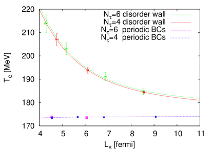
Figure 2: Estimate of finite volume corrections to the deconfinement temperature, set at 174 MeV for an infinite volume.

The infinite volume $T^{c}$ value (2), the lambda scale (12) and Eq. (11) give us the $g^{2}$ dependence of the lattice spacing $a$ in units of fermi. Using the $N_{\tau}=4$ fit to (III) of Fig. 1 together with Eqs. (1) and (6) allows to eliminate $g^{2}$ and we plot the resulting function $T^{c}(L_{s})$ in Fig. 2. Repeating this procedure for our $N_{\tau}=6$ fit to (III) gives, as is seen in Fig. 2, almost the same $T^{c}(L_{s})$ dependence and thus provides some evidence that our $N_{\tau}=4$ and 6 results are already representative for the finite volume continuum limit. For a box of volume $(10\,{\rm fermi})^{3}$ the pseudocritical temperature $T^{c}$ is about 5% higher than the infinite volume estimate and this correction increases to about 17% for a $(5\,{\rm fermi})^{3}$ box. For comparison we use the same procedure for analyzing the finite size dependence obtained by fitting the $N_{\tau}=4$ and 6 data with periodic BCs (including and enforcing the $\beta^{g}_{t}(6)=5.8941$ limit for $N_{\tau}=6$) to Eq. (22). This gives the two lower curves of the figure, which fall almost on top of one another. In that case error bars are considerably smaller than for the disorder wall data.

	Periodic BCs		Disorder wall BCs
$N_{s}$	$\chi_{\max}$	$\Delta\beta^{g}_{2/3}$	$\chi_{\max}$	$\Delta\beta^{g}_{2/3}$
12	3.585 (71)	0.0207 (11)	1.715 (27)	0.448 (18)
16	7.62 (16)	0.0103 (13)	1.879 (26)	0.0997 (21)
20	16.17 (67)	0.00498 (68)	2.525 (84)	0.0440 (27)
24	28.6 (1.1)	0.00277 (32)	3.58 (14)	0.0225 (16)
32	73.0 (2.0)	0.00132 (16)	7.67 (39)	0.00709 (61)

Table 3: Maxima of Polyakov loop susceptibility and width of the transition for lattices $4\times N_{s}^{3}$.

For a first order phase transition the maxima of the Polyakov loop susceptibility have to scale with the system volume to reproduce the delta function like singularity of a first order transition. For $N_{\tau}=4$ our $\chi_{\max}$ values are listed in table 3 and for $N_{\tau}=6$ in table 4. Using $N_{s}\geq 16$ for $N_{\tau}=4$ and $N_{s}\geq 20$ for $N_{\tau}=6$ acceptable fits to the straight-line form

$$\chi_{\max}=d_{1}+d_{2}\,(N_{s}/N_{\tau})^{3}$$ (24)

are obtained and shown together with their $Q$ values in Fig. 3 (for $N_{\tau}=6$ and periodic BCs only two data points are fitted, so that there is no $Q$ value in that case). To enhance the scale for the disorder wall fits, they are displayed on the right ordinate. The leading coefficients obtained from fits for disorder wall data differ from those for the data with periodic BCs: $d_{2}^{d}=0.01190\,(60)$ versus $d_{2}^{p}=0.1436\,(37)$ for $N_{\tau}=4$ and $d_{2}^{d}=0.00843\,(95)$ versus $d_{2}^{p}=0.0723\,(70)$ for $N_{\tau}=6$. This is possible because the Polyakov loop maxima are not physical observables, but bare quantities.

	Periodic BCs		Disorder wall BCs
$N_{s}$	$\chi_{\max}$	$\Delta\beta^{g}_{2/3}$	$\chi_{\max}$	$\Delta\beta^{g}_{2/3}$
18	2.47 (10)	0.0303 (21)	2.15 (20)	0.84 (04)
20	$-$	$-$	1.89 (10)	0.322 (25)
24	5.00 (27)	0.0162 (15)	1.90 (11)	0.140 (13)
28	$-$	$-$	2.18 (10)	0.0712 (69)
32	11.34 (55)	0.00803 (66)	2.82 (16)	0.0422 (37)
40	$-$	$-$	4.21 (31)	0.0234 (17)
48	$-$	$-$	5.44 (99)	0.0123 (38)

Table 4: Maxima of Polyakov loop susceptibility and width of the transition for lattices $6\times N_{s}^{3}$.

Figure 3: Maxima of Polyakov loop susceptibility.

Figure 4: The Polyakov loop susceptibility on a $4\times 16^{3}$ lattice with disorder wall BCs.

Let us now consider the width of the transition. For a $4\times 16^{3}$ lattice with disorder wall BCs the Polyakov loop susceptibility as a function of $\beta^{g}$ is shown in Fig. 4. We use reweighting FeSw88 ; BBook to cover a range of $\beta^{g}$ and define $\Delta\beta^{g}_{2/3}$ as the width of a peak at $2/3$ of its height. On large lattices the figures look less nice than Fig. 4, but provide still sufficient information to extract $\Delta\beta^{g}_{2/3}$. Our estimates for $N_{\tau}=4$ are listed in table 3 and for $N_{\tau}=6$ in table 4. The data are fitted to the form

$$\Delta\beta^{g}_{2/3}=c_{1}^{p}\left(\frac{N_{\tau}}{N_{s}}\right)^{3}+c_{2}^{p}\left(\frac{N_{\tau}}{N_{s}}\right)^{6}$$ (25)

for periodic BCs and to

$$\Delta\beta^{g}_{2/3}=c_{1}^{d}\left(\frac{N_{\tau}}{N_{s}}\right)^{3}+c_{2}^{d}\left(\frac{N_{\tau}}{N_{s}}\right)^{4}$$ (26)

for the disorder wall BCs. The first term reflects in both cases the delta function singularity of a first order phase transition. The leading order corrections to that differ due to the influence of the BCs.

Figure 5: Fits of the $N_{\tau}=4$ width of the transition.

For $N_{\tau}=4$ the final fits (see below) are shown in Fig. 5. From the disorder wall data we have omitted our smallest $4\times 12^{3}$ lattice from the fit, because the width becomes for it so broad that it spoils $Q$ (larger lattices than with periodic BCs are needed). The leading order coefficients are then $c_{1}^{p}=1.17\,(55)$ and $c_{1}^{d}=0.650\,(49)$. Both data sets together can still be consistently fitted using the weighted average $c_{1}=0.654\,(49)$ of the leading order coefficients and 1-parameter fits for $c_{2}$ in (25) and (26). This ensures that the ratio of the widths becomes one in the infinite volume limit. In contrast to the Polyakov loop maxima, the width of the transition is a physical observable, which is to leading order in the volume independent of the BCs. We have chosen to show these 1-parameter fits together with their $Q$ values in Fig. 5.

Figure 6: Fits of the $N_{\tau}=6$ width of the transition.

The methodology for the corresponding $N_{\tau}=6$ fits is the same as before. Using the data of table 4 we find the leading order coefficients $c_{1}^{p}=1.27\,(11)$ and $c_{1}^{d}=1.8\,(1.3)$, which average to $c_{1}=1.27\,(11)$. With this values consistent 1-parameter fits are obtained and together with their $Q$ values depicted in Fig. 6. Note that the ordinate scale in this figure is more than three times larger than in Fig. 5. Nevertheless the extracted physical values have to be the same to the extent that scaling holds.

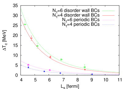
Figure 7: Estimate of finite volume correction to the width of the deconfinement phase transition.

We want to plot the width in physical units of MeV versus the box size in fermi and follow a similar procedure as before for $T^{c}(L_{s})$. For given $L_{s}(\beta^{g})$ we define

$$\Delta T^{c}(L_{s})=T(\beta^{g}_{pt}+\Delta\beta^{g}_{2/3}/2)-T(\beta^{g}_{pt}-\Delta\beta^{g}_{2/3}/2)\,.$$ (27)

The dependence $\Delta T(L_{s})$ is shown in Fig. 7. Compared to periodic BCs disorder wall BCs lead to a substantial broadening of the transition for the volumes considered: At $(10\,{\rm fermi})^{3}$ by a factor of 4.3 and at $(5\,{\rm fermi})^{3}$ by a factor of 5.5. The width is slightly less than 1% of the (enhanced) transition temperature at $(10\,{\rm fermi})^{3}$ and about 8% at $(5\,{\rm fermi})^{3}$. Within the error bars, which are quite large for the widths, scaling works again well.

Simulations with disorder wall BCs have turned out to be far more CPU time consuming than those with periodic BCs. The decreased heights of our pseudo-transition signals (the maxima of the Polyakov loop susceptibilities), their increased widths and the strong finite size effects are the underlying reasons. While the reweighting range FeSw88 ; BBook is about the same for simulations with periodic or disorder wall BCs on identically sized lattices, accurate disorder wall results require far more patches, i.e., independent simulations at distinct $\beta^{g}$ values. In addition the signal is worse due to the decreased heights of the peaks. Finally extrapolations to infinite lattices, as needed for the finite volume continuum limit, are more demanding due to the strong and more sophisticated finite size corrections. This is helped by including infinite volume extrapolations from periodic lattices as disorder wall data points, what can be done because these extrapolations do not depend on the BCs. Still, data from our largest $6\times 48^{3}$ lattice turn out to be essential to stabilize the $N_{\tau}=6$ fits for large lattice sizes. Far smaller lattices are sufficient when periodic BCs are used.

IV Summary and Conclusions

Relatively small physical volumes as typical for the deconfined phase in BNL RHIC RHIC lead in our SU(3) investigation to a substantial rounding of the transition and to an increase of the (effective) deconfinement temperature by 5% to 20%. The physical reason for these corrections is that correlation lengths are proportional to $L_{\tau}$ and $L_{\tau}/L_{s}$ does not approach zero in the finite volume continuum limit. We estimate that the corrections are negligible for the geometry of a torus, used in practically all previous LGT simulations of the subject, but not for BCs which reflect the cold exterior. Using the disorder wall BCs introduced in section II.1, we find the magnitude of the effects on pure SU(3) LGT competitive to those of other corrections, foremost the inclusion of quarks. In particular the width of the transition increases by factors 4 to 6 over the width found for a torus of the same physical size.

Most scattering events at a RHIC are not from central collisions. So one has to cope with a distribution of volumes, each of it associated with its own effective deconfinement temperature and width. Due to such finite volume effects the concept of a sharp transition becomes blurred even when the effects of quarks, which convert the transition into a crossover Ao06 , are not yet taken into account. Ultimately one may want to extend LGT studies of the deconfining transition with BCs reflecting the confined outside world to full QCD. Before doing so, additional experience can be gained from pure SU(3) LGT. In future work we intend to perform simulation for the physically more realistic confinement wall BCs, which we introduced in section II.2. Further, the entire equilibrium thermodynamics of the deconfined phase ought to be addressed.

Close to the transition point the deconfined phase can only be studied non-perturbatively. Equilibrium QCD on the lattice allows this from first principles. But the assumption that equilibrium configurations can capture the essence of the transition is a strong one. Studies of the important dynamical aspects of the transition have to rely on phenomenological approaches. For instance, models which use hydrodynamics in the quark gluon plasma stage reproduce experimental data on particle abundances and flows well pheno .

- (1) L.D. McLerran and B. Svetitsky, Phys. Lett. B 98, 195 (1981); J. Kuti, J. Polónyi, and K. Szlachányi, Phys. Lett. B 98, 199 (1981).
- (2) P. Petreczky, Nucl. Phys. B (Proc. Suppl.) 140, 78 (2005); E. Laermann and O. Philipsen, Ann. Rev. Nucl. Part. Sci. 53, 163 (2003).
- (3) We omit the adverb “quantum” in front of continuum limit from hereon. The classical continuum limit is not considered in our paper.
- (4) H.J. Rothe, Lattice Gauge Theories: An Introduction, 3rd edition, World Scientific, Singapore 2005.
- (5) Often the physical scale in pure gauge calculations is set by choosing a value of about 420 MeV for the string tension , which then leads via scaling to MeV. However, in this paper we prefer to deal with a value close to its physical QCD estimate, as one is ultimately interested in corrections to this value.
- (6) For a review see, e.g., B. Muller, J.L. Nagle, Ann. Rev. Nucl. and Part. Sci. 56, 93 (2006)
- (7) A. Bazavov, B. Berg, and A. Velytsky, Phys. Rev. D 74, 014501 (2006).
- (8) Eq. (19) of Ba06 .
- (9) A. Hurwitz, Göttinger Gesellschaft der Wissenschaften 1897, 71 (1897).
- (10) A. Haar, Ann. Math. 34, 147 (1933).
- (11) F. Brown, N. Christ, Y. Deng, M. Gao, and T. Woch, Phys. Rev. Lett. 61, 2058 (1988); M. Fukugita, M. Okawa, A. Ukawa, Phys. Rev. Lett. 63, 1768 (1989); N.A. Alves, B.A. Berg, and S. Sanielevici, Phys. Rev. Lett. 64, 3107 (1990).
- (12) D.J. Gross and F. Wilczek, Phys. Rev. Lett. 30, 1343 (1973); H.D. Politzer, Phys. Rev. Lett. 30, 1346 (1973).
- (13) G. Boyd, J. Engels, F. Karsch, E. Laermann, C. Legeland, M. Lütgemeier, and B. Petersson, Nucl. Phys. B 469, 419 (1996).
- (14) J. Kogut, R. Pearson, and J. Shigemitsu, Phys. Rev. Lett. 43, 484 (1979); G. Münster and P. Weisz, Phys. Lett. B 96, 119 (1980).
- (15) G. Münster, Nucl. Phys. B 190 [FS3], 439 (1981); Erratum 200 [FS4], 536 (1982).
- (16) F. Karsch, Nucl. Phys. B 205 [FS5], 285 (1982).
- (17) This follows from Eq. (1.4) of Ka82 . Note that in that equation in the continuum limit due to Eq. (2.4) of Ka82 .
- (18) B.A. Berg, Markov Chain Monte Carlo Simulations and Their Statistical Analysis, World Scientific, Singapore, 2004.
- (19) A.M. Ferrenberg and R.H. Swendsen, Phys. Rev. Lett. 61, 2635 (1988); erratum 63, 1658 (1989).
- (20) Y. Aoki, G. Endródi, Z. Fodor, S.D. Katz, and K.K. Szabó, Nature 443, 675 (2006).
- (21) D. Teaney, J. Lauret, and E.V. Shuryak, Phys. Rev. Lett. 86, 4783 (2001); T. Hirano and M. Gyulassy, Nucl. Phys. A 769, 71 (2006).