QCD phase diagram: an overview

Abstract:

The aim of this review is to summarize the contemporary understanding of the QCD phase diagram as a function of temperature $T$ and baryo-chemical potential $\mu_{B}$. The focus is on recent theoretical developments due to lattice simulations of the phase diagram.

1 Introduction

Quantum Chromodynamics is a remarkable theory. It is a convincing practical example of the triumph of the quantum field theory. Asymptotic freedom allows QCD to be consistent down to arbitrary short distance scale, enabling us to define the theory completely in terms of the fundamental microscopic degrees of freedom – quarks and gluons. This fundamental definition is very simple, yet the theory describes a wide range of phenomena – from the mass spectrum of hadrons to deep-inelastic processes. As such, QCD should also possess well defined thermodynamic properties. The knowledge of QCD thermodynamics is essential for the understanding of such natural phenomena as compact stars and laboratory experiments involving relativistic heavy-ion collisions.

Full analytical treatment of QCD is very difficult because, neglecting quark masses, this theory has no numerically small fundamental parameters. The only independent intrinsic scale in this theory is the dynamically generated confinement scale $\Lambda_{\rm QCD}\sim 1{\rm fm}^{-1}$. In certain limits, in particular, for large values of the external thermodynamic parameters temperature $T$ and/or baryo-chemical potential $\mu_{B}$, when thermodynamics is dominated by short-distance QCD dynamics, the theory can be studied analytically, due to the asymptotic freedom. But, as seen below, the most interesting experimental region of parameters $T$ and $\mu_{B}$ is that of order $\Lambda_{\rm QCD}$.

The above makes first principle lattice approaches, which do not rely on small parameter expansions, an invaluable and the most powerful tool in studying QCD thermodynamics. In addition, the domain where all relevant time/distance (or energy/momentum) scales are similar is especially suited for a lattice study (accommodating a wide scale window would require a correspondingly large lattice).

The full potential of lattice methods is close to being realized as far as the study of QCD at $\mu_{B}=0$ is concerned. The main practical problems in this regime – accommodating sufficiently light quarks and approaching the continuum limit – are being methodically and successfully addressed through the use of improved lattice discretization schemes, as well as advances in algorithm and hardware technology.

The status of thermodynamics of QCD at non-zero $\mu_{B}$ is different. The main impediment to lattice simulations is the notorious sign problem, discussed in Section 3.1. No method devised so far is known, or expected, to converge to the correct physical result as the infinite volume limit is approached at fixed $\mu_{B}\neq 0$. However, since the most interesting structure of the QCD phase diagram (phase transitions and critical points) lie at nonzero $\mu_{B}$, any progress in this direction is especially valuable. Existing lattice methods generically rely on clever extrapolations from $\mu_{B}=0$. These techniques yield interesting results in the regime of small, but already experimentally relevant $\mu_{B}$.

A contemporary view of the QCD phase diagram is shown in Fig. 3. It is a compilation of a body of results from model calculations, empirical nuclear physics, as well as first principle lattice QCD calculations and perturbative calculations in asymptotic regimes.

Several reviews in these proceedings, in addition to original contributions, are devoted to recent progress in lattice studies of QCD thermodynamics. Ref. [1] reviews thermodynamics of QCD at $\mu_{B}=0$. Ref. [2] discusses lattice results at small $\mu_{B}$. In addition, Ref.[3] describes resent progress in uncovering phase structure of QCD at large $\mu_{B}$, relevant to the physics of compact stars, and outlines targets of opportunity for potential future lattice studies in this domain.

This report provides an overview of the structure of the QCD phase diagram based on available theoretical (lattice and model calculations) and phenomenological input. Some of the recent lattice results reported separately in this volume are also briefly discussed in Section 4.

2 The phase diagram

Thermodynamic properties of a system are most readily expressed in terms of a phase diagram in the space of thermodynamic parameters – in the case of QCD – as a $T\mu_{B}$ phase diagram. Each point on the diagram corresponds to a stable thermodynamic state, characterized by various thermodynamic functions, such as, e.g., pressure, baryon density, etc (as well as kinetic coefficients, e.g., diffusion or viscosity coefficients, or other properties of various correlation functions).

Static thermodynamic quantities can be derived from the partition function – a Gibbs sum over eigenstates of QCD Hamiltonian, which can be alternatively expressed as a path integral in Euclidean space:

$$Z(T,\mu_{B})=\sum_{\alpha}\exp\left\{-\frac{E_{\alpha}-\mu_{B}B_{\alpha}}{T}\right\}=\int{\cal D}(A,q,q^{\dagger})\exp\left\{-S_{E}\right\}$$ (1)

where $\alpha$ labels states with energy $E_{\alpha}$ and baryon number $B_{\alpha}$. The path integral is over color gauge (gluon) fields $A_{\mu}$ periodic in Euclidean time with period $1/T$, and quarks fields, antiperiodic with the same period. The Euclidean action given by

$$S_{E}=S_{\rm YM}+\sum_{q=u,d,s}\int d^{4}x\ q^{\dagger}\,\mathbb{D}\,q$$ (2)

where $S_{\rm YM}[A]$ is the SU(3) Yang-Mills action and, in the chiral Weyl basis, the Dirac spinors and matrix are

$$q=\left(\begin{array}[]{c}q_{L}\\ q_{R}\end{array}\right)\quad{\rm and}\quad\mathbb{D}=\left(\begin{array}[]{cc}\sigma\cdot D&m_{q}\\ m_{q}&\sigma^{\dagger}\cdot D\\ \end{array}\right)-\mu_{q}$$ (3)

where $\sigma_{\mu}=(1,i\boldsymbol{\sigma})$, $D_{\mu}=\partial_{\mu}-iA_{\mu}$, and $\mu_{q}=\mu_{B}/3$.

2.1 Chiral symmetry argument

In the chiral limit – the idealized limit when 2 lightest quarks, $u$ and $d$, are taken to be massless, the Lagrangian of QCD acquires chiral symmetry SU(2)${}_{L}\times$SU(2)_R, corresponding to SU(2) flavor rotations of $(u_{L},d_{L})$ and $(u_{R},d_{R})$ doublets independently. The ground state of QCD breaks the chiral symmetry spontaneously locking SU(2)_L and SU(2)_R rotations into a single vector-like SU(2)_V (isospin) symmetry and generating 3 massless Goldstone pseudoscalar bosons – the pions. The breaking of the chiral symmetry is a non-perturbative phenomenon.

At sufficiently high temperature $T\gg\Lambda_{\rm QCD}$, due to the asymptotic freedom of QCD, perturbation theory around the approximation of the gas of free quarks and gluons (quark-gluon plasma – QGP) should become applicable. In this regime chiral symmetry is not broken. Thus we must expect a transition from a broken chiral symmetry vacuum state to a chirally symmetric equilibrium state at some temperature $T_{c}\sim\Lambda_{\rm QCD}$. The transition is akin to the Curie point in a ferromagnet – where the rotational O(3) symmetry is restored by thermal fluctuations (chiral O(4)=SU(2)$\times$SU(2) symmetry in QCD). Thermodynamic functions of QCD must be singular at the transition point – as always when the transition separates thermodynamic states of different global symmetry.

Thus, the region of broken chiral symmetry on the $T\mu_{B}$ phase diagram must be separated from the region of the restored symmetry by a closed boundary as shown in Fig. 1.

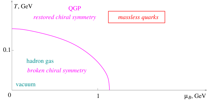
Figure 1: Phase diagram of QCD with massless quarks dictated by the chiral symmetry argument. The order of the transition (solid magenta line) is not determined by this simplest argument.

2.2 Pisarski-Wilczek argument

The chiral symmetry argument alone is not sufficient to determine the order of the temperature driven chiral symmetry restoration transition. A more elaborate argument, based on universality, advanced by Pisarski and Wilczek [4] asserts that the transition cannot be of second order for three massless quarks.

In a simplified form, the logic of Ref.[4] is as follows. Let us assume that the transition is of the second order. Then the critical behavior of the system (long-distance behavior of correlation functions, singular contributions to thermodynamic functions, etc.) is determined by the long-wavelength modes which, in the case of the second order transition in a theory with $N_{\rm f}$ light quarks, are the $N_{\rm f}^{2}-1$ pions of the spontaneously broken SU$(N_{\rm f})_{A}$ axial flavor symmetry plus the critical mode – the magnitude of the chiral condensate $\sigma\sim\bar{q}q$.

Universality implies that the critical behavior is the same as in any local theory in 3 dimensions with the same global symmetry breaking pattern and the same set of critical modes. In our case, a representative example of the universality class is an SU($N_{\rm f}$)$\times$ SU($N_{\rm f}$) sigma model of an $N_{\rm f}\times N_{\rm f}$ matrix-valued field $\Phi$. It turns out, that for $N_{\rm f}=3$, the model cannot be critical: there is a relevant operator cubic in the order parameter field, $\det\Phi$, which always destabilizes the symmetric minimum of the effective potential for $\Phi$ via a first order transition, before the curvature of the minimum vanishes (i.e., before criticality is reached). Hence, QCD with $N_{\rm f}=3$ massless quark flavors must undergo a first order chiral restoration transition.

2.3 $N_{\rm f}=2$ chiral limit and tricritical point

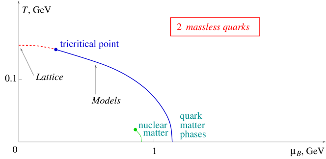
Figure 2: The order of the chiral symmetry restoration transition for 2 massless and one massive quarks. The dashed line (red) is the second order transition, the solid line (blue) is the first order transition. In the low $T$ region: chiral symmetry is broken in nuclear matter. Details of the phase structure at high $\mu_{B}$ are omitted.

For two massless quarks the transition can be either second or first order. As lattice and model calculations show, both possibilities are realized depending on the value of the strange quark mass $m_{s}$ and/or the baryo-chemical potential $\mu_{B}$.

The point on the chiral phase transition line where the transition changes order is called tricritical point, see Fig. 2. The location of this point is one of the unknowns of the QCD phase diagram with 2 massless quarks. In fact, even the order of the transition at $\mu_{B}=0$, which many older and recent studies suggest is of the second order (as shown in Fig. 2) is still being questioned (see review by Heller in this volume [1]).

Neither can it be claimed reliably (model or assumption independently) that the transition, if it begins as a 2nd order at $\mu_{B}=0$, changes to first order. However, numerous model calculations show this is the case (Section 3.4). Lattice calculations also support such a picture. Recent advances in the understanding of QCD at low $T$ and large $\mu_{B}$, reviewed in [3], also point at a first order transition (at low-$T$, high-$\mu_{B}$) from nuclear matter to color-superconducting quark matter phase. Fig. 2 reflects this consensus.

At low temperature, nuclear matter (which is expected to be still bound in the chiral limit) should be placed on the broken symmetry side of the chiral transition line as shown in Fig. 2.

2.4 Physical quark masses and crossover

When the up and down quark masses are set to their observed finite values, the diagram assumes the shape sketched in Fig. 3. The second order transition line (where there was one) is replaced by a crossover – the criticality needed for the second order transition in Fig. 2 requires tuning chiral symmetry breaking parameters (quark masses) to zero. In the absence of the exact chiral symmetry (broken by quark masses) the transition from low- to high-temperature phases of QCD need not proceed through a singularity. Lattice simulations do indeed show that the transition is a crossover for $\mu_{B}=0$ (most recently and decisively Ref.[5], see also Ref.[1] for a review).

This transitional crossover region is notoriously difficult to describe or model analytically – description in terms of the hadronic degrees of freedom (resonance gas) breaks down as one approaches crossover temperature (often called $T_{c}$), and the dual description in terms of weakly interacting quarks and gluons does not become valid until much higher temperatures. Recent terminology for the QCD state near the crossover ($T\sim(1-2)T_{c}$) is strongly coupled quark-gluon plasma (sQGP).

Transport properties of sQGP have attracted considerable attention. For example, generally, the shear viscosity $\eta$ is a decreasing function of the coupling strength. The dimensionless ratio of $\eta/\hbar$ to the entropy density $s$ tends to infinity asymptotically far on either side of the crossover – in dilute hadron gas ($T\to 0$) and in asymptotically free QGP ($T\to\infty$). Near the crossover $\eta/s$ should thus be expected to reach a minimum [6]. The viscosity can be indirectly determined in heavy ion collisions by comparing hydrodynamic calculations to experimental data. Such comparison [7] indeed indicates that the viscosity (per entropy density) of this “crossover liquid” is relatively small, and plausibly is saturating the lower bound conjectured in [8].

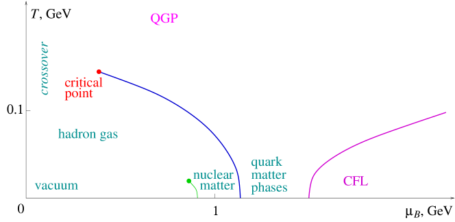
Figure 3: The contemporary view of the QCD phase diagram – a semiquantitative sketch.

2.5 Physical quark masses and the critical point

The first order transition line is now ending at a point known as the QCD critical point or end point. The end point of a first order line is a critical point of the second order. This is by far the most common critical phenomenon in condensed matter physics. Most liquids possess such a singularity, including water. The line which we know as the water boiling transition ends at pressure $p=218$ atm and $T=374^{\circ}$C. Along this line the two coexisting phases (water and vapor) become less and less distinct as one approaches the end point (the density of water decreases and of vapor increases), resulting in a single phase at this point and beyond.

In QCD the two coexisting phases are hadron gas (lower $T$), and quark-gluon plasma (higher $T$). What distinguishes the two phases? As in the case of water and vapor, the distinction is only quantitative, and more obviously so as we approach the critical point. Since the chiral symmetry is explicitly broken by quark masses, the two phases cannot be distinguished by realizations (broken vs restored) of any global symmetry.

It is worth pointing out that beside the critical point, the phase diagram of QCD in Fig. 3 has other similarities with the phase diagram of water. A number of ordered quark matter phases must exist in the low-$T$ high-$\mu_{B}$ region, which are akin to many (more than 10) confirmed phases of ice. For asymptotically large $\mu_{B}$, QCD with 3 quark flavors must be in color-flavor locked (CFL) state [9, 3].

3 Locating the critical point: theory

The critical point is a well-defined singularity on the phase diagram, and it appears as an attractive theoretical, as well as experimental, target to shoot at. Theoretically, finding the coordinates $(T,\mu_{B})$ of the critical point is a straightforwardly defined task. We need to calculate the partition function of QCD given by Eq. (1) and find the singularity corresponding to the end of the first order transition line. But it is easier said than done.

Of course, calculating such an infinitely dimensional integral analytically is beyond present reach. Numerical lattice Monte Carlo simulations is an obvious tool to choose for this task. At zero $\mu_{B}$ Monte Carlo method allows us to determine the equation of state of QCD as a function of $T$ (and show that the transition is a crossover). However, at finite $\mu_{B}$ the Nature guards its secrets better.

3.1 Importance sampling and the sign problem

The notorious sign problem has been known to lattice Monte Carlo experts since the early days of this field. Calculating the partition function using Monte Carlo method hinges on the fact that the exponent of the Euclidean action $S_{E}$ is a positive-definite function of its variables (values of the fields on the lattice). This allows one to limit calculation to a relatively small set of field configurations randomly picked with probability proportional to the value of $\exp(-S_{E})$. The number of such configurations needed to achieve reasonable accuracy is vastly smaller than the total number of possible configurations. The latter is exponentially large in the size $V$ of the system, or, the number of the degrees of freedom: $\exp(\operatorname{const}\cdot V)$. The method, also known as importance sampling, utilizes the fact that the vast majority of these configurations contribute a tiny fraction because of the exponential suppression by $\exp(-S_{E})$. Only configurations with sizable $\exp(-S_{E})$ are important.

In QCD with $\mu_{B}\neq 0$ the Monte Carlo action $S_{\rm MC}$ (playing the role of $S_{E}$) is complex. With $S_{\rm MC}$ complex, how does one pick important configurations? A number of ways to circumvent the problem have been tried. For example, using the modulus of $\exp(-S_{\rm MC})$ as a measure of importance, or the value of $\exp(-S_{\rm MC})$ at zero $\mu_{B}$, when it is still positive. Unfortunately, none of the methods can be expected to converge to correct result with the increasing lattice volume, unless this limit is not accompanied by an exponential $\exp(\operatorname{const}\cdot V)$ increase of the number of configurations, rendering Monte Carlo technique useless.

3.2 The overlap problem

To demonstrate the problem, consider the most straightforward attempt to circumvent it – reweighting. We cannot obtain a correctly weighted sample of important configurations directly at $\mu_{B}\neq 0$. But we still can at $\mu_{B}=0$. So, we take the $\mu_{B}=0$ sample and offset incorrect probability by multiplying the contribution of each configuration by a factor $\exp(+S_{E}|_{\mu_{B}=0}-S_{E})$. This is exact in the limit when the sample contains all possible configurations.

The problem is in the size of the sample needed for a Monte Carlo computation as $V\to\infty$. The method uses the fact that at finite volume $V$, even at $\mu_{B}=0$, the configurations important for ${\mu_{B}\neq 0}$ pop up, but with a very small probability. This probability is exponentially small as volume $V\to\infty$: $\exp(-{\rm const}\cdot V)$. When we calculate the partition function the reweighting factor is correcting for that, and is therefore exponentially large (for the complex $S_{\rm MC}$, both he magnitude and the complex phase are). Fluctuations, or statistical noise, in the exponentially tiny number of the rare important configurations completely washes out the significance of the result.

In layman’s terms, imagine that we want to study ice, but can only run experiments at normal room temperature and pressure. Using the reweighting method is analogous to trying to glimpse the information by waiting for rare configurations when all the water molecules accidentally gather in one corner of the lab, forming a chunk of ice. The amount of time that this experiment would require is exponentially large as $V\to\infty$.

3.3 Complex determinant

Why is the Monte Carlo action in QCD complex and what can be done about it? To see, integrate over the quark fields in (1) explicitly and obtain

$$Z=\int{\cal D}A\ e^{-S_{\rm YM}}\prod_{q}\det\mathbb{D}\equiv\int{\cal D}A\ e^{-S_{\rm MC}}$$ (4)

where (as in Eq. (3) and using the property $D^{\dagger}=-D$):

$$\mathbb{D}=\left(\begin{array}[]{cc}\sigma\cdot D-\mu_{q}&m_{q}\\ m_{q}&-(\sigma\cdot D)^{\dagger}-\mu_{q}\\ \end{array}\right)$$ (5)

For $\mu_{q}=0$ each quark determinant in Eq. (4) is manifestly positive:

$$\det\mathbb{D}=\det[(\sigma\cdot D)(\sigma\cdot D)^{\dagger}+m_{q}^{2}]>0.$$ (6)

The positivity (and even reality) is lost if $\mu_{q}\neq 0$. This is the sign problem.

However, the following still holds $(\det\mathbb{D}(\mu_{q}))^{*}=\det\mathbb{D}(-\mu_{q}^{*})$. This opens two possibilities for the measure in the Euclidean path integral (4) to remain positive for $\mu_{q}\neq 0$: (a) if $\mu_{q}$ is imaginary; or (b) if there are two degenerate quarks, e.g., $m_{u}=m_{d}$ and $\mu_{u}=-\mu_{d}$, which is what happens with the chemical potential $\mu_{I}$ of isospin $I_{3}$, or in phase-quenched QCD. Both alternatives are being exploited to glimpse into the regime $\mu_{B}\neq 0$, yet unaccessible to direct Monte Carlo. In particular, the recent results from the simulations at finite $\mu_{I}$ are reported in Ref.[11]. Simulations at imaginary $\mu_{B}$ are discussed further in Section 4.2.

3.4 Predictions from models

In the absence of a controllable (i.e., systematically improvable and converging in the $V\to\infty$ limit) method to simulate QCD at nonzero $\mu_{B}$, one turns to model calculations. Many such calculations have been done [12, 13, 14, 15, 16, 17, 18, 19, 20, 21]. Figure 4 summarizes the results. One can see that the predictions vary wildly. An interesting point to keep in mind is that each of these models is tuned to reproduce vacuum, $T=\mu_{B}=0$, phenomenology. Nevertheless, extrapolation to nonzero $\mu_{B}$ is not constrained significantly by this. In a loose sense, most lattice methods (see next Section) can be also viewed as extrapolations from $\mu_{B}=0$, albeit with reliable input from finite $T$.

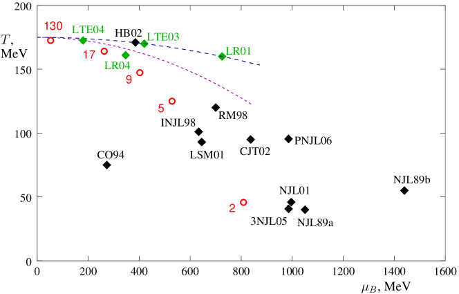
Figure 4: Comparison of predictions for the location of the QCD critical point on the phase diagram. Black points are model predictions: NJLa89, NJLb89 – [12], CO94 – [13, 14], INJL98 – [15], RM98 – [16], LSM01, NJL01 – [17], HB02 – [18], CJT02 – [19], 3NJL05 – [20], PNJL06 – [21]. Green points are lattice predictions: LR01, LR04 – [22], LTE03 – [23], LTE04 – [24]. The two dashed lines are parabolas with slopes corresponding to lattice predictions of the slope $dT/d\mu_{B}^{2}$ of the transition line at $\mu_{B}=0$ [23, 25]. The red circles are locations of the freezeout points for heavy ion collisions at corresponding center of mass energies per nucleon (indicated by labels in GeV) – Section 5.

4 Lattice results on the critical point

This section is devoted to brief (and necessarily incomplete) descriptions of currently developed lattice methods for reaching out into the $T\mu_{B}$ plane. The comments below are selective and are meant to complement the original contributions in this volume. For a more comprehensive description of these methods, as well as other methods not discussed here, the reader may consult the most up-to-date review of Schmidt in these proceedings [2] as well as an earlier review by Philipsen [26], both of which also contain further references to original papers.

4.1 Reweighting

The first lattice prediction for the location of the critical point was reported by Fodor and Katz in Ref. [22]. The assumption is that, although the problem becomes exponentially difficult as $V\to\infty$, in practice, one can get a sensible approximation at finite $V$. In addition, simulations at finite $T$ might suffer lesser overlap problem because of large thermal fluctuations [27]. One can hope that if the critical point is at a small value of $\mu_{B}$, the volume $V$ may not need to be too large to achieve a reasonable accuracy. In particular, numerical estimates show [28] that the maximal value of $\mu_{B}$ which one can reach within the same accuracy shrinks only as a power of $1/V$.

The results of Ref. [22] are the most definitive and well-known, but they also attract the strongest of criticisms. The method of the Ref. [22] is based on computing the position of the zero of the partition function in the complex temperature plane and observing when (for which $\mu_{B}$) this zero crosses (and with its complex conjugate – pinches) the real axis. This determines the $T$ and $\mu_{B}$ coordinates of the critical point. However, as Ejiri points out in Ref. [29], once the fluctuations of the phase, $\arg\det{\mathbb{D}}$, of the Dirac determinant are large, they cause fake zeros to appear. It is therefore alarming that, as Splittorff argues [30], both points found in Ref. [22] (different $m_{q}$ and $V$) happen to lie on the critical line of the phase quenched QCD ($|\det{\mathbb{D}}|$ instead of $\det{\mathbb{D}}$) – which is the line where fluctuations of $\arg\det{\mathbb{D}}$ do become large. In a related observation, Golterman et al [31, 32] argue that the procedure of taking the fourth root [33] of the staggered fermions causes problems in a finite $\mu_{B}$ calculation such as in Ref.[22].

4.2 Imaginary $\mu_{B}$ and $N_{\rm f}=3$

By the universality argument of Section 2.2, the finite temperature transition is 1st order for $m_{u}=m_{d}=m_{s}=0$. By continuity, it must remain 1st order in a finite domain of the $m_{s}m_{ud}$ plane (taking $m_{u}=m_{d}=m_{ud}$) surrounding the origin – the plot of this domain is known as Columbia plot [34, 1]. For physical quark masses and $\mu_{B}=0$ the temperature driven transition is a crossover, which means that the physical point is outside the 1st order domain in the $m_{s}m_{ud}$ plot. Reducing quark masses should pull the point into the 1st order domain.

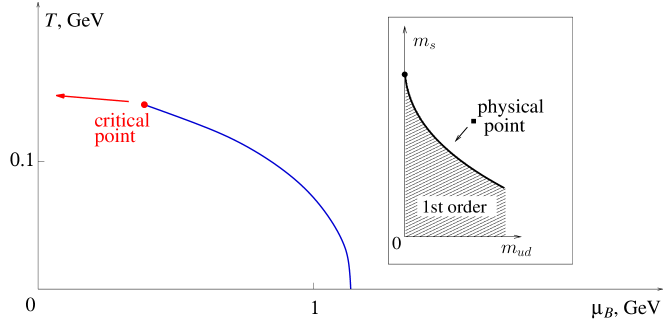
Figure 5: Expected direction of motion of the critical point (left) as the quark masses are decreased as shown in the Columbia plot in the inset.

What happens on the $T\mu_{B}$ phase diagram as the point $m_{s}m_{ud}$ is pulled towards and into the first order domain? The most straightforward expectation is that the first order line begins earlier, at lower $\mu_{B}$, i.e., the critical point is pulled towards the $\mu_{B}=0$ axis, as shown in Fig. 5, until it disappears off the phase diagram altogether, and the whole transition line is of the 1st order. Furthermore, lattice calculations at $\mu_{B}=0$ show that real QCD is very near the 1st order domain boundary. That suggests the critical point is not too far off the $T$ axis in the $T\mu_{B}$ plane.

What happens to the critical point when $(m_{s},m_{ud})$ is in the 1st order domain? It is still a singularity of the partition function as a function of $\mu_{B}$, but it moves out into the complex $\mu_{B}$ plane. More precisely, it moves to imaginary $\mu_{B}$ axis. This remarkable fact allows one to observe the (complex descendant of) the critical point in a direct Monte Carlo simulation – since there is no sign problem for imaginary $\mu_{B}$ (Section 3.3). This observation is at the core of the method developed by de Forcrand and Philipsen [25, 35].

The success of the method crucially depends on the analyticity of the coordinate $\mu_{B}^{2}$ of the critical point as a function of quark mass, e.g., $m_{s}$ around the point where $\mu_{B}^{2}=0$. The validity of this can be argued as follows. In the $(T,\mu_{B},m_{s})$ space the criticality is achieved (correlation length goes to infinity) when 2 conditions are satisfied: $t(T,\mu_{B}^{2},m_{s})=h(T,\mu_{B}^{2},m_{s})=0$, i.e., there are two relevant operators in the universality class of the critical point and their coefficients, $t$ and $h$, must be tuned to zero. The coefficients of these operators are analytic functions of the parameters. Furthermore, the analyticity in $\mu_{B}^{2}$ (not just in $\mu_{B}$, which otherwise could cause a branching point at $\mu_{B}^{2}=0$) follows from the $\mu_{B}\to-\mu_{B}$ symmetry of the QCD partition function. Solving the two conditions for $T$ and $\mu_{B}^{2}$ one finds the position of the critical point $(T(m_{s}),\mu_{B}^{2}(m_{s}))$ in terms of functions analytic in $m_{s}$.

de Forcrand and Philipsen determine the function $\mu_{B}^{2}(m_{s})$, or rather its inverse $m_{s}(\mu_{B}^{2})$, for $\mu_{B}^{2}<0$ and then analytically continue to real $\mu_{B}$. This way one could estimate the position of the critical point in the $T\mu_{B}$ plane.

It is puzzling that the slope of the function $m_{s}(\mu_{B}^{2})$ measured in this way [25, 35] appears negligible in lattice units and has a wrong sign after a translation to physical units is applied. This leads the authors of Refs. [25, 35] to suggest an unusual scenario: a new critical point is emerging on the phase diagram as the $(m_{s},m_{ud})$ point is taken into the 1st order domain on the Columbia plot, dragging a new line of 1st order transitions into the $T\mu_{B}$ plane. An unusual feature of such a point worth pointing out is the positioning of the 1st order line on the high temperature side of the critical point. As emphasized in Ref.[35], these results should still be subject to large uncertainties due to discretization and/or finite volume errors and more refined simulations are needed before physical conclusions can be drawn.

4.3 Taylor expansion

Taylor expansion in $\mu_{B}$ is another method to circumvent the sign problem. Derivatives of pressure (or other thermodynamic quantities) are calculated at $\mu_{B}=0$ and assembled into a Taylor series expansion to obtain dependence of that quantity on $\mu_{B}$ [23, 24, 36]

Consistent with the existence of the critical point at finite $\mu_{B}$, there is a noticeable rise in the baryon number susceptibility $\chi_{B}$ – see the peak on Fig. 6. Such a peak should be expected since the baryon number susceptibility diverges at the critical point. On the other hand, the isospin susceptibility should not diverge at the critical point, because the critical mode, $\sigma\sim\bar{q}q$ is an isoscalar and cannot be excited by the operator of isospin $I_{3}$ (while it is excitable by the operator of the baryon number).

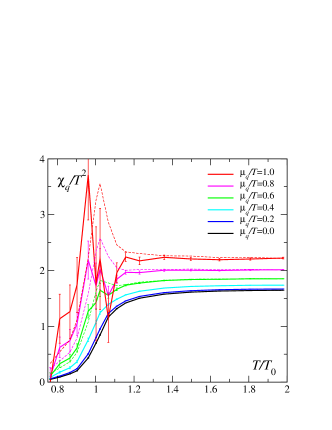
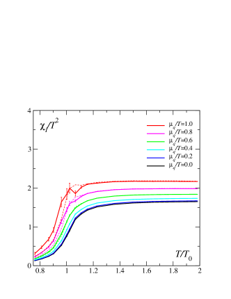
Figure 6: Allton, et al [37]: peak in baryon number susceptibility $\chi_{B}=9\chi_{q}$ (left), but not in isospin susceptibility $\chi_{I}$ (right). See Ref.[2] for updated figure.

The authors of Ref. [37] caution against attributing the peak to the critical point. Their reservation is due to the fact that the low-$T$ side of the peak is well described by a hadronic resonance gas model. Nevertheless, the agreement with the resonance gas does not necessarily mean that the rise of susceptibility cannot be due to the critical point of QCD. On the contrary, viewing resonance gas conceptually as a complementary (dual) description of QCD one must conclude that resonance description must reproduce the same thermodynamic functions as fundamental QCD description – including the critical point. Although the simple resonance gas model used in Ref.[37] does not describe the critical point itself, it still might be describing the onset of the critical behavior, just before the model breaks down.

Furthermore, the resonance gas model of Ref.[37] does not describe the higher $T$ side of the peak. The model must break down as the peak is approached from below, and is certainly not valid above the peak, where a different description must be used. At the same time, both sides of the peak receive a natural interpretation in terms of the proximity of the critical point.

4.4 Radius of convergence of the Taylor expansion

At a fixed temperature, the convergence radius of the Taylor expansion in $\mu_{B}$ is limited by the nearest singularity in the complex plane of $\mu_{B}$. Assuming that at the temperature $T_{E}$, at which the critical point $(T_{E},\mu_{E})$ occurs on the phase diagram, this critical point is the nearest singularity to $\mu_{B}=0$, one could use Taylor expansion to determine $\mu_{E}$ [23, 24, 36, 2], if $T_{E}$ is known.

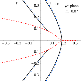
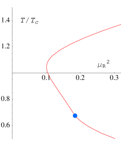
Figure 7: Ref[38]: The location of complex plane singularities (cuts in the thermodynamic limit)) in the random matrix model at two representative values of $T$: $T_{c}$ and $T_{E}$. At $T_{E}$ the branching points pinch the real axis – this is where the critical point appears on the phase diagram. The trajectories of the branching points are shown by a dashed (red) curve. On the right the radius of convergence of the Taylor series, set by the distance from $\mu_{B}=0$ to the branching point, is plotted as a function of $T$ (the latter is along the ordinate to facilitate the comparison with QCD phase diagram). The critical point is shown.

Assuming that the radius of convergence $\mu_{R}$ can be approximated using the first few terms of the Taylor expansion, one can plot $\mu_{R}$ as a function of $T$. The main remaining problem is to determine the value of $T_{E}$ i.e., to identify at which value of $T$ the complex singularity reaches the real axis in the $\mu_{B}$ plane. This question has been addressed using universality arguments, as well as an example random matrix calculation in Ref[38]. The trajectory of the complex singularities is illustrated in Fig. 7.

Two conclusions can be made: (i) The minimum value of the radius of convergence is not achieved at $T=T_{E}$, but rather at a temperature close to the temperature $T_{c}$ of the chiral transition at $\mu_{B}=0$. (ii) At $T_{E}$ the function $\mu_{R}(T)$ has a high order singularity.

It is unlikely that such a weak singularity alone can be used to identify the value of $T_{E}$. This suggests that one should attempt to extract more information from the Taylor series, for example, using the complex phase of the $\mu_{B}$-plane singularity at given $T$. The critical point could then be located by the condition that this singularity is on the real axis. Such analysis would require observing sign oscillations of the Taylor coefficients, and will require the knowledge of the coefficients up to an order higher than available to date.

5 Scanning QCD phase diagram in heavy ion collisions

Even though the exact location of the critical point is not known to us yet, the available theoretical estimates suggest that the point is within the region of the phase diagram probed by the heavy-ion collision experiments. This raises the possibility to discover this point in such experiments [39].

It is known empirically that with increasing collision energy, $\sqrt{s}$, the resulting fireballs tend to freeze out at decreasing values of the chemical potential. This is easy to understand, since the amount of generated entropy (heat) grows with $\sqrt{s}$ while the net baryon number is limited by that number in the initial nuclei.

The information about the location of the freezeout point for given experimental conditions is obtained by measuring the ratios of particle yields (e.g., baryons or antibaryons to pions), and fitting to a statistical model with $T$ and $\mu_{B}$ as parameters. Such fits are amazingly good [40], and the resulting points for different experiments are shown in Fig. 4.

As with any critical point, measurement of fluctuations can be used to determine when the system is in the vicinity of the critical point. By measuring variables sensitive to the proximity of the critical point as a function of monotonically increasing $\sqrt{s}$ of the collision, and observing non-monotonic dependence, one discovers the critical point [39]. The values of $T\mu_{B}$ corresponding to the freezeout at such a value of $\sqrt{s}$ give the coordinates of the critical point.

As a concluding remark, it should be pointed out that the physics of the critical point is universal (as far as slow and long distance phenomena are concerned), which allows to define certain experimental signatures independently of microscopic description. However, the position of the critical point on the phase diagram is determined by microscopic physics and is not universal at all. This obviously makes it very difficult to predict the coordinates of the critical point reliably as it is evident in the scatter of predictions in Fig. 4. On the other hand, the same fact should turn the knowledge of the position of the critical point obtained on the lattice, or in the experiment, into a powerful constraint on possible models of QCD thermodynamics.

- [1] U. Heller, \posPoS(LAT2006)011.
- [2] C. Schmidt, \posPoS(LAT2006)021.
- [3] M. Alford, \posPoS(LAT2006)001.
- [4] R. D. Pisarski and F. Wilczek, Phys. Rev. D 29 (1984) 338.
- [5] K. Szabo, \posPoS(LAT2006)149.
- [6] L. P. Csernai, J. I. Kapusta and L. D. McLerran, Phys. Rev. Lett. 97, 152303 (2006) [arXiv:nucl-th/0604032].
- [7] D. Teaney, Phys. Rev. C 68, 034913 (2003) [arXiv:nucl-th/0301099].
- [8] P. Kovtun, D. T. Son and A. O. Starinets, Phys. Rev. Lett. 94, 111601 (2005) [arXiv:hep-th/0405231].
- [9] M. G. Alford, K. Rajagopal and F. Wilczek, Nucl. Phys. B 537 (1999) 443 [arXiv:hep-ph/9804403].
- [10] I. M. Barbour, S. E. Morrison, E. G. Klepfish, J. B. Kogut and M. P. Lombardo, Phys. Rev. D 56 (1997) 7063 [arXiv:hep-lat/9705038].
- [11] D. Sinclair, \posPoS(LAT2006)147.
- [12] M. Asakawa and K. Yazaki, Nucl. Phys. A 504 (1989) 668.
- [13] A. Barducci, R. Casalbuoni, S. De Curtis, R. Gatto and G. Pettini, Phys. Lett. B 231 (1989) 463; Phys. Rev. D 41 (1990) 1610.
- [14] A. Barducci, R. Casalbuoni, G. Pettini and R. Gatto, Phys. Rev. D 49 (1994) 426.
- [15] J. Berges and K. Rajagopal, Nucl. Phys. B 538 (1999) 215 [arXiv:hep-ph/9804233].
- [16] M. A. Halasz, A. D. Jackson, R. E. Shrock, M. A. Stephanov and J. J. M. Verbaarschot, Phys. Rev. D 58 (1998) 096007 [arXiv:hep-ph/9804290].
- [17] O. Scavenius, A. Mocsy, I. N. Mishustin and D. H. Rischke, Phys. Rev. C 64 (2001), 045202 [arXiv:nucl-th/0007030].
- [18] N. G. Antoniou and A. S. Kapoyannis, Phys. Lett. B 563 (2003) 165 [arXiv:hep-ph/0211392].
- [19] Y. Hatta and T. Ikeda, Phys. Rev. D 67 (2003) 014028 [arXiv:hep-ph/0210284].
- [20] A. Barducci, R. Casalbuoni, G. Pettini and L. Ravagli, Phys. Rev. D 72, 056002 (2005) [arXiv:hep-ph/0508117].
- [21] S. Roessner, C. Ratti and W. Weise, arXiv:hep-ph/0609281.
- [22] Z. Fodor and S. D. Katz, JHEP 0203 (2002) 014 [arXiv:hep-lat/0106002]; JHEP 0404, 050 (2004) [arXiv:hep-lat/0402006].
- [23] S. Ejiri, C. R. Allton, S. J. Hands, O. Kaczmarek, F. Karsch, E. Laermann and C. Schmidt, Prog. Theor. Phys. Suppl. 153, 118 (2004) [arXiv:hep-lat/0312006].
- [24] R. V. Gavai and S. Gupta, Phys. Rev. D 71, 114014 (2005) [arXiv:hep-lat/0412035].
- [25] P. de Forcrand and O. Philipsen, arXiv:hep-ph/0301209; Nucl. Phys. B 673 (2003) 170 [arXiv:hep-lat/0307020]; Nucl. Phys. Proc. Suppl. 129, 521 (2004) [arXiv:hep-lat/0309109].
- [26] O. Philipsen, \posPoS(LAT2005)016 [arXiv:hep-lat/0510077].
- [27] M. G. Alford, A. Kapustin and F. Wilczek, Phys. Rev. D 59 (1999) 054502 [arXiv:hep-lat/9807039].
- [28] F. Csikor, G. I. Egri, Z. Fodor, S. D. Katz, K. K. Szabo and A. I. Toth, Prog. Theor. Phys. Suppl. 153, 93 (2004) [arXiv:hep-lat/0401022].
- [29] S. Ejiri, Phys. Rev. D 73, 054502 (2006) [arXiv:hep-lat/0506023].
- [30] K. Splittorff, arXiv:hep-lat/0505001; \posPoS(LAT2006)023.
- [31] M. Golterman, Y. Shamir and B. Svetitsky, Phys. Rev. D 74, 071501 (2006) [arXiv:hep-lat/0602026].
- [32] B. Svetitsky, \posPoS(LAT2006)148.
- [33] S. Sharpe, \posPoS(LAT2006)022.
- [34] F. R. Brown et al., Phys. Rev. Lett. 65 (1990) 2491.
- [35] P. de Forcrand, \posPoS(LAT2006)130.
- [36] S. Ejiri, T. Hatsuda, N. Ishii, Y. Maezawa, N. Ukita, S. Aoki and K. Kanaya, \posPoS(LAT2006)132 [arXiv:hep-lat/0609075].
- [37] C. R. Allton et al., Phys. Rev. D 71, 054508 (2005) [arXiv:hep-lat/0501030].
- [38] M. A. Stephanov, Phys. Rev. D 73, 094508 (2006) [arXiv:hep-lat/0603014].
- [39] M. A. Stephanov, K. Rajagopal and E. V. Shuryak, Phys. Rev. Lett. 81 (1998) 4816 [arXiv:hep-ph/9806219]; Phys. Rev. D 60 (1999) 114028 [arXiv:hep-ph/9903292].
- [40] P. Braun-Munzinger, K. Redlich and J. Stachel, arXiv:nucl-th/0304013.