Precision Study of $B^{*}B\pi$ Coupling for the Static Heavy-light Meson

Abstract

We compute the $B^{*}B\pi$ coupling $\hat{g}_{\infty}$ for the static heavy-light meson using all-to-all propagators. It is shown that low-mode averaging with 100 low-lying eigenmodes indeed significantly improves the signal for the 2-point and 3-point functions for heavy-light meson. Our study suggests that the all-to-all propagator is a very efficient method for the high precision computation of the $B^{*}B\pi$ coupling, especially in unquenched QCD, where the number of configurations is limited.

1 Introduction

Significant progress in B factory experiments has provided us with crucial information to determine the Cabibbo-Kobayashi-Maskawa (CKM) matrix elements and to test the standard model and the physics beyond. Among all the components, the element $|V_{ub}|$ has attracted a great deal of attention with regard to the problem of testing the consistency of the unitarity triangle when combined with the angle $\sin(2\phi_{1})[=\sin(2\beta)]$. The consistency of the constraints derived from $|V_{ub}|$ and $\sin(2\phi_{1})$ is especially interesting because $|V_{ub}|$ is determined by a tree level decay process, while the decay that determines $\sin(2\phi_{1})$ has contributions from penguin amplitudes, which is sensitive to new physics. Although $\sin(2\phi_{1})$ is already known with a few percent accuracy, $|V_{ub}|$ is known only within 10% – 20% from the inclusive and the exclusive semileptonic B decays. Moreover, the constraint on the unitarity triangle given by $|V_{ub}|$ from the inclusive decay is only marginally consistent with that from $\sin(2\phi_{1})$. Therefore, it is important to reduce the error in the determination of $|V_{ub}|$ from the exclusive decay, which can only be realized by improving the form factor calculation in lattice QCD.

In general, extracting the form factors in lattice QCD is numerically more difficult than extracting decay constants or bag parameters, since it involves 3-point meson correlators with nonzero recoil momenta, whose treatment generally introduces non-negligible statistical and discretization errors. However, in order to determine the CKM matrix elements, such as $|V_{ub}|$ or $|V_{cb}|$, one does not need to know the form factor over a finite momenta, and in fact even the form factors at a single value of $q^{2}$ are sufficient. Thus, in principle, the form factors at zero momentum recoil can determine the CKM matrix elements, provided that the experimental data are statistically sufficient. This is indeed the case for the determination of $|V_{cb}|$ from the $B\rightarrow Dl\nu$ process. The situation for $B\rightarrow\pi l\nu$ also seems promising, because there has been a rapid improvement in the quality of the experimental data that can be obtained. In fact, recently the BaBar collaboration observed the $q^{2}$ dependence of the $B\rightarrow\pi l\nu$ decay quite precisely [1].

It is known that symmetries often can be used to greatly simplify problems. In the case of $B$ mesons, the approximate chiral and heavy quark symmetries restrict the hadronic amplitudes. In particular, the effective Lagrangian, which has both chiral and heavy quark symmetries, together with small symmetry breaking effects, allows us to obtain explicit relations among decay constants and form factors through systematic expansions in chiral perturbation theory and in terms of $1/M$, where $M$ is the heavy quark mass. An important example is provided by the form factors of $B\rightarrow\pi l\nu$ semileptonic decay. By the chiral symmetry, these form factors can be expressed in terms of the heavy-light decay constants and the coupling of the vector and pseudoscalar heavy-light mesons to the pion, $g_{B^{*}B\pi}$. In general the pionic coupling of heavy-light meson is defined as

$$g_{H^{*}H\pi}=\frac{2\sqrt{m_{H}m_{H^{*}}}}{f_{\pi}}\hat{g}_{Q},$$ (1)

where $\hat{g}_{Q}$ is the dimensionless coupling that appears in the heavy meson effective theory. Therefore, we can reduce the problem of computing the form factor to simpler problems of computing the decay constant and the coupling $\hat{g}_{b}$.

The main sources of uncertainties in the types of computations considered here are (1) the quenching error, (2) the chiral extrapolation error for light quarks, and (3) the discretization and/or perturbative errors from heavy quarks. The first two of these are common to almost all quantities, and unquenched QCD simulations with quarks that are sufficiently light to solve these problems are being actively studied with various lattice actions. To reduce the third type of error, however, formulations of the lattice heavy quark which allow the nonperturbative renormalization and the continuum limit are necessary. Promising approaches have been proposed by the Alpha collaboration [2], the Rome II group,[3]^, [4] and their joint collaboration [5]. In this approach, one uses the nonperturbative heavy quark effective theory (HQET) through order $1/M$ or relativistic QCD with a finite size scaling technique, or combinations of both. It has been found that in the first and third approaches, the results in the static limit play a crucial role in precise computation of the $B$ meson.

For the above reasons, there have been several calculations of the $B^{*}B\pi$ coupling using HQET in both quenched and unquenched lattice QCD. In order to use $B^{*}B\pi$ coupling for the precise determination of $|V_{ub}|$, the sea quark effect from the unquenched calculation and the $1/M$ correction are essential. The major drawback of HQET is that the static propagators are much noisier. This limits the accuracies and also makes it difficult to study $1/M$ corrections. In the quenched case, one can make use of a large number of gauge configurations to reduce the statistical error, while in the unquenched case, clever techniques to reduce the statistical error for a limited number of configurations are necessary.

The Alpha collaboration [6] proposed using a smeared link for the HQET action, which can reduce the noise/signal ratio significantly. In particular, they showed that the HYP smearing [7] is the most efficient.

Low-mode averaging is also known to improve the statistical accuracy. The TrinLat group [8] proposed a new method employing an all-to-all propagator by combining the low mode averaging and the noisy estimation. They showed that their all-to-all propagator significantly improves the heavy-light meson correlators, at least on coarse lattices.

In this paper, we aim at a high precision computation of the coupling $\hat{g}_{\infty}$. With the goal of realizing high precision computations of the $B^{*}B\pi$ coupling in dynamical simulations, we carry out a systematic feasibility study on quenched gauge configurations, combining the two improved techniques of the HYP smeared link and the all-to-all propagators with low-mode averaging. We find that 100 low eigenmodes dominate the 2-point and 3-point static-light correlators after a few time slices. This implies that the low-mode averaging technique indeed does help to reduce the error significantly. Although the same error reduction is achieved by increasing the number of configurations in the quenched case, it has a big advantage in the unquenched case, where the number of configurations by the computational resources.

This paper is organized as follows. In §2, we summarize the form factors of the $B\rightarrow\pi l\nu$ decay and the implications of recent experiments with regard to the determination of $|V_{ub}|$. In §3, we explain the soft pion relations of the form factors using the chiral perturbation theory for heavy-light mesons. In §4, we review the two techniques to improve the precision, i.e. those employing the lattice HQET action with the HYP smeared link and all-to-all propagators. In §5, we explain the methods to compute the coupling $\hat{g}_{b}$. Details of the simulation are given in §6. We present our numerical results in §7. Conclusions are given in §8.

2 Form factor

The form factors for $B\rightarrow\pi l\nu$ decay are defined as

$$\langle\pi(k_{\pi})|\bar{u}\gamma^{\mu}b|B(p_{B})\rangle = f^{+}(q^{2})\left[(p_{B}+k_{\pi})^{\mu}-\frac{m_{B}^{2}-m_{\pi}^{2}}{q^{2}}q^{\mu}\right]$$ (2)

$$+f^{0}(q^{2})\frac{m_{B}^{2}-m_{\pi}^{2}}{q^{2}}q^{\mu},$$

where the momenta $p_{B}$ and $k_{\pi}$ are, respectively those of the $B$ and $\pi$ mesons and $q=p_{B}-k_{\pi}$ is the momentum transfer. The value of $q^{2}$ ranges from 0 to $q_{\rm max}^{2}=(m_{B}-m_{\pi})^{2}$. Ignoring the lepton mass, the branching fraction of the semileptonic decay $B\rightarrow\pi l\nu$ is given in terms of $f^{+}(q^{2})$ only by

$$\Gamma(B\rightarrow\pi l\nu) = \frac{G_{F}^{2}|V_{ub}|^{2}}{24\pi^{3}}\left[\frac{(q^{2}-(m_{B}+m_{\pi})^{2})(q^{2}-(m_{B}-m_{\pi})^{2})}{(2m_{B})^{2}}\right]^{3/2}\int dq^{2}|f^{+}(q^{2})|^{2}.$$

As seen from this equation, the hadron matrix elements $\langle\pi(k_{\pi})|\bar{u}\gamma^{\mu}b|B(p_{B})\rangle$ are given by a linear combination of the form factors $f^{+}(q^{2})$ and $f^{0}(q^{2})$, and hence one must solve the linear equation for two independent matrix elements in order to obtain the form factors. Because one of the matrix elements vanishes at zero recoil, the numerical accuracy of $f^{+}(q^{2})$ near the exact zero recoil is extremely poor. For this reason, the extraction of the form factors is based on the matrix elements with small but nonzero recoil momentum. This gives rise to somewhat large statistical and discretization errors. In fact, previous lattice calculations in quenched QCD  [9]^- [12] and in unquenched QCD [13]^- [15] have yielded determinations of form factors with typically 20% accuracies, and it seems difficult to reduce the errors with the present technique. Fortunately, at zero recoil, one can use the soft pion relation to relate the form factor to simpler quantities, i.e. the decay constants and the $B^{*}B\pi$ coupling,

$$\lim_{q^{2}\rightarrow m_{B^{*}}^{2}}f^{+}(q^{2})=\frac{f_{B^{*}}}{f_{\pi}}\frac{\hat{g}}{1-q^{2}/m_{B^{*}}^{2}}.$$ (4)

Since the hyperfine splitting of $B^{*}$ and $B$ is 45 MeV, the direct decay of $B^{*}\rightarrow B\pi$ cannot be measured experimentally, but it can be computed using lattice QCD quite accurately. A quenched lattice computation of $\hat{g}_{\infty}$ with HQET was first carry out by the UKQCD collaboration,  [16] and subsequently Abada et al [17]. made a more precise calculation. Becirevic et al. also computed $\hat{g}_{\infty}$ in $n_{f}=2$ unquenched QCD [18]. The currents value of $\hat{g}_{\infty}$ are

$$\hat{g}_{\infty} = 0.51\pm 0.03_{\rm stat}\pm 0.11_{\rm sys}\mbox{ for $n_{f}=0$},$$ (5)

$$\hat{g}_{\infty} = 0.51\pm 0.10_{\rm stat}\hskip 48.36958pt\mbox{ for $n_{f}=2$}.$$ (6)

It should be noted that the quenched result is quite accurate and once one succeeds in obtaining the $1/M$ correction for the $B$ meson either by interpolating the results in the static limit and the charm quark region or by computing the $1/M$ correction in HQET, the form factors at zero recoil can be predicted precisely. However, in unquenched QCD, the statistical error is one of the major sources of uncertainty. Given this situation, some clever techniques are needed to improve the accuracy with limited statistical samples.

The experimental situation is quite interesting. The Belle and BaBar collaborations are measuring $B\rightarrow\pi l\nu$, and they have even measured the $q^{2}$ dependence. In the most recent results, BaBar measured the partial branching fractions of $B\rightarrow\pi l\nu$ decay with twelve energy bins for $q^{2}$ of size 2 GeV², where $q$ is the momentum of the lepton pair:

$$\Delta\Gamma(q_{i}^{2}<q^{2}<q_{i+1}^{2}).\mbox{ \ \ }(i=1,\cdots,12)$$ (7)

We should be able to extrapolate the experimental data to $q^{2}_{\rm max}$ in the near future. Although the present experimental statistical error is still large, the super B factory is expected to produce 50-100 times more data, which would allow a precise determination of the differential decay rate in the soft pion limit, similarly to that for $B\rightarrow Dl\nu$ decay.

3 Chiral perturbation theory for the heavy-light meson

The low energy dynamics of the heavy-light meson and the light pseudoscalar meson system can be described systematically using the effective meson theory incorporating the breaking terms of the chiral and the heavy quark symmetries. Defining the chiral field as $\xi=\exp(i{\cal M}/f)$ with the light pseudoscalar meson field $\cal M$ and the heavy meson field $H$, which is defined in terms of the heavy-light pseudoscalar and vector fields $B$ and $B^{*}$ as

$$H \equiv \frac{1}{2}(1+\gamma^{\mu}v_{\mu})[iB\gamma_{5}+B_{i}^{*}\gamma_{i}],$$ (8)

where the heavy meson field transforms linearly under the chiral and heavy quark symmetry transformations. The light-meson part is the ordinary chiral Lagrangian and the heavy-light meson part of the effective Lagrangian is

$$L = -\mbox{Tr}[\bar{H}iv\cdot DH]+g\mbox{Tr}[\bar{H}H{\cal A}_{\mu}\gamma^{\mu}\gamma_{5}]+O(1/M),$$ (9)

where ${\cal A}_{\mu}=\frac{i}{2}(\xi^{\dagger}\partial_{\mu}\xi-\xi\partial_{\mu}\xi^{\dagger})$, and $v$ is the velocity of the heavy meson. The pionic coupling of the heavy-light meson appears in the leading term of the Lagrangian. After including $O(1/M)$ correction, the effective coupling is $g_{B^{*}B\pi}=g+\displaystyle{\frac{g_{1}-g_{2}}{M}}$, where $g_{1}$ and $g_{2}$ are the coefficients in the next-to-leading term of the Lagrangian. The heavy-light V-A current is given by

$$(V-A)^{hl}_{\mu}=\frac{i\alpha}{2}\mbox{Tr}[\gamma_{\mu}(1-\gamma_{5})H\xi^{\dagger}]+O(1/M),$$ (10)

where $\alpha=f_{B}\sqrt{m_{B}}$. Using this Lagrangian, it is straightforward to derive the soft pion relation systematically, including the corrections in the chiral perturbation theory, as well as $1/M$ corrections. At leading order in the chiral perturbation theory, and through order $1/M$ in the heavy quark expansion [19], we have

$$f^{+}(q^{2}) = -\frac{f_{B^{*}}}{2f_{\pi}}\left[g_{B^{*}B\pi}(\frac{1}{v\cdot k_{\pi}-\Delta}-\frac{1}{m_{B}})+\frac{f_{B}}{f_{B^{*}}}\right],$$ (11)

where $\Delta\equiv m_{B^{*}}-m_{B}$.

The $B^{*}B\pi$ coupling can be obtained from the form factor corresponding to the matrix element

$$\langle B^{*}(p_{B^{*}},\lambda)|A^{\mu}|B(p_{B})\rangle = 2m_{B^{*}}A_{0}(q^{2})\frac{\epsilon^{\lambda}\cdot q}{q^{2}}q^{\mu}+(m_{B^{*}}+m_{B})A_{1}(q^{2})\left[\epsilon^{\lambda~{}\mu}-\frac{\epsilon^{\lambda}\cdot q}{q^{2}}q^{\mu}\right]$$ (12)

$$+A_{2}(q^{2})\frac{\epsilon^{\lambda}\cdot q}{m_{B^{*}}+m_{B}}\left[p_{B^{*}}+p_{B}-\frac{m_{B^{*}}^{2}-m_{B}^{2}}{q^{2}}q^{\mu}\right],$$

where $p_{B}$ and $p_{B^{*}}$ are the momenta of $B$ and $B^{*}$ and we have $q=p_{B}-p_{B^{*}}$. The $B^{*}B\pi$ coupling can be extracted from the residue of the pion pole with longitudinal polarization as

$$g_{B^{*}B\pi} = \frac{2m_{B^{*}}A_{0}(0)}{f_{\pi}}=\frac{1}{f_{\pi}}[(m_{B^{*}}+m_{B})A_{1}(0)+(m_{B^{*}}-m_{B})A_{2}(0)],$$ (13)

where we have used the kinematical constraint that the matrix element does not diverge at $q^{2}=0$. Thus the pionic coupling $\hat{g}_{Q}$ is given by

$$\hat{g}_{Q} = \frac{m_{B^{*}}+m_{B}}{2\sqrt{m_{B}m_{B^{*}}}}A_{1}(0)+\frac{m_{B^{*}}-m_{B}}{2\sqrt{m_{B}m_{B^{*}}}}A_{2}(0).$$ (14)

In the static limit, Eq.(14) simplifies to

$$\hat{g}_{Q} = \hat{g}_{\infty}=A_{1}(0).$$ (15)

Now, the form factor $A_{1}(0)$ in the static limit can be obtained from the matrix element at zero recoil as

$$\frac{\langle B^{*}|A_{i}(0)|B\rangle}{2m_{B}} = A_{1}(0)\epsilon_{i}^{\lambda},$$ (16)

which can be evaluated using lattice QCD calculations.

4 Lattice HQET and all-to-all propagators

The lattice HQET action in the static limit is defined as

$$S = \sum_{x}\bar{h}(x)\frac{1+\gamma_{0}}{2}\left[h(x)-U_{4}^{\dagger}(x-\hat{4})h(x-\hat{4})\right],$$ (17)

where $h(x)$ is the heavy quark field. The heavy quark propagator is obtained by solving the evolution equation derived from the action with negligible numerical cost. Despite the advantages of being numerically economical and allowing better control over the systematic errors than other lattice heavy quark formulations, the lattice calculations of heavy-light systems with HQET suffer from large statistical noise. The reason for this noise can be understood as follows. First, consider the 2-point function of a heavy-light meson. The signal $C_{2}(t)$ and the noise $\Delta C_{2}^{2}(t)$ behave as

$$C_{2}(t) = \langle[\bar{Q}q](t)[\bar{q}Q](0)\rangle\sim\exp(-E_{Qq}t),$$ (18)

$$\Delta C^{2}_{2}(t) = \langle|[\bar{Q}q](t)[\bar{q}Q](0)|^{2}\rangle\sim\exp\left[-(E_{\bar{Q}Q}+E_{\bar{q}q})t\right].$$ (19)

Thus, the noise-to-signal ratio is

$$\frac{\rm noise}{\rm signal}\sim\exp\left[(E_{\bar{Q}q}-\frac{E_{\bar{Q}Q}+E_{\bar{q}q}}{2})t\right].$$ (20)

In the static limit, the corrections to the self-energy and binding energy of the heavy-heavy system exactly vanish, while in the heavy-light system, the power divergent self-energy correction gives a significant contribution to the energy. Therefore, the noise-to-signal ratio is

$$\frac{\rm noise}{\rm signal}\sim\exp\left[(\delta m_{Q}+E^{\rm binding}_{\bar{Q}q}+\frac{E_{\bar{q}q}}{2})t\right],$$ (21)

where the mass shift has the regularization dependent power divergent term $\delta m_{Q}\sim c/a$, with $c$ being the regularization dependent constant. This implies that the noise problem becomes increasingly serious as the continuum limit is approached.

In order to reduce the noise, the Alpha collaboration proposed a new HQET action [6], in which the link variables are smeared to suppress the power divergence. They studied the static heavy-light meson in the cases that the links are smeared by APE smearing, HYP smearing [7] and a one-link integral and found that the smeared link significantly reduces the noise. This result is indeed consistent with the observation that the power divergent mass shifts at one loop are reduced by smearing. For a $\beta=6.0$ lattice with 5000 configurations, the noise-to-signal for the time extent of 1-2 fm remains at the 0.5 – 1% level. This means that using smeared links and data with high statistics allows precise computation of the static-light meson. Indeed, Abada et al [17]. used the HYP smeared link action and obtained $\hat{g}_{\infty}$ with 160 configuration to 3–5% accuracy, while for the unquenched case with 50 configurations, the statistical error of $\hat{g}_{\infty}$ was on the order of 10%.

Another useful technique to reduce the statistical error is to employ the all-to-all propagators using low-mode averaging. Low-mode averaging was introduced by DeGrand et al [20]. for the overlap fermion and has been used extensively in the $\epsilon$-regime  [21], along with baryon propagators [22]. The TrinLat [8] collaboration developed a comprehensive method using all-to-all propagators by combining the low-mode averaging and noisy estimator with time, color, and spin dilutions. Their method is as follows. First, define the lattice Dirac Hamiltonian $Q$ as

$$Q=\gamma_{5}D,$$ (22)

where $D$ is the lattice Dirac operator. Then, the quark propagator $S_{q}(x,y)$ can written in terms of the inverse of the Hamiltonian $\bar{Q}=Q^{-1}$ as

$$S_{q}(x,y)=\bar{Q}(x,y)\gamma_{5}.$$ (23)

The hermitian operator $Q$ can be decomposed into low-mode and high-mode parts by making use of the spectral decomposition as

$$Q=Q_{0}+Q_{1},$$ (24)

$$Q_{0}=\sum_{i=1}^{N_{\rm ev}}\lambda_{i}v^{(i)}\otimes v^{(i)\dagger},\ Q_{1}=\sum_{j=N_{\rm ev}+1}^{N}\lambda_{j}v^{(j)}\otimes v^{(j)\dagger},$$ (25)

where $\lambda_{i}$ is the eigenvalue associated with the eigenvector $v^{(i)}$, with the index labeling eigenmodes in the order of increasing absolute value of the eigenvalue. Correspondingly, the propagator $\bar{Q}$ is also decomposed as

$$\bar{Q}=\bar{Q}_{0}+\bar{Q}_{1},$$ (26)

$$\bar{Q}_{0}=\sum_{i=1}^{N_{\rm ev}}\frac{1}{\lambda_{i}}v^{(i)}\otimes v^{(i)\dagger},\ \bar{Q}_{1}=\sum_{j=N_{\rm ev}+1}^{N}\frac{1}{\lambda_{j}}v^{(j)}\otimes v^{(j)\dagger}=\bar{Q}P_{1},$$ (27)

where

$$P_{1}=1-P_{0}=1-\sum_{i=1}^{N_{\rm ev}}v^{(i)}\otimes v^{(i)\dagger}$$ (28)

is the projection operator that projects into the space consisting of only the modes above the $N_{\rm ev}$-th lowest eigenmodes. Determining the low-lying eigenmodes, one can compute $\bar{Q}_{0}$ directly and evaluate the remaining high-mode part, $\bar{Q}_{1}$, with a noisy estimator.

Generating a random noise vector $\eta$ which satisfies the property

$$\langle\langle\eta(x)^{a}_{\alpha}\eta(y)^{*b}_{\beta}\rangle\rangle\equiv\lim_{N_{r}\rightarrow\infty}\frac{1}{N_{r}}\sum_{[r]}\eta_{[r]}(x)^{a}_{\alpha}\eta_{[r]}(y)^{*b}_{\beta}=\delta_{xy}\delta_{ab}\delta_{\alpha\beta},$$ (29)

and introducing $\psi_{[r]}(x)$ with

$$\psi_{[r]}(x)=\sum_{y}(\bar{Q}P_{1})(x,y)\eta_{[r]}(y),$$ (30)

we can obtain the all-to-all propagator as

$$\langle\langle\psi_{[r]}^{a}(x)_{\alpha}\otimes\eta_{[r]}^{\dagger}(y)^{b}_{\beta}\rangle\rangle=(\bar{Q}P_{1})(x,y)^{ab}_{\alpha\beta},$$ (31)

where we have used the property in Eq. (29). The TrinLat collaboration [8] showed that the dilution is efficient for decreasing the statistical error of the correlator evaluated with noisy estimator. The dilution consists of the decomposition of the noise vector $\eta$ into each time, spin and color component as

$$\eta_{[r]}(\vec{x},t)^{a}_{\alpha}=\sum_{j}\eta_{[r]}^{(j)}(\vec{x},t),$$ (32)

where $j$ is the index for the dilution labeling the time, spin, and color sources, i.e. $j=(t_{0},\alpha_{0},a_{0})$, and $\eta_{[r]}^{(j)}(\vec{x},t)$ is defined by

$$\eta^{(j)}_{[r]}(\vec{x},t)^{a}_{\alpha}=\eta_{[r]}(\vec{x})^{a}_{\alpha}\delta_{t,t_{0}}\delta_{a,a_{0}}\delta_{\alpha,\alpha_{0}}.$$ (33)

After applying the dilution, the all-to-all propagator reads

$$(\bar{Q}P_{1})(x,y)=\lim_{N_{r}\rightarrow\infty}\sum_{r}^{N_{r}}\sum_{j}\psi_{[r]}^{(j)}\otimes\eta^{\dagger}(x)_{[r]}^{(j)}.$$ (34)

The TrinLat group showed that their all-to-all propagator is indeed useful for obtaining a good signal for the heavy-light system on coarse lattices. Although their proposal seems promising, because the power divergence becomes increasingly severe as the lattice becomes finer, the magnitude of the quantitative improvement is realized for finer lattices remains to be investigated.

5 Calculational methods

The matrix element $\langle B^{*}|A_{\mu}|B\rangle$ at zero recoil can be obtained from the ratio of the 3-point and 2-point correlation functions $R(t)$ as

$$\frac{\langle B^{*}(0)|A_{i}|B(0)\rangle}{2m_{B}}=\lim_{t,t_{A}\rightarrow\infty}R(t,t_{A}),\\$$ (35)

where

$$R(t,t_{A})=\frac{\langle{\cal O}_{B^{*}}(t+t_{A})A_{i}(t_{A}){\cal O}_{B}(0)\rangle}{\langle{\cal O}_{B^{*}}(t+t_{A}){\cal O}_{B}(0)\rangle},$$ (36)

with the operators ${\cal O}_{B}$ and ${\cal O}_{B^{*}}$ having the quantum numbers of the $B$ and $B^{*}$ mesons, respectively. We apply the smearing technique to enhance the ground state contributions to the correlators as

$${\cal O}_{B}(t,\vec{x}) = \sum_{\vec{r}}\phi(\vec{r})\bar{q}(t,\vec{x}+\vec{r})\gamma^{5}h(t,\vec{x}),$$ (37)

$${\cal O}_{B^{*}}^{i}(t,\vec{x}) = \sum_{\vec{r}}\phi(\vec{r})\bar{q}(t,\vec{x}+\vec{r})\gamma^{i}h(t,\vec{x}),$$ (38)

where $\phi(\vec{x})$ is the smearing function. To apply the all-to-all propagator technique introduced in the last section, we decompose the 2-point and 3-point correlation functions into the high-mode and low-mode parts as described below.

Table 1: The quantum numbers of the mesons and the corresponding gamma matrices.

	$\Gamma$	$\gamma_{5}\Gamma$	$\tilde{\Gamma}_{5}$	$\tilde{\Gamma}_{5}\gamma_{5}$
Ps	$\gamma_{5}$	1	$-1$	$-\gamma_{5}$
V	$\gamma_{j}$	$\gamma_{5}\gamma_{j}$	$-\gamma_{5}\gamma_{j}$	$-\gamma_{j}$

The heavy-light 2-point correlator is written

$$C(t)=\frac{1}{V}\sum_{\vec{x},\vec{y}}\sum_{\vec{r},\vec{w}}\left\langle{\rm Tr}\left[S_{b}(\vec{y},0;\vec{x},t)\Gamma\bar{Q}(\vec{x}+\vec{r},t;\vec{y}+\vec{w},0)\tilde{\Gamma}_{5}\phi(\vec{r})\phi(\vec{w})\right]\right\rangle,$$ (39)

where $S_{b}$ is the heavy quark propagator, and $\Gamma$ and $\tilde{\Gamma}_{5}$ are given in Table  1. $C(t)$ is decomposed into two parts:

$$C(t)=\left\langle C_{0}(t)+C_{1}(t)\right\rangle,$$ (40)

$$C_{0}(t) = \frac{1}{V}\sum_{i=1}^{N_{\rm ev}}\frac{1}{\lambda_{i}}\sum_{\vec{x},\vec{y}}\sum_{\vec{r},\vec{w}}{\rm Tr}\left\{\gamma_{5}S_{b}^{\dagger}(\vec{x},t;0)\delta(\vec{y}-\vec{x})\gamma_{5}\Gamma\right.$$ (41)

$$\hskip 79.6678pt\left.\times\left[v^{(i)}(\vec{x}+\vec{r},t)\otimes v^{(i){\dagger}}(\vec{y}+\vec{w},0)\right]\tilde{\Gamma}_{5}\phi(\vec{r})\phi(\vec{w})\right\},$$

$$C_{1}(t) = \frac{1}{V}\frac{1}{N_{r}}\sum_{r,j}\sum_{\vec{x},\vec{y}}\sum_{\vec{r},\vec{w}}{\rm Tr}\left\{\gamma_{5}S_{b}^{\dagger}(\vec{x},t;0)\delta(\vec{y}-\vec{x})\gamma_{5}\Gamma\right.$$ (42)

$$\hskip 79.6678pt\left.\times\left[\psi_{[r]}^{(j)}(\vec{x}+\vec{r},t)\otimes\eta_{[r]}^{(j){\dagger}}(\vec{y}+\vec{w},0)\right]\tilde{\Gamma}_{5}\phi(\vec{r})\phi(\vec{w})\right\}.$$

Figure 1 schematically depicts the contributions from the low-modes and high-modes.

While the above functions $C_{0}(t)$ and $C_{1}(t)$ are represented with a fixed-source time slice, $t=0$, when the all-to-all propagator technique is applied, all the translationally equivalent correlators are averaged over. We note that one does not necessarily average over all the source time slices, because after the time dilution is applied, the source time slice can be chosen arbitrarily. The number of source time slices adopted should be chosen appropriately for each $C_{0}$ and $C_{1}$ by considering the statistical errors and numerical cost. In the case of the 2-point correlation function, we average over all the available source time slices for both the low-mode and high-mode parts.

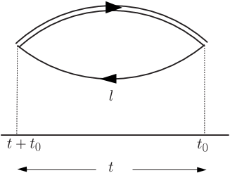
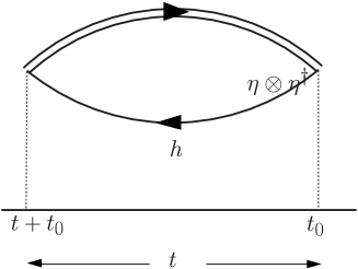
Figure 1: The diagrams for the 2-point correlation function. The left and right panels show the low-mode and high-mode contributions, respectively.

The heavy-light 3-point correlator is given by

$$C(t_{B^{*}},t_{A},t_{B}) = \frac{1}{V}\sum_{\vec{x},\vec{y},\vec{z}}\sum_{\vec{r},\vec{w}}\Big{\langle}{\rm Tr}\Big{[}S_{b}(\vec{y},t_{B};\vec{x},t_{B^{*}})\Gamma_{B^{*}_{\alpha}}\bar{Q}(\vec{x}+\vec{r},t_{B^{*}};\vec{z},t_{A})$$ (43)

$$\left.\left.\times\Gamma_{A_{\alpha}}\bar{Q}(\vec{z},t_{A};\vec{y}+\vec{w},t_{B})\tilde{\Gamma}_{B}\phi(\vec{r})\phi(\vec{w})\right]\right\rangle,$$

where $\Gamma_{B^{*}_{\alpha}}=\gamma_{\alpha}$, $\Gamma_{A_{\alpha}}=\gamma_{\alpha}$, and $\tilde{\Gamma}_{B}=-1$ ($\alpha=1,2,3$). They are decomposed into four parts:

$$C(t_{B^{*}},t_{A},t_{B}) = \Big{\langle}C_{ll}(t_{B^{*}},t_{A},t_{B})+C_{lh}(t_{B^{*}},t_{A},t_{B})$$ (44)

$$\hskip 8.5359pt+C_{hh}(t_{B^{*}},t_{A},t_{B})+C_{hl}(t_{B^{*}},t_{A},t_{B})\Big{\rangle}.$$

Here, $C_{ll}$, $C_{lh}$, $C_{hh}$, and $C_{hl}$ denote the low-low, low-high, high-high, and high-low mode correlators, respectively, which are schematically depicted in Fig. 2.

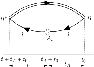
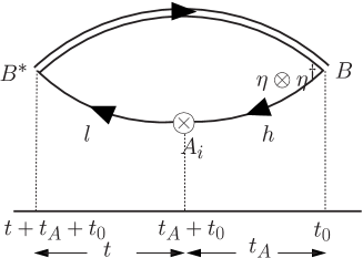
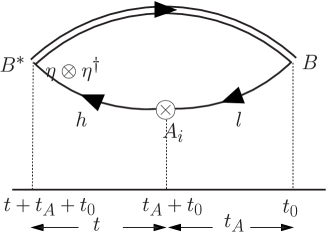
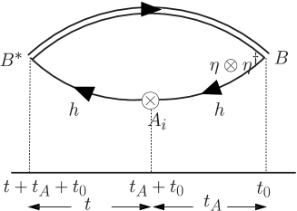
Figure 2: The diagrams for the 3-point correlation function. The top left and right panels display the lower-lower and lower-higher parts and bottom left and right panels display the higher-lower and higher-higher parts.

Explicit expressions of the 3-point functions are given in the Appendix.

As noted for the 2-point correlation functions, translationally equivalent correlators can be averaged over an appropriate number of source time slices. For the low-low part, we averaged over all the source time slices, since the numerical cost is small. For the other three parts, we explore the best solution in the following section.

6 Simulation details

Our simulations were carried out on a quenched $16^{3}\!\times 48$ lattice with the standard plaquette gauge action $\beta=6/g^{2}=6.0$. We considered 32 gauge configurations generated by the pseudo-heat-bath update algorithm, each separated by 1000 Monte Carlo sweeps, after a period of 1,000 sweeps allowed for thermalization.

In the HQET, we used the static action with HYP smeared links and the parameter value $(\alpha_{1},\alpha_{2},\alpha_{3})=(0.75,0.6,0.3)$. We used the $\cal O\it(a)$-improved Wilson fermion for the light quark with the nonperturbatively determined clover coefficient $c_{\rm SW}=1.769$ [23]. We considered three hopping parameters, $\kappa=0.1335$, 0.1340, and 0.1342. The $B$ and $B^{*}$ meson operators at both the source and sink points were smeared with the smearing function $\phi(t,\vec{r})\propto\exp(-0.45|\vec{r}|)$. This smearing function was obtained from the wavefunction given in Ref.24) by properly scaling the parameters to our lattice spacing. The low-lying eigenmodes of $Q$ were obtained with the implicitly restarted Lanczos algorithm [25], accelerated by spectral transformation with the Chebyshev polynomial of degree 80 [26]. The low-mode parts of the correlation functions can be computed with these eigenvectors. For the high-mode parts of the correlator, we obtained the quark propagator with a source vector which is given by a normalized complex $Z_{2}$ random noise and then projected into the space perpendicular to the space spanned by the low modes. Then, the time, color, and spinor dilution was applied, and all color and spinor components were summed over, while the number of the time dilution, $N_{t_{0}}$, may be kept less than the total time $N_{t}=48$. The Dirac operator was then inverted using the BiCGStab algorithm with the stopping condition $10^{-10}$. The number of eigenmodes for the low-mode averaging was chosen to be $N_{\rm ev}=100$ and the number of the random noise and the time dilution was taken to be $N_{r}=1$ and $N_{t_{0}}=4$ for our final productive run. This choice was made so as to realize good statistical accuracy of the correlators while keeping the numerical cost at a reasonable level, based on our exploratory study of the 2-point and 3-point functions by changing the parameter choices. This is explained below.

6.1 Exploratory study of the parameter choice for all-to-all propagators

In this subsection, we report the results of exploratory studies to determine the optimal parameter value for the all-to-all propagators in order to realize maximum numerical accuracy of the correlators with modest numerical cost. We found that obtaining 100 low eigenmodes is feasible, because it costs about two hours per configuration of our computational resources;  this cost is not large compared to that of the other parts of the calculation. For the correlator, the numerical cost for the all-to-all propagators for the low-mode part grows linearly in $N_{\rm ev}$ for 2-point correlators, since there is only one light quark propagator in the diagram, while for 3-point correlators it grows quadratically in $N_{\rm ev}$, because there are two light quark propagators in the diagram. Then, the numerical cost for the high-mode part grows linearly both in $N_{t_{0}}$ and $N_{r}$, because we apply the source method to compute the high-high part of the 3-point correlation functions.

In the exploratory analysis described below we studied the parameter dependence using the data with 32 configurations for both 2-point and 3-point correlators. All the studies of the 2-point correlator were carried out with $N_{r}=1$. Except for the study of the $N_{t_{0}}$ dependence, the 2-point functions were basically studied with $N_{t_{0}}=4$, while in the final production run, we used $N_{t_{0}}=48$. For the 3-point correlators, basic studies were carried out for $(N_{r},N_{t_{0}},t_{A})=(1,4,8)$ except for the study of the $(N_{r},N_{t_{0}})$ and $t_{A}$ dependences, while for the production run, the same parameter values were adopted.

6.1.1 $N_{\rm ev}$ dependence of the 2-point correlator

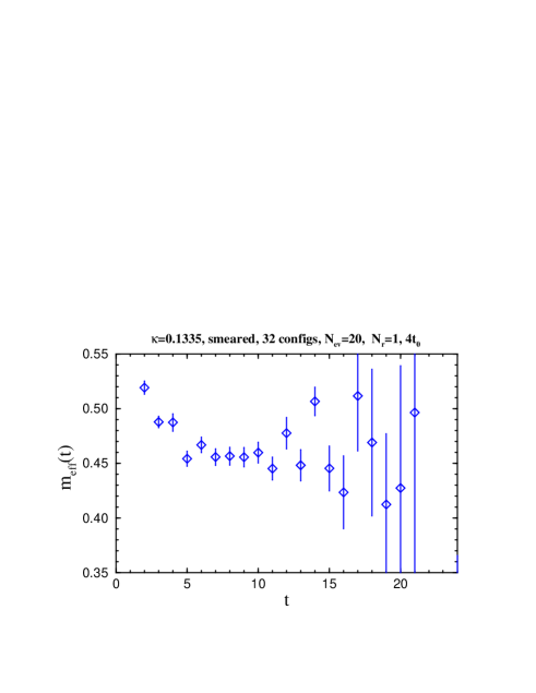
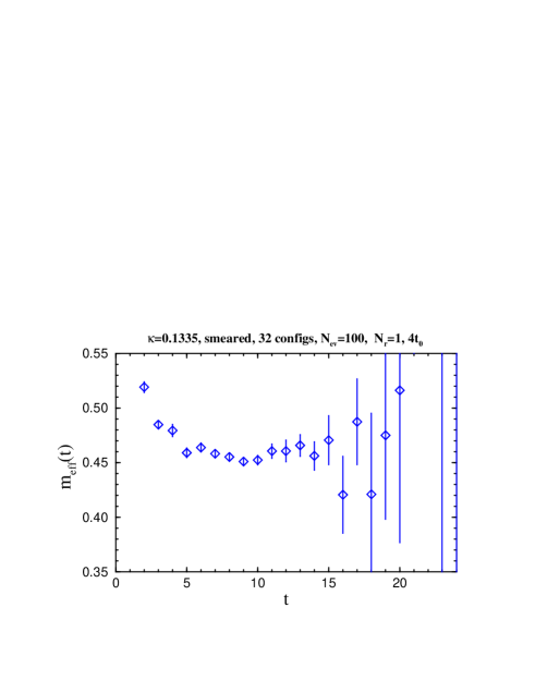
Figure 3: Plots of the effective mass of the 2-point correlators for $\kappa=0.1335$, with low mode averaging and $N_{t_{0}}=4$ and $N_{r}=1$ for high modes. The top, middle and bottom panels correspond to $N_{\rm ev}=0$, 20, and 100, respectively.

We first study the $N_{\rm ev}$ dependence of the 2-point correlators. The low-mode averaging gives the exact all-to-all propagator for the low mode part, and thus it improves the statistical accuracy of the low-mode contribution significantly. Therefore if the low-mode contribution dominates the 2-point function for the time range where the effective mass exhibits a plateau, one can expect that better accuracy can be obtained. Figure 3 plots the effective mass of the 2-point correlators for three choices of the number of low eigenmodes, $N_{\rm ev}=0,20$ and $100$, with $N_{r}=1$ for $\kappa=0.1335$. The statistical fluctuations apparently decrease as $N_{\rm ev}$ increases, and for $N_{\rm ev}=100$ we observe a clear plateau for $t\geq 7$. The situation is almost the same for $\kappa=0.1342$.

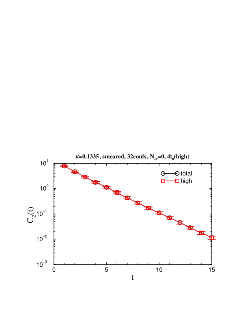
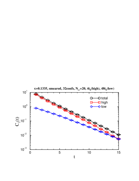
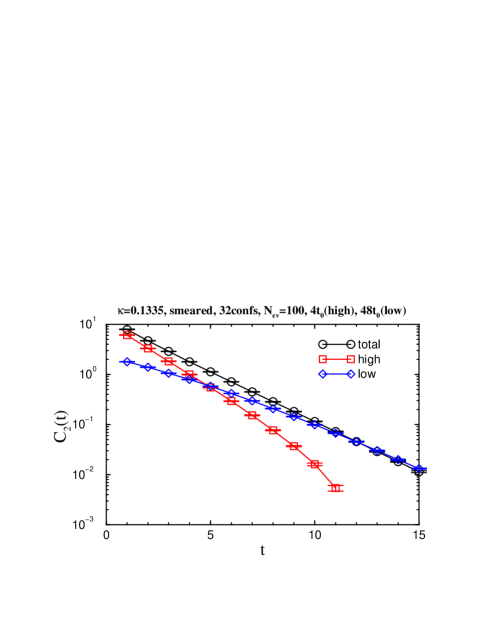
Figure 4: Low-mode and high-mode contributions to the 2-point correlators for $\kappa=0.1335$ with low-mode averaging and $N_{t_{0}}=4$ and $N_{r}=1$ for the high modes. The top, middle and bottom panels correspond to $N_{\rm ev}=0$,20, and 100, respectively.

The behavior described above can be understood as the low-mode dominance in the correlator for large $t$. Because we used the low-mode averaging, the low-mode part has the best accuracy. For the high-mode part, we only averaged over $N_{t_{0}}=4$ timeslices for source points in this particular analysis, and for this reason, maximal statistical accuracy was not obtained. Also, the high-mode part suffers from additional statistical error due to the random source for the noisy estimator. These makes the high-mode part much noisier than the low-mode part. Figure. 4 shows the low-mode and high-mode contributions to the 2-point correlators for different choices of the number of low eigenmodes, $N_{\rm ev}$. We find that for $N_{\rm ev}=100$, the low-mode contribution dominates the 2-point correlator for $t\geq 6$, where the plateau has almost been reached, while for $N_{\rm ev}=20$, low-mode dominance is obtained only for $t>15$.

Although the 100 eigenmode calculation requiring 2 hours is rather time consuming, it still worthwhile to consider larger computational times for the 3-point correlators. Carrying out the complete low-mode averaging of the 2-point correlators takes about 35 minutes per configuration. The computation for the high modes with averaging over four time slices typically takes another 35 minutes, while averaging over all 48 time slices would typically take 7 hours. This means that choosing $N_{\rm ev}=100$ and reducing the effect of the noisy high mode contribution is the optimal choice.

6.1.2 Effect of low mode averaging for the 2-point correlator

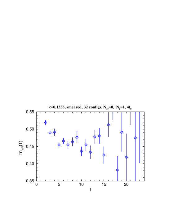
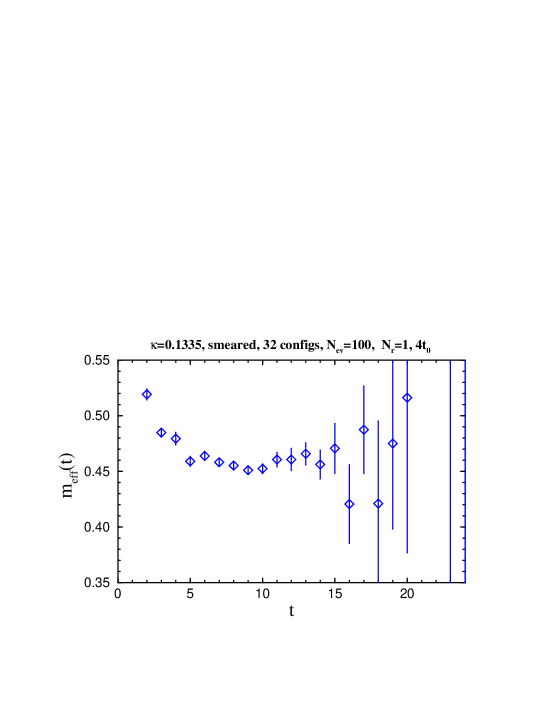
Figure 5: Plots of the effective mass of the 2-point correlators for $\kappa=0.1335$ with low mode averaging over 4 time slices (top panel) and 48 time slices (bottom panel), with $N_{r}=1$ and $N_{\rm ev}=100$.

Although it is obvious that once we have the low eigenmodes we should carry out complete low-mode averaging, it would still be interesting to see how much gain in statistical accuracy we obtain with the low-mode averaging. For this purpose, we compare the results obtained with averaging over only four source time slices and those obtained with averaging over all time slices for the low-mode part. Figure 5 presents a comparison of the effective mass plots of the 2-point correlators. There, the low-mode contributions were averaged over four equally time slices separated and over 48 timeslices. There is obviously a significant improvement in the statistics. Considering the errors for $t=$5–10 we find that increasing $N_{t_{0}}$ from 4 to 48, the statistical error is further reduced by a factor of 2–3, which is effectively equivalent to having 4-9 more statistically independent configurations. This suggests that out of the 48 time slices of 8–12 time slices are effectively statistically independent.

6.1.3 Effect of $t_{0}$ averaging for the high-mode part for the 2-point correlator

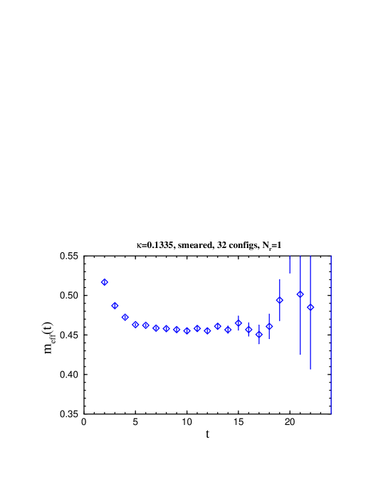
Figure 6: Plots of the effective mass of the 2-point correlators for $\kappa=0.1335$ with complete low mode averaging. The high-mode part is averaged over 4 time slices (top) and 48 time slices (bottom), with $N_{r}=1$ and $N_{\rm ev}=100$.

We also studied the effect of $t_{0}$ averaging for the high-mode contribution. In Fig. 6, we compare the data with $N_{t_{0}}=4$ and $N_{t_{0}}=48$. It is seem that we obtain a clearer plateau for the data with $N_{t_{0}}=48$. In fact, the errors for the data with $N_{t_{0}}=4$ are larger by a factor of approximately 1.5–2 than those with $N_{t_{0}}=48$ due to the reduction in the error for the high mode part, which is not a negligible contribution. This is because, even though the high-mode contribution itself is small, its error is roughly equal to that of the low- mode parts.

The data with $N_{t_{0}}=48$ in Fig. 6 also exhibits a clean plateau which starts at $t=7$, or perhaps even a smaller value. From this result, in the study of 3-point correlators reported below, we chose $t_{A}=7$ , 8, and 9.

6.1.4 $N_{r}$ dependence of the 2-point correlator

It is also possible to reduce the error by increasing $N_{r}$. However, as pointed out by the TrinLat group, increasing $N_{r}$ only reduces the error from the noisy estimator in the high mode, while increasing $N_{t_{0}}$ reduces the error from both the noisy estimator and the fluctuation of the gauge field. Since the numerical cost of computing the 2-point correlator is relatively small, we decided to use $N_{t_{0}}=48$ and $N_{r}=1$, which already gives sufficiently good results. We postpone the actual study of the $N_{r}$ dependence to a later subsection, where we study the 3-point correlators.

6.1.5 Low mode dominance in the 3-point correlator

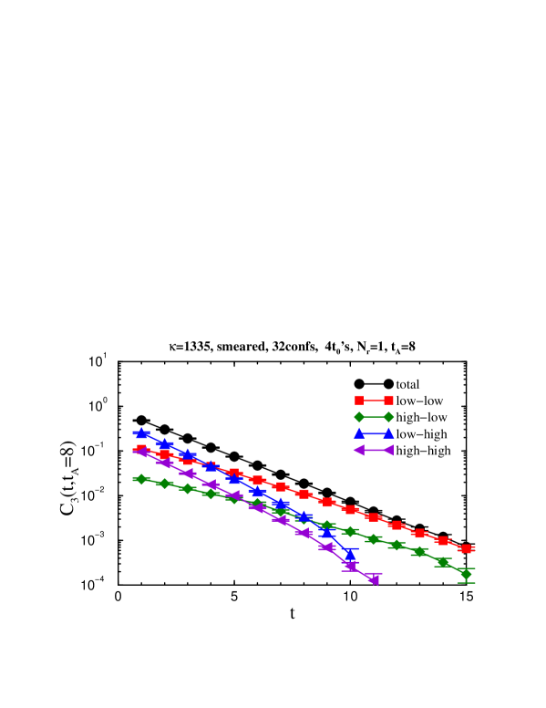
Figure 7: Contributions of the low-low, high-low, low-high and high-high parts to the total 3-point function.

Now we turn to the 3-point correlators, for which we study the contribution of low-low, high-low, low-high and high-high modes. Figure 7 shows the contribution of each mode to the 3-point correlator for $\kappa=0.1335$, $N_{\rm ev}=100$, $(N_{r},N_{t_{0}})=(1,4)$ and $t_{A}=8$. We find that for $t<9$ $(t+t_{A}<17)$ high-low and low-low are the two dominant contributions, with high-low larger for $t\leq 4$ $(t+t_{A}\leq 12)$ and low-low larger for $t\geq 5$ $(t+t_{A}\geq 13)$.

While it is true that low-mode averaging does help to reduce the error, it is also important to reduce the error for the high-low contribution by carrying out more averaging for the high-modes. This is realized in two independent ways. One is to take a larger $N_{t_{0}}$ for averaging the high-mode over the timeslices of the source points. The other is to increase $N_{r}$. In the next subsections we examine the effects of both.

6.1.6 $(N_{r},N_{t_{0}})$ dependences of the 3-point correlator

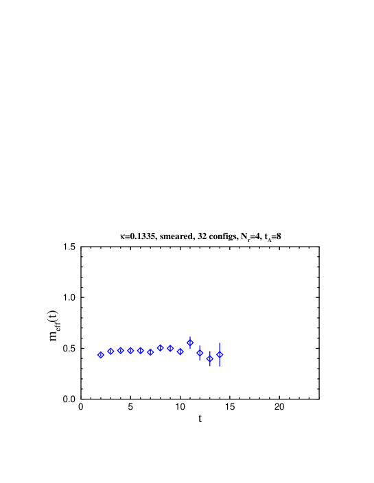
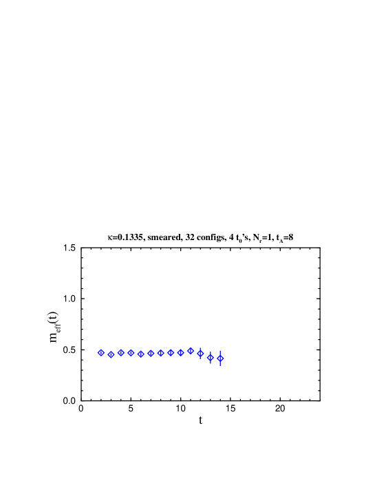
Figure 8: Plots of the effective mass of the 3-point correlators for $\kappa=0.1335$ for $(N_{r},N_{t_{0}})=(1,1)$(top), $(N_{r},N_{t_{0}})$ = (4,1) (middle) and (1,4) (bottom), with $t_{A}=8$, $N_{\rm ev}=100$.

Figure 8 plots the $(N_{r},N_{t_{0}})$ dependences of the 3-point correlator with $t_{A}=8$. We find that increasing $N_{r}$ from 1 to 4 reduces the statistical errors by a factor of approximately 0.7, while increasing $N_{t_{0}}$ from 1 to 4 reduces the statistical errors for all $t$ by a factor of approximately 0.5. Therefore, we find that for given computational resources, increasing $N_{t_{0}}$ is more efficient than increasing $N_{r}$. This is as expected, since increasing $N_{t_{0}}$ reduces both the error from the gauge fluctuation and the error from the noisy estimator, while increasing $N_{r}$ reduces only the latter.

6.1.7 $t_{A}$ dependence

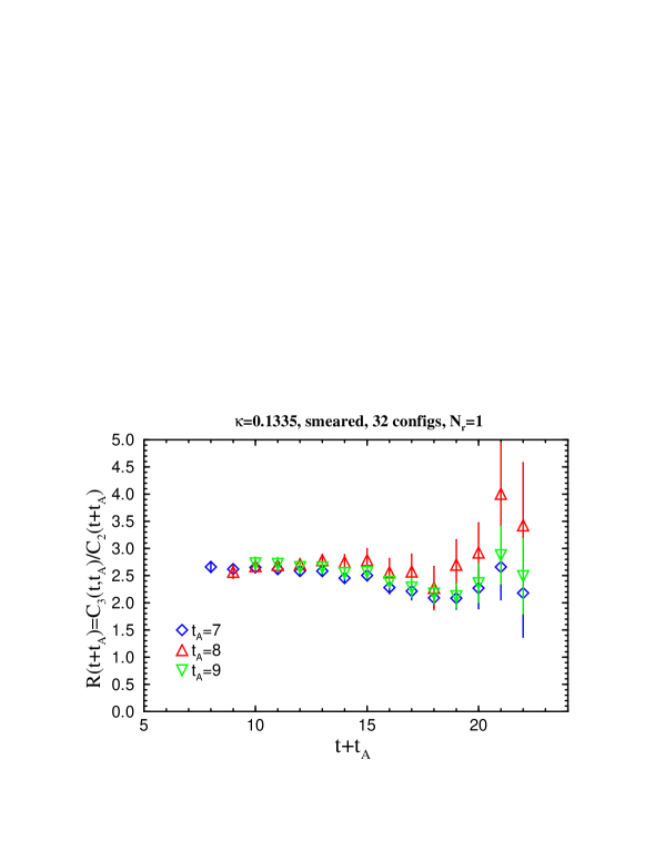
Figure 9: $t_{A}$ dependence of the 3-point/2-point correlator ratio for $\kappa=0.1335$ with $(N_{r},N_{t_{0}})=(1,1)$ and $N_{\rm ev}=100$.

Figure 9 plots the time dependence of the 3-point/2-point ratio $R(t,t_{A})$ for $t_{A}=7,8$ and $9$. The results for $t_{A}=7,8$ and $9$ are consistent. The result of the data fit for $t_{A}=9$ is relatively poor and has large statistical error, while those for $t_{A}=7$ and $8$ do not differ in precision. From this study, we conclude that $t_{A}=8$ is a reasonable choice for the productive run. We also find that the best fitting range of $R(t,t_{A})$ is $t+t_{A}=12-16(t=4-8)$ .

7 Results

In this section, we present the results from our productive run for 32 cofingurations on $16^{3}\times 48$ lattices with $\beta=6.0$ using the $O(a)$-improved Wilson fermion with $c_{\rm SW}=1.769$. We chose three values of the hopping parameters, $\kappa=0.1335$, 0.1340, and 0.1342. For the all-to-all propagators, our choices of the parameters were

$$N_{\rm ev}=100,\ N_{t_{0}}=48,\ N_{r}=1$$ (45)

for 2-point correlator, and

$$N_{\rm ev}=100,\ N_{t_{0}}=4,\ N_{r}=1,\ t_{A}=8$$ (46)

for 3-point correlator.

7.1 2-point correlators

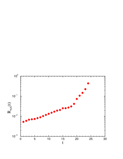
Figure 10: The ratio $R_{NS}$ for the 2-point correlation function with 32 configurations for $\kappa=0.1335$.

Figure 10 displays the noise-to-signal ratio $R_{NS}=\Delta C_{2}(t)/C_{2}(t)$ for the 2-point function. As shown in this figure the noise-to-signal ratio remains roughly in the range 1–3 % for the time range 1–2 fm.

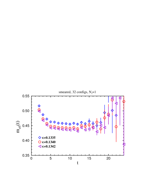
Figure 11: Plots of the effective mass of the 2-point function for $\kappa=0.1335$, 01340, and 0.1342, with $(N_{r},N_{t_{0}})=(1,48)$. We observe a clear plateau for $t\in[7,11]$

In this subsection we present our results for the 2-point correlators. Figure 11 presents effective mass plots of the 2-point functions for $\kappa=0.1335$, 0.1340, and 0.1342. Fitting the 2-point function with the fit range $t=\left[7,11\right]$, we obtain the binding energy of the heavy-light meson with 0.2 % accuracy as shown in Fig. 12. The square in Fig. 12 represents the result of the Alpha collaboration [6] for the same value $\beta=6.0$ on a $16^{3}\times 32$ lattice with the Schrödinger functional boundary conditions using on the order of a few hundred configurations. Although a simple comparison may not be meaningful, because of the different the kinematical setups used (for example, the volume, boundary conditions and operators), it is nevertheless noteworthy that the all-to-all propagators yields much better precision with a much smaller number of configurations, $N_{\rm conf}=32$. Extrapolating linearly in $(am_{\pi})^{2}$, we obtain

$$aE=0.408\pm 0.002,$$ (47)

i.e., 0.5% accuracy in the chiral limit.

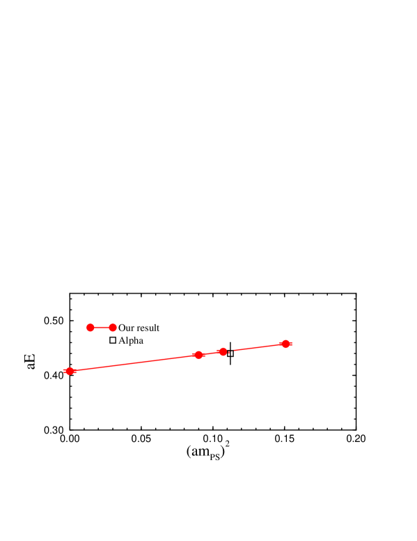
Figure 12: Binding energies from 2-point correlators. The solid circles represent our data for $\kappa=0.1335$, 0.1340, and 0.1342 with 32 configurations. The square represents the result from the Alpha collaboration with a few hundred configurations.

7.2 3-point correlators

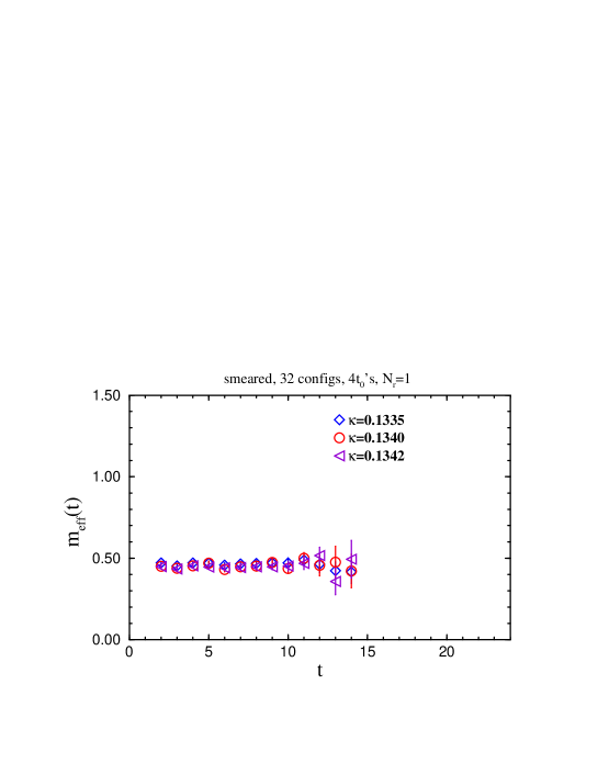
Figure 13: Plots of the effective mass of the 3-point correlation function for $\kappa=0.1335$, 0.1340, and 0.1342 with 4 $t_{0}$ sources.

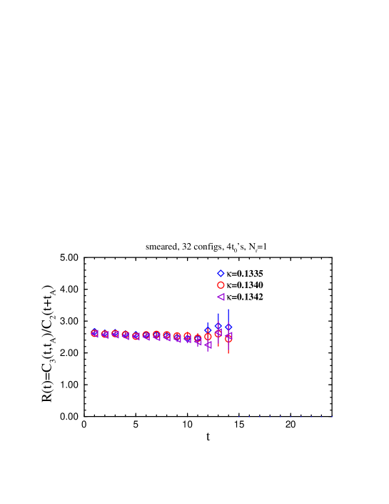
Figure 14: 3-point/2-point correlator ratio $R(t,t_{A})$ for $\kappa=0.1335$, 0.1340, and 0.1342 with 4 $t_{0}$ sources. We observe a clear plateau for $t\in[5,9]$.

Figure 13 represents plots of the effective mass of the 3-point correlators. We find that the plateau is reached for $t\geq 4$. Figure 14 displays the 3-point/2-point correlator ratios. Applying constant fits of this ratio with fitting range $t=[5,9]$, we obtain

$$R(t,t_{A})=\frac{C_{3}(t,t_{A})}{C_{2}(t+t_{A})}=2.56(5)\mbox{ for $\kappa=0.1335$},$$ (48)

$$R(t,t_{A})=\frac{C_{3}(t,t_{A})}{C_{2}(t+t_{A})}=2.55(5)\mbox{ for $\kappa=0.1340$},$$ (49)

$$R(t,t_{A})=\frac{C_{3}(t,t_{A})}{C_{2}(t+t_{A})}=2.50(4)\mbox{ for $\kappa=0.1342$},$$ (50)

where each result has 2% accuracy. The bare lattice operator for the light-light axial vector current should be renormalized as

$$A_{i} = 2\kappa Z_{A}(1+b_{A}m_{q})(A_{i}^{\rm lat}+c_{A}\partial_{i}P).$$ (51)

The second term here does not contribute after summing over all spatial positions. The quantity $Z_{A}$ has been determined nonperturbatively by the Alpha collaboration. For $\beta=6.0$, they obtained $Z_{A}=0.79$. The quantitly $b_{A}$ was also obtained by combining the results of $b_{V}$ from the Alpha collaboration [27] and $b_{A}-b_{V}$ from Battacharya et al.  [28] for $\beta=6.0$. Using the above formula, the $B^{*}B\pi$ coupling can be obtained as

$$\hat{g}_{\infty}=2\kappa Z_{A}(1+b_{A}m_{q})R.$$ (52)

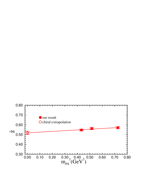
Figure 15: $\hat{g}_{\infty}$ for $\kappa=0.1335$, 0.1340, and 0.1342, together with the result in the chiral limit obtained by linear extrapolation in $(am_{\pi})^{2}$.

Figure 15 displays our results the $\hat{g}_{\infty}$ as a function of $(am_{\pi})^{2}$. Taking the chiral limit by extrapolating linearly in $(am_{\pi})^{2}$, we obtain $\hat{g}_{\infty}$ in the chiral limit as

$$\hat{g}_{\infty}=0.517\pm 0.016, \beta=6.0$$   (for ) (53)

with 3% statistical error. This result can be compared with the result on $16^{3}\times 32$ lattices for $\beta=6.0$ using the $O(a)$-improved Wilson fermion with $c_{\rm SW}=1.769$ by Abada et al [17]. Their result in the chiral limit is $\hat{g}_{\infty}=0.45(4)$, which is consistent with ours within 2$\sigma$. We note that their results for finite quark masses have 4–6% statistical errors giving 9% accuracy in the chiral limit with on the order of 100 configurations, whereas ours have 2% statistical error for finite quark masses giving 3% accuracy in the chiral limit with 32 configurations. It is thus seen that are obtain a significant improvement in statistical accuracy using the all-to-all propagators.

8 Conclusions

In this paper, we have studied the feasibility of the all-to-all propagator method for precise computation of the $B^{*}B\pi$ coupling, $\hat{g}_{\infty}$. Determining 100 eigenmodes, we find that the low-modes dominate the correlators, and therefore the low-mode averaging in the all-to-all propagator reduces the noise significantly.

For reference we, list the numerical cost estimate using 1 CPU on our vector supercomputer in Table 2.

Table 2: Computational cost per configuration for 2-point and 3-point correlators for $\kappa=0.1335$.

2-point correlator
$N_{\rm ev}$	$N_{t_{0}}$	low	high	total
0	4	-	30 min.	30 min
20	4	7 min.	35 min.	40 min
100	4	35 min.	35 min.	70 min
100	48	35 min.	7 h 25 min	8 h
3-point correlator
$N_{\rm ev}$	$N_{t_{0}}$	low-low	low-high, high-low, high-high	total
100	4	40 min.	$\sim$ 32 h	$\sim$ 33 h

For 2-point heavy-light meson correlators in quenched QCD, 8 hours are required per configuration using the all-to-all propagator with $N_{\rm ev}=100$ and $(N_{r},N_{t_{0}})=(1,48)$, while this time becomes 10 hours if the time for the eigenmode calculation is included. If the equivalent computational cost were used for the ordinary method with a single source timeslice, one would have to compute correlators with 64–80 times more configurations, which could reduce the error by a factor of 8–9. On the other hand, the errors of the 2-point correlator for 32 configuration are a factor of 0.08–0.10 smaller than those obtained with the ordinary method. Therefore, there is a marginal gain with the all-to-all propagator. We presume that the situation would be similar for 3-point correlators, although we have not made a comparison of the results obtained using all-to-all propagators and those obtained with the ordinary method.

However, the essential aim of this study is not to show that we have a marginal gain with the all-to-all propagator in quenched QCD. What is important is that our result in quenched QCD suggests that there is a significant gain in unquenched QCD, in which case generating configurations is much more costly than the measurements. Also, the fact that only 32 independent gauge configurations are sufficient for obtaining very precise results with a few percent accuracy is encouraging.

Appendix

In this appendix we give the definitions of the low-low, low-high, high-high, and high-low mode correlators, $C_{ll}$, $C_{lh}$, $C_{hh}$, and $C_{hl}$, where the first (second) index of $C_{q_{1}q_{2}}$ specifies the quark propagator from $t_{A}$ to $t_{B^{*}}$ (from $t_{B}$ to $t_{A}$). The low-low contribution to the 3-pt functions is given by

$$C_{ll}(t_{B^{*}},t_{A},t_{B}) = \frac{1}{V}\sum_{i,j=1}^{N_{\rm ev}}\frac{1}{\lambda_{i}\lambda_{j}}\sum_{\vec{x},\vec{y},\vec{z}}\sum_{\vec{r},\vec{w}}{\rm Tr}\left\{\gamma_{5}S_{b}^{\dagger}(\vec{x},t_{B^{*}};t_{B})\delta(\vec{y}-\vec{x})\gamma_{5}\Gamma_{B^{*}_{\alpha}}\right. \cdot$$ (A54)

$$\times\,\left[v^{(i)}(\vec{x}+\vec{r},t_{B^{*}})\otimes v^{(i){\dagger}}(\vec{z},t_{A_{i}})\right]\Gamma_{A_{\alpha}}$$

$$\left.\times\,\left[v^{(j)}(\vec{z},t_{A_{i}})\otimes v^{(j){\dagger}}(\vec{y}+\vec{w},t_{B})\right]\tilde{\Gamma}_{B}\phi^{\prime}(\vec{r})\phi(\vec{w})\right\}$$

$$= \frac{1}{V}\sum_{i,v}^{N_{\rm ev}}\frac{1}{\lambda_{i}\lambda_{j}}\left\{B^{ij}_{\alpha}(t_{B^{*}},t_{B})A^{ij}_{\alpha}(t_{A})\right\}, \cdot$$ (A55)

where $\alpha=1,2,3$ and

$$A^{ij}_{\alpha}(t_{A}) = \sum_{\vec{z}}v^{(i){\dagger}}(\vec{z},t_{A})\Gamma_{A_{\alpha}}v^{(j)}(\vec{z},t_{A}), \cdot$$ (A56)

$$B^{ij}_{\alpha}(t_{B^{*}},t_{B}) = \sum_{\vec{x}}v_{\phi}^{(j){\dagger}}(\vec{x},t_{B})\Gamma^{\prime}_{B}S_{b}^{{\dagger}}(\vec{x},t_{B^{*}};t_{B})\Gamma^{\prime}_{B_{\alpha}^{*}}v_{\phi^{\prime}}^{(i)}(\vec{x},t_{B^{*}}), \cdot$$ (A57)

with $\Gamma_{A\alpha}=\gamma_{\alpha}$, $\Gamma^{\prime}_{B}=\tilde{\Gamma}_{B}\gamma_{5}=-\gamma_{5}$, and $\Gamma^{\prime}_{B_{\alpha}^{*}}=\gamma_{5}\Gamma_{B_{\alpha}^{*}}=\gamma_{5}\gamma_{\alpha}$.

The low-high contribution to the 3-pt functions are given by

$$C_{lh}(t_{B^{*}},t_{A},t_{B}) = \frac{1}{V}\sum_{\vec{x},\vec{y},\vec{z}}\sum_{\vec{r},\vec{w}}{\rm Tr}\Big{\{}S_{b}(\vec{y},t_{B};\vec{x},t_{B^{*}})\Gamma_{B^{*}_{\alpha}}\bar{Q}_{0}(\vec{x}+\vec{w},t_{B^{*}};\vec{z},t_{A})$$

$$\times\,\Gamma_{A_{\alpha}}\bar{Q}_{1}(\vec{z},t_{A};\vec{y}+\vec{w},t_{B})\tilde{\Gamma}_{B}\phi(\vec{r})\phi(\vec{w})\Big{\}}$$

$$= \frac{1}{V}\frac{1}{N_{r}}\sum_{i=1}^{N_{\rm ev}}\frac{1}{\lambda_{i}}\sum_{r,j}\sum_{\vec{x},\vec{y},\vec{z}}\sum_{\vec{r},\vec{w}}{\rm Tr}\Big{\{}\gamma_{5}S_{b}^{\dagger}(\vec{x},t_{B^{*}};t_{B})\delta(\vec{y}-\vec{x})\gamma_{5}\Gamma_{B^{*}_{\alpha}}$$

$$\times\left[v^{(i)}(\vec{x}+\vec{r},t_{B^{*}})\otimes v^{(i){\dagger}}(\vec{z},t_{A})\right]\Gamma_{A_{\alpha}}$$

$$\times\left[\psi_{[r]}^{\prime(j)}(\vec{z},t_{A_{i}})\otimes\eta_{[r]}^{(j){\dagger}}(\vec{y}+\vec{w},t_{B})\right]\tilde{\Gamma}_{B}\phi(\vec{r})\phi(\vec{w})\Big{\}}$$

$$= \frac{1}{V}\frac{1}{N_{r}}\sum_{i=1}^{N_{\rm ev}}\frac{1}{\lambda_{i}}\sum_{r,j}B^{ij}_{[r]\alpha}(t_{B^{*}},t_{B})\cdot A^{ij}_{[r]\alpha}(t_{A}), \cdot$$ (A59)

where

$$A^{ij}_{\alpha}(t_{A}) = \sum_{\vec{z}}v^{(i){\dagger}}(\vec{z},t_{A})\Gamma_{A_{\alpha}}\psi^{(j)}_{[r]}(\vec{z},t_{A}), \cdot$$ (A60)

$$B^{ij}_{\alpha}(t_{B^{*}},t_{B}) = \sum_{\vec{x}}\eta_{[r]\phi}^{(j){\dagger}}(\vec{x},t_{B})\Gamma^{\prime}_{B}S_{b}^{{\dagger}}(\vec{x},t_{B^{*}};t_{B})\Gamma^{\prime}_{B_{\alpha}^{*}}v_{\phi}^{(i)}(\vec{x},t_{B^{*}}). \cdot$$ (A61)

While we repeatedly use the symbols $A^{ij}_{\alpha}(t_{A})$ and $B^{ij}_{\alpha}(t_{B^{*}},t_{B})$, we anticipate there will be no confusion, since they are valid only in the expression just before they are defined.

In the case of $C_{hl}$, we set the source of the noisy estimator to $t_{B^{*}}$. Since $Q_{1}$ is hermitian, we have

$$\bar{Q}_{1}(x,z)=\bar{Q}_{1}(z,x)^{\dagger}=\frac{1}{N_{r}}\sum_{r,i}\left[\psi^{j}_{[r]}(z)\otimes\eta^{j{\dagger}}_{[r]}(x)\right]^{\dagger}=\frac{1}{N_{r}}\sum_{r,i}\left[\eta^{j}_{[r]}(x)\otimes\psi^{j{\dagger}}_{[r]}(z)\right]. \cdot$$ (A62)

This leads to

$$C_{hl}(t_{B^{*}},t_{A},t_{B}) = \frac{1}{V}\sum_{\vec{x},\vec{y},\vec{z}}\sum_{\vec{r},\vec{w}}{\rm Tr}\Big{\{}S_{b}(\vec{y},t_{B};\vec{x},t_{B^{*}})\Gamma_{B^{*}_{\alpha}}\bar{Q}_{1}(\vec{x}+\vec{w},t_{B^{*}};\vec{z},t_{A})$$

$$\times\,\Gamma_{A_{\alpha}}\bar{Q}_{0}(\vec{z},t_{A};\vec{y}+\vec{w},t_{B})\tilde{\Gamma}_{B}\phi(\vec{r})\phi(\vec{w})\Big{\}}$$

$$= \frac{1}{V}\frac{1}{N_{r}}\sum_{j=1}^{N_{\rm ev}}\frac{1}{\lambda_{j}}\sum_{r,i}\sum_{\vec{x},\vec{y},\vec{z}}\sum_{\vec{r},\vec{w}}{\rm Tr}\Big{\{}S_{b}(\vec{x},t_{B};t_{B^{*}})\delta(\vec{y}-\vec{x})\Gamma_{B^{*}_{\alpha}}$$

$$\times\,\left[\eta^{(i)}_{[r]}(\vec{x}+\vec{r},t_{B^{*}})\otimes\psi^{(i){\dagger}}_{[r]}(\vec{z},t_{A})\right]\Gamma_{A_{\alpha}}$$

$$\times\,\left[v^{(j)}(\vec{z},t_{A_{i}})\otimes v^{(j){\dagger}}(\vec{y}+\vec{w},t_{B})\right]\tilde{\Gamma}_{B}\phi(\vec{r})\phi(\vec{w})\Big{\}},\hskip 14.22636pt$$

$$= \frac{1}{V}\frac{1}{N_{r}}\sum_{i=1}^{N_{\rm ev}}\frac{1}{\lambda_{i}}\sum_{r,j}B^{ij}_{[r]\alpha}(t_{B^{*}},t_{B})\cdot A^{ij}_{[r]\alpha}(t_{A}), \cdot$$ (A64)

where

$$A^{ij}_{\alpha}(t_{A}) = \sum_{\vec{z}}\psi^{(i){\dagger}}_{[r]}(\vec{z},t_{A})\Gamma_{A_{\alpha}}v^{(j)}(\vec{z},t_{A}), \cdot$$ (A65)

$$B^{ij}_{\alpha}(t_{B^{*}},t_{B}) = \sum_{\vec{x}}v_{\phi}^{(j){\dagger}}(\vec{x},t_{B})\tilde{\Gamma}_{B}S_{b}(\vec{x},t_{B};t_{B^{*}})\Gamma_{B_{\alpha}^{*}}\eta_{[r]\phi}^{(i)}(\vec{x},t_{B^{*}}). \cdot$$ (A66)

Recall that $\Gamma_{B^{*}_{\alpha}}=\gamma_{\alpha}$, $\Gamma_{A_{\alpha}}=\gamma_{\alpha}$, and $\tilde{\Gamma}_{B}=-1$ ($\alpha=1,2,3$).

The high-high part, $C_{hh}^{(1)}$, is evaluated using the noisy estimator with a source vector put on the time slice $t_{B}$:

$$C_{hh}(t_{B^{*}},t_{A},t_{B}) = \frac{1}{V}\sum_{\vec{x},\vec{y},\vec{z}}\sum_{\vec{r},\vec{w}}{\rm Tr}\Big{\{}S_{b}(\vec{y},t_{B};\vec{x},t_{B^{*}})\Gamma_{B^{*}_{\alpha}}\bar{Q}_{1}(\vec{x}+\vec{w},t_{B^{*}};\vec{z},t_{A}) \cdot$$ (A68)

$$\times\,\Gamma_{A_{\alpha}}\bar{Q}_{1}(\vec{z},t_{A};\vec{y}+\vec{w},t_{B})\tilde{\Gamma}_{B}\phi(\vec{r})\phi(\vec{w})\Big{\}}$$

$$= \frac{1}{V}\frac{1}{N_{r}}\sum_{r,i}\sum_{\vec{x},\vec{y},\vec{z}}\sum_{\vec{r},\vec{w}}{\rm Tr}\Big{\{}S_{b}(\vec{y},t_{B};\vec{x},t_{B^{*}})\Gamma_{B^{*}_{\alpha}}\bar{Q}_{1}(\vec{x}+\vec{w},t_{B^{*}};\vec{z},t_{A})$$

$$\times\,\Gamma_{A_{\alpha}}\left[\psi^{(i)}_{[r]}(\vec{z},t_{A})\otimes\eta^{(i){\dagger}}_{[r]}(\vec{y}+\vec{w},t_{B})\right]\tilde{\Gamma}_{B}\phi(\vec{r})\phi(\vec{w}).$$

Using the source method,

$$\Psi_{[r]\alpha}^{(i)}(\vec{x},t_{B^{*}};t_{A}) = \sum_{\vec{z}}\bar{Q}_{1}(\vec{x},t_{B^{*}};\vec{z},t_{A})\Gamma_{A_{\alpha}}\psi^{(i)}_{[r]}(\vec{z},t_{A}) \cdot$$ (A69)

$$= \sum_{\vec{z}}D^{-1}(\vec{x},t_{B^{*}};\vec{z},t_{A})\gamma_{5}P_{1}\Gamma_{A_{\alpha}}\psi^{(i)}_{[r]}(\vec{z},t_{A})$$

can be obtained by solving the linear equation $D\Psi=b$, with the source vector $b=\gamma_{5}P_{1}\Gamma_{A_{\alpha}}\psi^{(i)}_{[r]}(\vec{z},t_{A})$. Then $C_{hh}$ is obtained as

$$C_{hh}(t_{B^{*}},t_{A},t_{B})=\frac{1}{V}\frac{1}{N_{r}}\sum_{r,i}\sum_{\vec{x}}\eta^{(i){\dagger}}_{[r]\phi}(\vec{x},t_{B})\tilde{\Gamma}_{B}S_{b}(\vec{x},t_{B};t_{B^{*}})\Gamma_{B^{*}_{\alpha}}\Psi_{[r]\alpha,\phi}^{(i)}(\vec{x},t_{B^{*}};t_{A}). \cdot$$ (A70)

We must solve $3\times N_{t_{A}}$ linear equations per noise vector, where $N_{t_{A}}$ is the number of sampled time slices $t_{A}$.

References

- [1] BaBar Collaboration, talk at Joint Pacific Region Particle Physics, Hawaii, Oct. 29-Nov. 03 2006.
- [2] J. Heitger and R. Sommer (ALPHA Collaboration), J. High Energy Phys. 02 (2004), 022; hep-lat/0310035.
- [3] G. M. de Divitiis, M. Guagnelli, F. Palombi, R. Petronzio and N. Tantalo, Nucl. Phys. B 672 (2003), 372 ; hep-lat/0307005.
- [4] G. M. de Divitiis, M. Guagnelli, R. Petronzio, N. Tantalo and F. Palombi, Nucl. Phys. B 675 (2003), 309; hep-lat/0305018.
- [5] D. Guazzini, R. Sommer and N. Tantalo, PoS LAT2006 (2006), 084; hep-lat/0609065.
- [6] M. Della Morte, S. Durr, J. Heitger, H. Molke, J. Rolf, A. Shindler and R. Sommer (ALPHA Collaboration), Phys. Lett. B 581 (2004), 93 [Erratum-ibid. B 612 (2005), 313]; hep-lat/0307021.
- [7] A. Hasenfratz and F. Knechtli, Phys. Rev. D 64 (2001), 034504; hep-lat/0103029.
- [8] J. Foley, K. Jimmy Juge, A. O’Cais, M. Peardon, S. M. Ryan and J. I. Skullerud, Comput. Phys. Commun. 172 (2005), 145; hep-lat/0505023.
- [9] K. C. Bowler et al. (UKQCD Collaboration), Phys. Lett. B 486 (2000), 111; hep-lat/9911011.
- [10] A. Abada et al., D. Becirevic, P. Boucaud, J. P. Leroy, V. Lubicz and F. Mescia, QCD,” Nucl. Phys. B 619 (2001), 565; hep-lat/0011065.
- [11] A. X. El-Khadra et al., A. S. Kronfeld, P. B. Mackenzie, S. M. Ryan and J. N. Simone, QCD,” Phys. Rev. D 64 (2001), 014502; hep-ph/0101023.
- [12] S. Aoki et al. (JLQCD Collaboration), Phys. Rev. D 64 (2001), 114505; hep-lat/0106024.
- [13] E. Gulez, A. Gray, M. Wingate, C. T. H. Davies, G. P. Lepage and J. Shigemitsu, Phys. Rev. D 73 (2006), 074502; hep-lat/0601021.
- [14] M. Okamoto et al. (Fermilab Lattice Collaboration), hep-lat/0409116.
- [15] J. Shigemitsu et al. (HPQCD Collaboration), hep-lat/0408019.
- [16] G. M. de Divitiis, L. Del Debbio, M. Di Pierro, J. M. Flynn, C. Michael and J. Peisa (UKQCD Collaboration), J. High Energy Phys. 10, 010 (1998); hep-lat/9807032.
- [17] A. Abada, D. Becirevic, Ph. Boucaud, G. Herdoiza, J. P. Leroy, A. Le Yaouanc and O. Pene, J. High Energy Phys. 02 (2004), 016; hep-lat/0310050.
- [18] D. Becirevic, B. Blossier, Ph. Boucaud, J. P. Leroy, A. LeYaouanc and O. Pene, PoS LAT2005 (2006), 212; hep-lat/0510017.
- [19] C. G. Boyd and B. Grinstein, Nucl. Phys. B 442 (1995), 205; hep-ph/9402340.
- [20] T. A. DeGrand and U. M. Heller [MILC collaboration], Phys. Rev. D 65 (2002), 114501; hep-lat/0202001.
- [21] L. Giusti, P. Hernandez, M. Laine, P. Weisz and H. Wittig, J. High Energy Phys. 04 (2004), 013; hep-lat/0402002.
- [22] L. Giusti and S. Necco, PoS LAT2005 (2006), 132; hep-lat/0510011.
- [23] M. Luscher, S. Sint, R. Sommer, P. Weisz and U. Wolff, Nucl. Phys. B 491 (1997), 323; hep-lat/9609035.
- [24] A. Duncan, E. Eichten, J. Flynn, B. Hill, G. Hockney and H. Thacker, Phys. Rev. D 51 (1995), 5101; hep-lat/9407025.
- [25] D. C. Sorensen, SIAM J. Matrix Anl. Appl. 13 (1992), 357.
- [26] H. Neff, N. Eicker, T. Lippert, J. W. Negele and K. Schilling, Phys. Rev. D 64 (2001), 114509; hep-lat/0106016.
- [27] S. Sint and P. Weisz, Nucl. Phys. B 502 (1997), 251; hep-lat/9704001.
- [28] T. Bhattacharya, R. Gupta, W. J. Lee and S. R. Sharpe, Phys. Rev. D 63 (2001), 074505; hep-lat/0009038.