Generalised parton distributions of the pion in partially-quenched chiral perturbation theory

Abstract

We consider the pion matrix elements of the isoscalar and isovector combinations of the vector and tensor twist-two operators that determine the moments of the various pion generalised parton distributions. Our analysis is performed using partially-quenched chiral perturbation theory. We work in the SU(2) and SU(4$|$2) theories and present our results at infinite volume and also at finite volume where some subtleties arise. These results are useful for extrapolations of lattice calculations of these matrix elements at small momentum transfer to the physical regime.

I Introduction

Generalised parton distributions (GPDs) Müller et al. (1994); Ji (1997a, b); Radyushkin (1997) provide a uniquely detailed view of the structure of hadrons, unifying the information encoded in form-factors and parton distributions, and supplementing both. Ongoing experiments at DESY Airapetian et al. (2001); Adloff et al. (2001); Chekanov et al. (2003) and Jefferson Lab Stepanyan et al. (2001) (see Refs. Diehl (2003); Belitsky and Radyushkin (2005) for recent reviews) seek to learn about these fundamental quantities in deeply-virtual Compton scattering (DVCS) and related processes. Aspects of GPDs are also being investigated in QCD and phenomenological models. Since GPDs encode long distance hadronic structure, QCD analyses of them are necessarily based on non-perturbative methods such as lattice QCD. These examinations are complementary to the experimental efforts in that different facets of the GPDs can be accessed. Most experimental efforts are focused on the proton and either measure the GPDs at constrained kinematics (through polarisation observables) or measure integrals of the GPDs (through DVCS cross-sections). Lattice QCD analyses are based on the operator product expansion and lead to information on the lowest few Mellin moments of the GPDs which correspond to non-forward matrix elements of twist-two operators. Again most studies focus on the proton Hägler et al. (2003); Göckeler et al. (2004); Hägler et al. (2004); Göckeler et al. (2005), but the GPDs of other hadrons are equally accessible in the lattice approach (unlike in experiment). In particular, recent studies by the QCDSF collaboration Brömmel et al. (2005) have investigated the GPDs of the pion.

Here we investigate the vector and tensor GPDs of the pions from the point of view of chiral perturbation theory applied to lattice QCD, studying the quark mass and lattice volume dependence of the meson matrix elements of twist-two operators. Related studies of the vector GPD pion matrix elements have been presented in Ref. Arndt and Savage (2002); Chen and Ji (2001); Kivel and Polyakov (2002); Detmold et al. (2003); Chen and Stewart (2004); Diehl et al. (2005), however we extend those results to partially-quenched chiral perturbation theory (appropriate for lattice calculations with differing sea- and valence- quark masses). We also consider the tensor twist-two operators (also treated recently in Ref. Diehl et al. (2006a)) and include the effects of the finite volume to which lattice simulations are necessarily restricted (the Lorentz non-invariance of the lattice boundary conditions introduces some novel issues in the resulting extrapolation that we highlight). The finite volume calculations in partially-quenched chiral perturbation theory are particularly relevant to the ongoing lattice calculations reported in Ref. Brömmel et al. (2005) (see Best et al. (1997) for earlier work in the forward limit).

In the following section we provide our notation and conventions for the pion GPDs and twist-two matrix elements. In Section III we turn to the effective field theory description of these objects before presenting our infinite volume results in Section IV, their finite volume analogues in Section V, and a concluding discussion in Section VI. Various aspects of the finite volume forms are relegated to the Appendix.

II Generalised parton distribution of the pion

II.1 Pion GPDs

The generalised parton distributions of the pions (here we restrict our discussion to SU(2)) are defined by matrix elements of light-cone separated bi-local currents. Specifically, the vector GPDs $H^{A}$, and the tensor GPDs, $E_{T}^{A}$, are given by

$$\langle\pi^{i}(p^{\prime})|\,\overline{\psi}\left(-\frac{z}{2}n\right)\tau^{A}\gamma\cdot u\psi\left(\frac{z}{2}n\right)|\pi^{j}(p)\rangle = \int_{-1}^{1}dye^{-iyzu\cdot\bar{P}}H^{A}(y,\xi,t)u\cdot\bar{P}\text{tr}\left[\ \!\!\tau^{i}\tau^{A}\tau^{j}\right]\ ,$$ (1)

and

$$\langle\pi^{i}(p^{\prime})|\,\overline{\psi}\left(-\frac{z}{2}n\right)\tau^{A}i\,\sigma^{\mu\nu}u_{\mu}r_{\nu}\psi\left(\frac{z}{2}n\right)|\pi^{j}(p)\rangle = \int_{-1}^{1}dye^{-iyzu\cdot\bar{P}}E_{T}^{A}(y,\xi,t)u\cdot\bar{P}r\cdot\Delta\text{tr}\left[\ \!\!\tau^{i}\tau^{A}\tau^{j}\right]\ ,$$ (2)

respectively (for simplicity, we have suppressed the gauge links that render these matrix elements gauge invariant). Here the average four momentum of the incoming and outgoing pion states is $\overline{P}=\frac{1}{2}(p+p^{\prime})$ and the momentum transfer is $\Delta=p^{\prime}-p$, $u$ is a light-like vector ($u^{2}=0$) and $r$ is transverse ($r\cdot u=r\cdot\overline{P}=0$). The GPDs are functions of the three variables $y$, $\xi=-\frac{u\cdot\Delta}{2u\cdot\overline{P}}$ and $t=\Delta^{2}$. Finally, $\tau_{A}=(\bf{1},\tau_{A})$ for QCD.

II.2 Twist-two operators

As is evident from the forms of the GPDs, there are two towers of local twist-two quark operators that have non-vanishing pion matrix elements. These are given by

$${\cal O}^{(n)}_{A}\equiv u_{\mu_{0}}\ldots u_{\mu_{n}}{\cal O}_{A}^{\mu_{0}\ldots\mu_{n}}=\overline{\psi}u\cdot\gamma(i\,u\cdot\tensor{D})^{n}\tau_{A}\psi\,,$$ (3)

and

$${\cal O}^{(n)}_{T;A}\equiv u_{\alpha}r_{\beta}u_{\mu_{1}}\ldots u_{\mu_{n}}{\cal O}_{T;A}^{\mu_{1}\ldots\mu_{n}}=\overline{\psi}i\,\sigma^{\alpha\beta}u_{\alpha}r_{\beta}(i\,u\cdot\tensor{D})^{n}\tau_{A}\psi\,.$$ (4)

The operators ${\cal O}_{A}^{\mu_{1}\ldots\mu_{n}}$ and ${\cal O}_{T;A}^{\mu_{1}\ldots\mu_{n}}$ are of fixed twist (= dimension - spin) and transform irreducibly under the Lorentz group. Matrix elements of the vector twist-two operators in Eq. (3) give moments of the quark distribution in the pion in the forward limit. There are also two towers of purely gluonic operators at twist-two (see for example, Ref. Belitsky and Radyushkin (2005)) that have non-zero pionic matrix elements. For the purposes of our current discussion we note that the vector case has the same transformation properties as ${\cal O}^{(n)}_{0}$ above while the tensor case is beyond the scope of this work.

These operators transform as $({\bf 3},{\bf 1})\oplus({\bf 1},{\bf 3})$ (isovector, $A=1,2,3$) or $({\bf 1},{\bf 1})$ (isoscalar, $A=0$) under SU(2)${}_{L}\times$SU(2)_R rotations. The tensor twist-two operators also have non-zero matrix elements but vanish in the forward limit and belong to the $({\bf 2},\overline{\bf 2})\oplus(\overline{\bf 2},{\bf 2})$ representation of SU(2)${}_{L}\times$SU(2)_R irrespective of the flavour index $A$. In the SU(4$|$2) partially-quenched QCD case (where additional valence and ghost quarks are introduced), these operators are extended by the replacement of $\tau_{A}$ by $\bar{\tau}_{0}$, $\bar{\tau}_{a}$ and $\bar{\tau}_{T}$ in the isoscalar-vector, isovector-vector and tensor cases. These matrices are somewhat arbitrary Chen and Savage (2002); Beane and Savage (2002); Detmold and Lin (2005), but for definiteness we choose:

$$\bar{\tau}_{0}={\rm diag}(1,1,1,1,1,1)\,,\quad\quad\bar{\tau}_{3}={\rm diag}(1,-1,q_{j},q_{k},q_{l},q_{j}+q_{k}-q_{l})\,,\quad\quad\bar{\tau}_{T}={\rm diag}(1,y,q_{3},q_{4},q_{5},q_{3}+q_{4}-q_{5})\,,$$ (5)

which reduce to the usual Pauli matrices in the QCD limit and transform in the corresponding representations of the enlarged flavour group.

The local twist-two QCD operators are simply related to those in Eqs. (1) and (2) and it follows that

$$\langle\pi^{i}(p^{\prime})|\mathcal{O}_{A}^{(n)}|\pi^{j}(p)\rangle = H_{n+1}^{A}(\xi,t)\ (u\cdot\bar{P})^{n+1}\ \text{tr}\left[\ \!\!\bar{\tau}^{i}\bar{\tau}^{A}\bar{\tau}^{j}\right]\,,$$ (6)

$$\langle\pi^{i}(p^{\prime})|\mathcal{O}_{T,A}^{(n)}|\pi^{j}(p)\rangle = E_{T,n+1}^{A}(\xi,t)\ (r\cdot\Delta)\ (u\cdot\bar{P})^{n+1}\ \text{tr}\left[\ \!\!\bar{\tau}^{i}\bar{\tau}^{A}\bar{\tau}^{j}\right]\,,$$ (7)

where $H_{n+1}^{A}(\xi,t)=\int_{-1}^{1}dyy^{n}H^{A}(y,\xi,t)$ and $E_{T,n+1}^{A}(\xi,t)=\int_{-1}^{1}dyy^{n}E_{T}^{A}(y,\xi,t)$.

Discrete symmetries and the approximate isospin symmetry of QCD constrain the pion GPDs. Time reversal invariance demands $H^{A}(y,\xi,t)=H^{A}(y,-\xi,t)$ and $E_{T}^{A}(y,\xi,t)=E_{T}^{A}(y,-\xi,t)$. Under charge conjugation ($\mathcal{C}$), both the vector and tensor operator transform as Chen and Stewart (2004); Ando et al. (2006):

$$\mathcal{C}\mathcal{O}_{A}^{(n)}\mathcal{C}^{-1} = (-1)^{n+1}\mathcal{O}_{A}^{(n)}\,,$$ (8)

$$\mathcal{C}\mathcal{O}_{T;A}^{(n)}\mathcal{C}^{-1} = (-1)^{n+1}\mathcal{O}_{T;A}^{(n)}\,.$$ (9)

Using this, it can be shown that the isoscalar ($A=0$) vector matrix elements vanish for even index $n=2k$ and the isovector ($A=3$) vector matrix elements vanish for odd $n$ (additional complications arise in the SU(4$|$2) case). For odd index, the isoscalar-vector matrix elements are parameterised in terms of generalised form factors $A_{n,j}^{(0)}$ and $C_{n+1}^{(0)}$ as:

$$\langle\pi^{i}(P^{\prime})|\mathcal{O}_{0}^{(2k-1)}|\pi^{j}(P)\rangle = 2\delta_{ij}\left\{\sum_{l=0}^{k-1}\left(u\cdot\Delta\right)^{2l}\left(u\cdot\bar{P}\right)^{2k-2l}A_{2k,2l}^{(0)}(t)+\left(u\cdot\Delta\right)^{2k}C_{2k}^{(0)}(t)\right\}\,,$$ (10)

while for even index, the isovector-vector matrix element can be parameterised as:

$$\langle\pi^{i}(P^{\prime})|O_{j}^{(2k)}|\pi^{k}(P)\rangle = 2i\epsilon^{ijk}\sum_{l=0}^{k}\left(u\cdot\Delta\right)^{2l}\left(u\cdot\bar{P}\right)^{2k-2l+1}A_{2k+1,2l}^{(3)}(t)\,.$$ (11)

Similarly, parameterisations of the tensor operator matrix elements are given by

$$\langle\pi^{i}(p^{\prime})|{\cal O}^{(2k+1)}_{T;0}|\pi^{j}(p)\rangle = 2\delta_{ij}\sum_{l=0}^{k}\frac{1}{\Lambda_{\chi}}\left(u\cdot\overline{P}\right)\left(r\cdot\Delta\right)\left(u\cdot\Delta\right)^{2l}\left(u\cdot\overline{P}\right)^{2k-2l+1}B_{2k+2,2l}^{T,(0)}(t)\,,$$ (12)

$$\langle\pi^{i}(p^{\prime})|{\cal O}^{(2k)}_{T;3}|\pi^{j}(p)\rangle = 2i\epsilon^{i3j}\sum_{l=1}^{k}\frac{1}{\Lambda_{\chi}}\left(u\cdot\overline{P}\right)\left(r\cdot\Delta\right)\left(u\cdot\Delta\right)^{2l}\left(u\cdot\overline{P}\right)^{2k-2l}B_{2k+1,2l}^{T,(3)}(t)\,,$$ (13)

for both even and odd index.

The generalised form factors, $A^{(A)}_{n,k}$ and $B^{T,(A)}_{n,k}$, are related to the generalised parton distributions in Eq. (1) and (2) as

$$\int_{-1}^{1}dy\ y^{n}H^{(0)}(y,\xi,t) = \sum_{j=0,\text{even}}^{n-1}(-2\xi)^{j}A^{(0)}_{n+1,j}(t)+(-2\xi)^{n+1}C_{n+1}^{0}(t)\,,$$ (14)

$$\int_{-1}^{1}dy\ y^{n}H^{(3)}(y,\xi,t) = \sum_{j=0,\text{even}}^{n}(-2\xi)^{j}A^{(3)}_{n+1,j}(t)\,,$$ (15)

and

$$\int_{-1}^{1}dy\ y^{n}E_{T,n+1}^{A}(y,\xi,t)=\sum_{j=0,\text{even}}^{n}(2\xi)^{j}B^{T,(A)}_{n+1,j}(t)\,,$$ (16)

respectively. $C^{(0)}_{n+1}(t)$ is the D-term form-factor Polyakov and Weiss (1999).

III Effective field theory

The small $t$ behaviour of the GPD form-factors can be reliably described by the low energy effective theory of QCD, chiral perturbation theory () Weinberg (1979); Gasser and Leutwyler (1984). The extensions of this to partially-quenched QCD (in which valence and sea quarks have different masses as appropriate for many current lattice calculations), partially-quenched  (PQ) Bernard and Golterman (1994); Sharpe (1997), is well known and here we simply highlight the relevant pieces of the Lagrangian and discuss the operators that contribute to the twist-two matrix elements. We primarily focus on a partially-quenched theory of valence ($u$, $d$), sea ($j$, $l$) and ghost ($\tilde{u},\,\tilde{d}$) quarks with masses contained in the matrix

$$m_{Q}={\rm diag}(m_{u},m_{d},m_{j},m_{l},m_{\tilde{u}},m_{\tilde{d}})\,,$$ (17)

where $m_{\tilde{u},\tilde{d}}=m_{u,d}$ such that the path-integral determinants arising from the valence and ghost quark sectors exactly cancel.

III.1 Lagrangian

At leading order the PQ$\chi$PT Lagrangian is given by

$${\cal L}_{\Phi} = {f^{2}\over 8}{\rm str}\left[{\cal D}^{\mu}\Sigma^{\dagger}{\cal D}_{\mu}\Sigma\right]+\lambda{f^{2}\over 4}{\rm str}\left[m_{Q}\Sigma^{\dagger}+m_{Q}^{\dagger}\Sigma\right],$$ (18)

where the pseudo-Goldstone mesons are embedded non-linearly in the coset field

$$\Sigma=\exp{\left(\frac{2\,i\,\Phi}{f}\right)},$$ (19)

(under a chiral rotation, $\Sigma\to L\Sigma R^{\dagger}$) with the matrix $\Phi$ given by

$$\Phi=\begin{pmatrix}M&\chi^{\dagger}\cr\chi&\tilde{M}\end{pmatrix}\,,$$ (20)

and

$$M=\begin{pmatrix}\eta_{u}&\pi^{+}&\phi_{uj}&\phi_{ul}\\ \pi^{-}&\eta_{d}&\phi_{dj}&\phi_{dl}\\ \phi_{ju}&\phi_{jd}&\eta_{j}&\phi_{jl}\\ \phi_{lu}&\phi_{ld}&\phi_{lj}&\eta_{l}\end{pmatrix}\ , \hskip 42.67912pt\tilde{M}=\begin{pmatrix}\tilde{\eta}_{u}&\tilde{\pi}^{+}\\ \tilde{\pi}^{-}&\tilde{\eta}_{d}\end{pmatrix}\,,\hskip 42.67912pt \chi=\begin{pmatrix}\phi_{\tilde{u}u}&\phi_{\tilde{u}d}&\phi_{\tilde{u}j}&\phi_{\tilde{u}l}\\ \phi_{\tilde{d}u}&\phi_{\tilde{d}d}&\phi_{\tilde{d}j}&\phi_{\tilde{d}l}\end{pmatrix}\,.$$ (21)

The upper left $2\times 2$ block of $M$ corresponds to the usual valence–valence mesons, the lower right to sea–sea mesons and the remaining entries of $M$ to valence–sea mesons. Mesons in $\tilde{M}$ are composed of ghost quarks and ghost anti-quarks and are thus bosonic. Mesons in $\chi$ contain ghost–valence or ghost–sea quark–anti-quark pairs and are fermionic. In terms of the quark masses, the tree-level meson masses are given by

$$M^{2}_{\Phi_{ij}}=M_{{Q}_{i}{Q}_{j}}^{2}=\lambda\left[\left(m_{Q}\right)_{ii}+\left(m_{Q}\right)_{jj}\right]\,,$$ (22)

where ${Q}=(u,\,d,\,j,\,l,\,\tilde{u},\,\tilde{d})$. The decay constant is normalised as $f\sim 132$ MeV. Additional terms involving the flavour singlet field, str[$\Phi$] are not relevant here; in both PQ$\chi$PT and   the singlet meson acquires a large mass through the strong U(1)_A anomaly and can be integrated out, leading to a modified flavour neutral propagator that contains both single and double pole structures Sharpe and Shoresh (2000, 2001).

III.2 Twist-two operators

Twist-two operators have been studied quite extensively in various low energy effective theories. A number of studies have focused on pionic matrix elements of twist-two operators Arndt and Savage (2002); Chen and Ji (2001); Kivel and Polyakov (2002); Detmold et al. (2003); Chen and Stewart (2004); Diehl et al. (2005) but the relevant operators also contribute in numerous studies of nucleon matrix elements Detmold et al. (2001); Chen and Ji (2002); Belitsky and Ji (2002); Detmold et al. (2002); Detmold and Lin (2005); Ando et al. (2006); Diehl et al. (2006b, a) (these studies have also been extended to the nuclear setting in Refs. Beane and Savage (2005); Chen and Detmold (2005)).

We first focus on the vector operators, Eq. (3). To perform the matching of these operators to those in $\chi$PT it is useful to make the separation:

$$\mathcal{O}_{A}^{(m)}=\mathcal{O}_{A,L}^{(m)}+\mathcal{O}_{A,R}^{(m)}\,,$$ (23)

such that $\mathcal{O}_{A,H}^{(m)}=\bar{q}_{H}\bar{\tau}^{A}_{H}(u\cdot\gamma)(u\cdot i\tensor{D})^{m-1}q_{H}$ for $H=L,R$, where $q_{L,R}=[(1\mp\gamma_{5})/2]q$ are the left (right)-handed quark fields which transform as $q_{L}\rightarrow Lq_{L}$ and $q_{R}\rightarrow Rq_{R}$ under the action of SU(4$|$2)${}_{L}\times$SU(4$|$2)_R. To construct the EFT operators, it is useful to treat $\bar{\tau}_{L,R}^{A}$ as a spurion field that transform under global chiral rotations as:

$$\bar{\tau}_{L}^{A}\rightarrow L\bar{\tau}_{L}^{A}L^{\dagger},\ \ \bar{\tau}_{R}^{A}\rightarrow R\bar{\tau}_{R}^{A}R^{\dagger}$$ (24)

(the spurion fields take a vacuum expectation value of $\bar{\tau}_{A}$). This promotion renders the QCD operators, $\mathcal{O}_{A}^{(m)}$, invariant under chiral rotations. For these operators to have the correct charge conjugation properties, Eq.(12), requires $\bar{\tau}_{L,R}^{A}\stackrel{{\scriptstyle\cal C}}{{\rightarrow}}(\bar{\tau}_{L,R}^{A})^{T}$ since $\Sigma\stackrel{{\scriptstyle\cal C}}{{\rightarrow}}\Sigma^{T}$ and $m_{q}\stackrel{{\scriptstyle\cal C}}{{\rightarrow}}(m_{q})^{T}$.

At leading order, the EFT operators consistent with these transformation properties are constructed from a single insertion of $\tau_{L,R}^{A}$ and arbitrary numbers of $\Sigma$/$\Sigma^{\dagger}$ pairs. The first two terms in this tower are given by:

$$\mathcal{O}_{A,1}^{(m)}=\sum_{k=0}^{m+1}\left(a_{m,k}^{A,1}\ \text{str}[\bar{\tau}_{A}(\square^{k}\Sigma)(\square^{m-k+1}\Sigma^{\dagger})]+\ a_{m,k}^{A,1a}\ \text{str}[\bar{\tau}_{A}(\square^{k}\Sigma^{\dagger})(\square^{m-k+1}\Sigma)]\right)\,,$$ (25)

$$\mathcal{O}_{A,2}^{(m)}=\sum_{j_{1},j_{2},j_{3}=0}^{j_{1}+j_{2}+j_{3}<m+1}a_{m,j_{1},j_{2},j_{3}}^{A,2}\ \text{str}[\bar{\tau}_{A}(\square^{j_{1}}\Sigma)(\square^{j_{2}}\Sigma^{\dagger})(\square^{j_{3}}\Sigma)(\square^{m+1-j_{1}-j_{2}-j_{3}}\Sigma^{\dagger})+(\Sigma\leftrightarrow\Sigma^{\dagger})]\,,$$ (26)

where $\square^{k}=(iu\cdot\partial)^{k}$. Charge conjugation requires that $a_{m,m-k+1}^{A,1a}=a_{m,k}^{A,1}(-1)^{m+1}$, and parity, $\Sigma\rightarrow\Sigma^{\dagger}$, implies that $a_{m,k}^{A,1}=(-1)^{m+1}a_{m,m-k+1}^{A,1}$, significantly simplifying $\mathcal{O}_{A,1}^{(m)}$. The second type of operator, $\mathcal{O}_{A,2}^{(m)}$, is not independent of $\mathcal{O}_{A,1}^{(m)}$ at infinite volume. If there are non-zero numbers of derivatives on three or four coset fields ($\Sigma^{(\dagger)}$), this operator may contribute through diagram (b) in Figure 1 below, but will be proportional to powers of $u\cdot k$ where $k$ is the integration momentum. For even powers this will produce overall factors of $u^{2}$ which vanish; for odd powers, the integrand will be odd and hence vanish upon integration. Consequently, these operators only contribute in Fig.1(b) when all derivatives act on the external pion fields. However using integration by parts and eliminating operators with derivatives on more than two meson fields such terms can be rewritten in terms of $\mathcal{O}_{A,1}^{(m)}$. Operators involving six or more coset fields can similarly be eliminated.

Thus the final form for the vector twist-two operators we use is:

$${\cal O}_{A}^{(m)} = \frac{f^{2}}{4}\sum_{j=0,\,{\rm even}}^{m}a_{m+1,j}^{A}(-\square)^{j}\Big{\{}{\rm str}\left[\bar{\tau}_{A}\Sigma\,\tensor{\square}^{m+1-j}\Sigma^{\dagger}\right]+{\rm str}\left[\bar{\tau}_{A}\,\Sigma^{\dagger}\tensor{\square}^{m-j+1}\Sigma\right]\Big{\}}\,,$$ (27)

where we find it convenient to express the result in terms of the forward-backward derivative $\tensor{\square}=\roarrow{\square}-\loarrow{\square}=i\,u\cdot(\roarrow{\partial}-\loarrow{\partial})$ and time-reversal invariance limits the sum to even values. At finite volume some of the operators we have neglected will contribute as Lorentz symmetry is no longer preserved. Here we ignore such terms but they result in additional complications in the extrapolation needed for lattice data as discussed in Section V.

Construction of the tensor operators is similar to that of the vector operators, however in analysing the transformation properties of the QCD operators it is necessary to introduce additional spurion fields, $\bar{\tau}_{LR}^{A}$ and $\bar{\tau}_{RL}^{A}$, that transform as $\bar{\tau}_{LR}^{A}\rightarrow L\bar{\tau}_{LR}^{A}R^{\dagger}$, and $\bar{\tau}_{RL}^{A}\rightarrow R\bar{\tau}_{LR}^{A}L^{\dagger}$ such that

$$\mathcal{O}_{T,A}^{(m)}=\bar{q}_{L}\bar{\tau}_{LR}^{A}iu_{\mu}r_{\nu}\sigma^{\mu\nu}(iu\cdot D)^{m}q_{R}+\bar{q}_{R}\bar{\tau}_{RL}^{A}iu_{\mu}r_{\nu}\sigma^{\mu\nu}(iu\cdot D)^{m}q_{L}\,,$$ (28)

is invariant under chiral rotations.

As in the vector case, there is a tower of operators at leading order in the EFT with arbitrary odd numbers of $\Sigma$ and $\Sigma^{\dagger}$ fields and a single insertion of $\bar{\tau}_{LR,RL}^{A}$consistent with the requisite transformation properties. A similar discussion to that above for the vector operators greatly simplifies the structure of these operators and shows that only the operators involving three coset fields contribute to the single-particle matrix elements we are considering at next-to-leading order in infinite volume. Using charge conjugation and noting the QCD operator is antisymmetric under the interchange $u\leftrightarrow r$, this relevant operator can be written as:

$${\cal O}_{T,A}^{(m)} = \frac{f^{2}}{2}\sum_{j=0,\,{\rm even}}^{m}b_{m+1,j}(-\square)^{j}\Big{\{}(-\bar{\square})\,{\rm str}\left[\bar{\tau}_{T}\left\{\Sigma\left(\Sigma^{\dagger}\,\tensor{\square}^{m+1-j}\Sigma\right)+\left(\Sigma\,\tensor{\square}^{m+1-j}\Sigma^{\dagger}\right)\Sigma\right\}\right]$$

$$\hskip 28.45274pt-(-\square)\,{\rm str}\left[\bar{\tau}_{T}\left\{\Sigma\left(\Sigma^{\dagger}\,\tensor{\bar{\square}}\,\tensor{\square}^{m-j}\Sigma\right)+\left(\Sigma\,\tensor{\bar{\square}}\,\tensor{\square}^{m-j}\Sigma^{\dagger}\right)\Sigma\right\}\right]+(\Sigma\leftrightarrow\Sigma^{\dagger})\Big{\}}\,,$$

where $\bar{\square}=(ir\cdot\partial)$.

Unlike the vector operators, the tensor operators involve a single set of low energy constants (LECs) because they belong to the same chiral representation regardless of the choice of flavour structure. In the SU(2) case, the super-traces in the operators of Eq. (27) and Eq. (III.2) reduce to ordinary flavour traces and the various matrices are now $2\times 2$, but the form of the operators and the LECs that appear are otherwise unchanged.

At the next-to-leading order (NLO), ${\cal O}(p^{2})$, vector and tensor operators which will contribute at tree-level are generated by combining the leading order operators above with insertions of $\partial^{2}$, $\partial^{\alpha}\ldots\partial_{\alpha}$ or by substitution of the quark mass matrix $m_{Q}$ for a coset field, $\Sigma$. The explicit forms of these operators are not required here however they generate polynomial dependence on the quark masses and $t$.

IV Infinite volume results

At leading order, the moments of the pion GPDs receive tree-level contributions from the operators in Eqs. (27) and (III.2) above. At next-to-leading order contributions come from tree-level insertions of the ${\cal O}(p^{2})$ operators discussed above and from the one-loop diagrams involving the leading order operators shown in Fig. 1. The higher order operators lead to polynomial dependence of the GPD form-factors on $m_{q}\sim M^{2}$ (M is a Goldstone meson mass) and $t$ whilst the loops generate non-analytic dependence on these quantities.

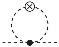
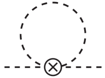
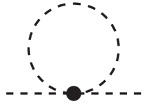
(a)		(b)		(c)

Figure 1: One loop diagrams contributing to the mesonic matrix elements of twist-two operators. The filled circle denotes a vertex from the chiral Lagrangian while the crossed circle corresponds to the twist-two operator. Diagram (c) denotes the wave function renormalisation.

Therefore at NLO, the vector GPD form factors will have the form:

$$A^{(A)}_{m+1,j}(t)=A^{(A)}_{m+1,j}+A^{(A,a)}_{m+1,j}M^{2}+A^{(A,b)}_{m+1,j}t+\text{loop\, contributions},$$ (30)

where $A^{(A)}_{m+1,j}$ is the bare matrix element determined in terms of the leading order LECs $a_{m+1,j}^{A}$, and $A^{(A,a)}_{m+1,j}$ and $A^{(A,b)}_{m+1,j}$ can be expressed in terms of linear combinations of the LECs accompanying the various NLO operators and absorb divergences from the loop contributions (in general this renders these terms renormalisation scale dependent). A similar expression holds for the tensor GPD form factors.

In the following subsections, we present results for the various matrix elements in the SU(4$|$2) isospin limit case, $m_{d}=m_{u}$ and $m_{l}=m_{j}$. In this limit, only the valence-valence meson mass, $M_{uu}=M_{\pi}$, and the valence-sea meson mass, $M_{uj}^{2}=M_{\pi}^{2}-\frac{1}{2}\delta_{uj}^{2}$, enter. Here $\delta_{uj}^{2}/2\lambda$ is the mass splitting between $u$ and $j$ quarks and results in SU(2) are easily obtained by setting $\delta_{uj}\to 0$ (these results are given in Appendix B).

IV.1 Isoscalar-vector operators

In the partially-quenched theory, the pion matrix elements of the isoscalar-vector operators have the form

$$\langle\pi^{+}|{\cal O}^{(m)}_{0}|\pi^{+}\rangle = 2\left(1-(-1)^{m}\right)\sum_{j=0,\rm even}^{m}a^{(0)}_{m+1,j}\left[(2\overline{P}\cdot u)^{m-j+1}(\Delta\cdot u)^{j}-(\Delta\cdot u)^{m+1}\right]$$

$$-\frac{\left(1-(-1)^{m}\right)}{48f^{2}\pi^{2}}(u\cdot\Delta)^{m+1}\sum_{j=0,\rm even}^{m}a^{(0)}_{m+1,j}\int_{-1}^{1}d\alpha\Bigg{\{}\frac{12\left(1-\alpha^{m+1-j}\right)\delta_{{uj}}^{2}M_{\pi}^{2}}{4M_{\pi}^{2}+t\left(\alpha^{2}-1\right)}$$

$$\hskip 14.22636pt+3\left(1-\alpha^{m+1-j}\right)\log\left[\frac{M_{\pi}^{2}+\frac{1}{4}t\left(\alpha^{2}-1\right)}{\mu^{2}}\right]M_{\pi}^{2}+\log\left[\frac{M_{uj}^{2}+\frac{1}{4}t\left(\alpha^{2}-1\right)}{\mu^{2}}\right]$$

$$\hskip 14.22636pt\times\left(t\left((j-m-4)\alpha^{2}-j+m+8\right)\alpha^{m+1-j}+4\left((j-m-2)\alpha^{m+1-j}+1\right)M_{{uj}}^{2}+t\left(3\alpha^{2}-7\right)\right)\Bigg{\}}\,,$$

for $m$ odd and vanish for $m$ even. Note that above and in what follows, we have suppressed analytic dependence of matrix elements on $M_{\pi}^{2}$, $M_{uj}^{2}$ and $t$. The first term in the braces arises from a double-pole propagator in Figure 1(a) and gives enhanced quark mass dependence. The QCD limit is easily obtained by setting $\delta_{uj}=0$ and $M_{uj}\to M_{\pi}$.

Decomposing this result leads to the following structure for the GPD form factors ($m$ odd):

$$A^{(0)}_{m+1,j}(t) = A^{(0)}_{m+1,j}+A^{(0,a)}_{m+1,j}M_{\pi}^{2}+\tilde{A}^{(0,a)}_{m+1,j}M_{uj}^{2}+A^{(0,b)}_{m+1,j}t,\ \text{for}\ j\leq m\,,$$ (32)

with no non-analytic dependence, and ($m$ odd)

$$C^{(0)}_{m+1}(t) = C^{(0)}_{m+1}+\frac{C^{(0)}_{m+1}}{96\pi^{2}f^{2}}\int_{-1}^{1}d\alpha\ \Bigg{\{}\frac{12\delta_{uj}^{2}M_{\pi}^{2}}{4M_{\pi}^{2}+t(\alpha^{2}-1)}+3M_{\pi}^{2}\log\left[\frac{M_{\pi}^{2}-\frac{t}{4}(1-\alpha^{2})}{\mu^{2}}\right]$$

$$\hskip 28.45274pt+((3\alpha^{2}-7)t+4M_{uj}^{2})\log\left[\frac{M_{uj}^{2}-\frac{t}{4}(1-\alpha^{2})}{\mu^{2}}\right]\Bigg{\}}+C^{(0,a)}_{m+1}M_{\pi}^{2}+\tilde{C}^{(0,a)}_{m+1}M_{uj}^{2}+C^{(0,b)}_{m+1}t$$

$$+\frac{1}{192\pi^{2}f^{2}}\sum_{j=0,\text{even}}^{m}2^{j-m}A^{(0)}_{m+1,j}\int_{-1}^{1}d\alpha\ \alpha^{m-j+1}\Bigg{\{}\frac{12\delta_{uj}^{2}M_{\pi}^{2}}{4M_{\pi}^{2}+t(\alpha^{2}-1)}+3M_{\pi}^{2}\log\left[\frac{M_{\pi}^{2}-\frac{t}{4}(1-\alpha^{2})}{\mu^{2}}\right]$$

$$\hskip 28.45274pt+\left(t(3\alpha^{2}-7)+4M_{uj}^{2}+4(m-j+1)\left(M_{uj}^{2}-\frac{t}{4}(1-\alpha^{2})\right)\right)\log\left[\frac{M_{uj}^{2}-\frac{t}{4}(1-\alpha^{2})}{\mu^{2}}\right]\Bigg{\}}\,,$$

where the LECs and the bare form-factors are related by $C_{m+1}^{(0)}=-\sum_{j=0,\text{even}}^{m}a_{m+1,j}^{(0)}$ and $A_{m+1,j}^{(0)}=2^{m-j+1}a_{m+1,j}^{(0)}$. The $\pi^{-}$ and $\pi^{0}$ results are identical and, with appropriate changes in normalisation, the QCD limits of these results agree with those in Refs. Kivel and Polyakov (2002); Diehl et al. (2005) using integration by parts and noting that $\sum_{j,{\rm even}}2^{j}A^{(0)}_{m+1,j}=0$ (the results for the gravitational form-factors, $A_{2,0}(t)$ and $C_{2}(t)$, also agree with previous calculations Donoghue and Leutwyler (1991)). In the partially quenched case, this form-factor leads to an enhanced divergence in the pion gravitational radius $\sim\delta_{uj}^{2}/M_{\pi}^{2}$ as opposed to $\ln M_{\pi}$ in QCD.

IV.2 Isovector-vector operators

The pion matrix elements of the isovector-vector operators have the form

$$\langle\pi^{+}|{\cal O}^{(m)}_{3}|\pi^{+}\rangle = (1+(-1)^{m})\sum_{j=0,\text{even}}^{m}a_{m+1,j}^{(3)}\Bigg{\{}2(2\overline{P}\cdot u)^{m-j+1}(\Delta\cdot u)^{j}\left(1-\frac{1}{8\pi^{2}f^{2}}M_{uj}^{2}\ \log\left[\frac{M_{uj}^{2}}{\mu^{2}}\right]\right)$$ (34)

$$-\frac{1}{8\pi^{2}f^{2}}\ (2\overline{P}\cdot u)(\Delta\cdot u)^{m}\left(\frac{t}{2}\int_{-1}^{1}d\alpha\ \alpha^{m-j+2}\ \text{log}\left[\frac{M_{uj}^{2}-\frac{t}{4}(1-\alpha^{2})}{\mu^{2}}\right]-2M_{uj}^{2}\text{log}\left[\frac{M_{uj}^{2}}{\mu^{2}}\right]\right)\Bigg{\}}\,,$$

for even $m$. This leads to the following structure for the GPD form factors:

$$A^{(3)}_{m+1,j}(t) = A^{(3)}_{m+1,j}\left(1-\frac{M_{uj}^{2}}{8\pi^{2}f^{2}}\text{log}\left(\frac{M_{uj}^{2}}{\mu^{2}}\right)\right)+A^{(3,a)}_{m+1,j}M_{\pi}^{2}+\tilde{A}^{(3,a)}_{m+1,j}M_{uj}^{2}+A^{(3,b)}_{m+1,j}t,\ \text{for}\ j\leq m-2\,,$$ (35)

and

$$A^{(3)}_{m+1,m}(t) = A^{(3)}_{m+1,m}\left(1-\frac{M_{uj}^{2}}{8\pi^{2}f^{2}}\text{log}\left(\frac{M_{uj}^{2}}{\mu^{2}}\right)\right)+A^{(3,a)}_{m+1,m}M_{\pi}^{2}+\tilde{A}^{(3,a)}_{m+1,m}M_{uj}^{2}+A^{(3,b)}_{m+1,m}t$$

$$+\sum_{j=0,\text{even}}^{m}\frac{2^{j-m}A_{m+1,j}^{(3)}}{8\pi^{2}f^{2}}\left\{M_{uj}^{2}\text{log}\left[\frac{M_{uj}^{2}}{\mu^{2}}\right]-\frac{t}{4}\int_{-1}^{1}d\alpha\ \alpha^{m-j+2}\ \text{log}\left[\frac{M_{uj}^{2}-\frac{t}{4}(1-\alpha^{2})}{\mu^{2}}\right]\right\}\,,$$

using $a_{m+1,j}^{(3)}=2^{j-m-1}A_{m+1,j}^{(3)}$. The $\pi^{-}$ results are related to these by factors of $-1$ and those in the $\pi^{0}$ vanish. The LECs $A_{1,0}^{(3,a)}$ and $\tilde{A}_{1,0}^{(3,a)}$ vanish by current conservation and $A_{1,0}^{(3)}=1$. These results can be shown to agree with Ref. Diehl et al. (2005); Kivel and Polyakov (2002) (and earlier results in the case of the vector-isovector form-factor, $A_{1,0}^{(3)}(t)$) using integration by parts and noting the different normalisations.

In the partially-quenched theory, isospin is not a good quantum number (the SU(4$|$2) adjoint matrices are given in Eq. (5)) and the odd-$m$ matrix elements are also non-zero. These take the form ($\pi^{-}$ and $\pi^{0}$ are identical to the $\pi^{+}$)

$$\langle\pi^{+}|{\cal O}^{(m)}_{3}|\pi^{+}\rangle_{m\rm\,odd} = \frac{\left(1-(-1)^{m}\right)}{8f^{2}\pi^{2}}({q_{j}}+{q_{k}})\sum_{j=0,\rm even}^{m}a^{(3)}_{m+1,j}$$

$$\hskip 14.22636pt\times\Bigg{\{}\frac{(u\cdot\Delta)^{m+1}}{24}\int_{-1}^{1}\frac{d\alpha}{\alpha^{j}}\Bigg{[}\frac{8\left(2\alpha^{j}+3\left(\alpha^{2}-1\right)\alpha^{m+1}\right)M_{\pi}^{2}\delta_{{uj}}^{4}}{\left(4M_{\pi}^{2}+t\left(\alpha^{2}-1\right)\right)^{2}}-\frac{24\left(\alpha^{j}-\alpha^{m+1}\right)M_{\pi}^{2}\delta_{{uj}}^{2}}{4M_{\pi}^{2}+t\left(\alpha^{2}-1\right)}$$

$$\hskip 42.67912pt+\log\left(\frac{M_{\pi}^{2}+\frac{1}{4}t\left(\alpha^{2}-1\right)}{\mu^{2}}\right)G(M_{\pi})-\log\left(\frac{M_{{uj}}^{2}+\frac{1}{4}t\left(\alpha^{2}-1\right)}{\mu^{2}}\right)G(M_{uj})\Bigg{]}$$

$$\hskip 28.45274pt+\left[(u\cdot\Delta)^{m+1}-(2\overline{P}\cdot u)^{m+1-j}(u\cdot\Delta)^{j}\right]\left(\log\left(\frac{M_{\pi}^{2}}{\mu^{2}}\right)M_{\pi}^{2}-\log\left(\frac{M_{{uj}}^{2}}{\mu^{2}}\right)M_{{uj}}^{2}\right)\Bigg{\}}\,,$$

where $G(M)=\left(t\left(3\alpha^{2}-7\right)\alpha^{j}+t\left((j-m-4)\alpha^{2}-j+m+8\right)\alpha^{m+1}+4\left(\alpha^{j}+(j-m-2)\alpha^{m+1}\right)M^{2}\right)$. Note that this matrix element vanishes in the QCD limit and the sea-isospin limit where $q_{j}=-q_{k}$, in which foreseeable lattice calculations would be performed. Consequently, we do not present the form-factors that result.

IV.3 Tensor operators

For $m$ odd, the matrix elements of the tensor operator are given by:

$$\langle\pi^{+}|{\cal O}^{(m)}_{T}|\pi^{+}\rangle = 8(1-(-1)^{m})\overline{P}\cdot ur\cdot\Delta\sum_{j=0,\rm even}^{m}b_{m+1,j}(2\overline{P}\cdot u)^{m-j}(u\cdot\Delta)^{j}\Bigg{\{}(1+y)\left[1+\frac{M_{uj}^{2}}{12\pi^{2}f^{2}}\log\left(\frac{M_{uj}^{2}}{\mu^{2}}\right)\right]$$

$$\hskip 42.67912pt-\frac{1}{48f^{2}\pi^{2}}\Bigg{[}2(3({q_{3}}+{q_{4}})+5(1+y))\log\left(\frac{M_{{uj}}^{2}}{\mu^{2}}\right)M_{{uj}}^{2}$$

$$\hskip 85.35826pt-3\log\left(\frac{M_{\pi}^{2}}{\mu^{2}}\right)\left((2({q_{3}}+{q_{4}})-(1+y))M_{\pi}^{2}+(1+y)\delta_{{uj}}^{2}\right)\Bigg{]}\Bigg{\}}\,,$$

which simplifies considerably in the QCD limit. These matrix elements vanish if the charge matrix is isovector in both the sea and valence sectors. Matrix elements in the $\pi^{-}$ and $\pi^{0}$ are identical.

For $m$ even, the matrix elements are given by

$$\langle\pi^{+}|{\cal O}^{(m)}_{T}|\pi^{+}\rangle = 2(1-y)\overline{P}\cdot ur\cdot\Delta\sum_{j=0,\rm even}^{m}b_{m+1,j}\Bigg{\{}-4(u\cdot\Delta)^{j}\left((p\cdot u)^{m-j}-2(2\overline{P}\cdot u)^{m-j}+((p+\Delta)\cdot u)^{m-j}\right)$$ (39)

$$\hskip 28.45274pt\times\Bigg{[}1+\frac{M_{uj}^{2}}{12\pi^{2}f^{2}}\log\left(\frac{M_{uj}^{2}}{\mu^{2}}\right)+\frac{1}{48f^{2}\pi^{2}}\left[3\log\left(\frac{M_{\pi}^{2}}{\mu^{2}}\right)(M_{\pi}^{2}+\delta_{{uj}}^{2})-10\log\left(\frac{M_{uj}^{2}}{\mu^{2}}\right)M_{uj}^{2}\right]\Bigg{]}$$

$$-\frac{(u\cdot\Delta)^{m}}{16f^{2}\pi^{2}}\int_{-1}^{1}d\alpha\left(4M_{{uj}}^{2}+t\left(\alpha^{2}-1\right)\right)$$

$$\hskip 28.45274pt\times\left[\left(\frac{1-\alpha}{2}\right)^{m-j}-2\alpha^{m-j}+\left(\frac{1+\alpha}{2}\right)^{m-j}\right]\log\left(\frac{M_{{uj}}^{2}+\frac{1}{4}t\left(\alpha^{2}-1\right)}{\mu^{2}}\right)\Bigg{\}}\,,$$

vanishing in the isoscalar case. The $\pi^{-}$ matrix elements differ by an overall sign and the $\pi^{0}$ matrix elements vanish.

The results in Eqs. (IV.3) and (39) are easily converted into the various GPD form factors. For $m$ odd,

$$B^{T}_{m+1,j}(t) = B^{T,(0)}_{m+1,j}\Bigg{\{}\frac{(1+y)}{2}\left[1-\frac{M_{uj}^{2}}{8\pi^{2}f^{2}}\log\left(\frac{M_{{uj}}^{2}}{\mu^{2}}\right)-\frac{M_{\pi}^{2}-\delta_{uj}^{2}}{16\pi^{2}f^{2}}\log\left(\frac{M_{\pi}^{2}}{\mu^{2}}\right)\right]-\frac{q_{3}+q_{4}}{16\pi^{2}f^{2}}M_{uj}^{2}\log\left(\frac{M_{{uj}}^{2}}{\mu^{2}}\right)$$ (40)

$$\hskip 42.67912pt+\frac{q_{3}+q_{4}}{16\pi^{2}f^{2}}M_{\pi}^{2}\log\left(\frac{M_{{\pi}}^{2}}{\mu^{2}}\right)\Bigg{\}}+B^{T,(a)}_{m+1,j}M_{\pi}^{2}+\tilde{B}^{T,(a)}_{m+1,j}M_{uj}^{2}+B^{T,(b)}_{m+1,j}t\,,$$

for all $j$. Here $B^{T,(0)}_{m+1,j}=8\,2^{m-j}\Lambda_{\chi}b_{m+1,j}$ ($m$ odd).

While for $m$ even,

$$B^{T}_{m+1,j}(t) = B^{T,(0)}_{m+1,j}\frac{1-y}{2}\Bigg{\{}1+\frac{1}{16\pi^{2}f^{2}}\Bigg{[}\left(M_{\pi}^{2}+\delta_{uj}^{2}\right)\log\left(\frac{M_{\pi}^{2}}{\mu^{2}}\right)-2M_{uj}^{2}\log\left(\frac{M_{uj}^{2}}{\mu^{2}}\right)\Bigg{]}\Bigg{\}}$$ (41)

$$\hskip 28.45274pt+B^{T,(a)}_{m+1,j}M_{\pi}^{2}+\tilde{B}^{T,(a)}_{m+1,j}M_{uj}^{2}+B^{T,(b)}_{m+1,j}t\,,$$

for $j<m$, and

$$B^{T}_{m+1,m}(t) = B^{T,(0)}_{m+1,m}\frac{1-y}{2}\Bigg{\{}1+\frac{1}{16\pi^{2}f^{2}}\Bigg{[}\left(M_{\pi}^{2}+\delta_{uj}^{2}\right)\log\left(\frac{M_{\pi}^{2}}{\mu^{2}}\right)-2M_{uj}^{2}\log\left(\frac{M_{uj}^{2}}{\mu^{2}}\right)\Bigg{]}\Bigg{\}}$$ (42)

$$+\frac{1-y}{32f^{2}\pi^{2}}\sum_{j=0,\rm even}^{m}B^{T,(0)}_{m+1,j}\int_{-1}^{1}d\alpha\left(M_{{uj}}^{2}+\frac{t}{4}\left(\alpha^{2}-1\right)\right)\left[\frac{\alpha}{2}\right]^{m-j}\log\left(\frac{M_{{uj}}^{2}+\frac{1}{4}t\left(\alpha^{2}-1\right)}{\mu^{2}}\right)$$

$$+B^{T,(a)}_{m+1,m}M_{\pi}^{2}+\tilde{B}^{T,(a)}_{m+1,m}M_{uj}^{2}+B^{T,(b)}_{m+1,m}t\,,$$

where $B_{m+1,j}^{T,(0)}=-8\Lambda_{\chi}\left[\sum_{k=0,\rm even}^{m}\left({\tiny\begin{array}[]{c}m-k\\ j-k\end{array}}\right)2^{k-j}b_{m+1,k}-2^{m-j}b_{m+1,j}\right]$ ($m$ even) is the leading order result for the form-factor. In the QCD limit, these result reproduce those of Ref. Diehl et al. (2006a) [Eqs. (106) and (128) therein]. As these results are insensitive to the sea-quark charges, these form-factors can be calculated in lattice QCD without disconnected quark loops.

V Finite Volume Effects

The space-time lattices used in numerical simulations are of finite extent by necessity, and consequently, lattice results differ from those of the physical (infinite volume) world even at the physical quark masses. For sufficiently large volumes, these effects can be incorporated into the effective field theory approach, allowing infinite volume results to be extracted from the finite volume (FV) lattice simulations. Here we shall consider a hyper-rectangular box of dimensions $L^{3}\times T$ with $T\gg L$ as appropriate for most current lattice calculations. Imposing periodic boundary conditions on mesonic fields leads to quantised momenta $k=(k_{0},{\vec{k}})$, ${\vec{k}}=\frac{2\pi}{L}{\vec{j}}=\frac{2\pi}{L}(j_{1},j_{2},j_{3})$ with $j_{i}\in\mathbb{Z}$, but $k_{0}$ treated as continuous. On such a finite volume, spatial momentum integrals are replaced by sums over the available momentum modes. This leads to modifications of the infinite volume results presented in the previous section; the various functions arising from loop integrals are replaced by their FV counterparts. In a system where $M_{\pi}L\gg 1$, finite volume effects are predominantly from Goldstone mesons propagating to large distances where they are sensitive to boundary conditions and can even “wrap around the world”. Since the lowest momentum mode of the Goldstone propagator is $\sim\exp(-M_{\pi}L)$ in position space, finite volume effects will behave as a polynomial in $1/L$ times this exponential provided no multi-particle thresholds are reached, that is for $t<4M_{\pi}^{2}$. For $t\geq 4M_{\pi}^{2}$, volume effects that are polynomial in inverse powers of $L$ are expected, however for realistic lattice calculations, such momentum transfers are too large to be described in  and we neglect the resulting complications in our analysis.

The finite volume effects in the diagrams of Fig. 1(b) and (c) arising from the operators that contribute at infinite volume are well known. However the effects in Fig. 1(a) are made more complicated by the non-trivial numerator structure of the integral/sum and the requisite details for their evaluation are given in Appendix A. The final forms for the finite volume versions of our results are given below. In most cases, these replacements of spatial momentum integrals by sums would complete the calculation of finite volume effects. However for the GPD form-factors, there are additional complications that arise from operators whose contributions vanish in infinite volume but which give non-zero contributions at finite volume. To see this, we concentrate on the vector case and reconsider the operator in Eq. (26) (note there is some redundancy of terms in this operator). Naïvely, this operator would contribute through diagram (b) in Fig. 1. As discussed in Section III, there is no contribution at infinite volume as the each of the pion fields coming from this operator must have a non-zero number of derivatives acting on it. Combining $u^{2}=0$ (or equivalently, the definite Lorentz transformation properties of the twist-two, spin-$n$, operators) and the symmetric range of integration, terms with derivatives inside the loop in Fig. 1(b) give no contribution.

In the finite volumes discussed here, Lorentz symmetry (or O(4) symmetry in Euclidean space as relevant in lattice calculations) is explicitly broken by the imposition of the boundary conditions (in a $L^{3}\times T$ periodic box, arbitrary Lorentz boosts do not leave the system invariant). As a result, the arguments used to discard the operators in Eq. (26) break down ($\frac{1}{L^{3}}\int dq_{0}\sum_{\vec{q}}\frac{(u.q)^{2}}{(q^{2}-m^{2})^{j}}\neq 0$ at finite volume) and their contributions, which must vanish as $L\to\infty$, need to be incorporated to correctly describe finite volume lattice calculations Consequently, one must include the functional dependence arising from operators such as those in Eq. (26) in any fit to lattice data and determine the relevant combinations of the $a^{A,2}_{m,j_{1},j_{2},j_{3}}$ as well as the $a_{m+1,j}^{A}$ before discarding the former (we have no interest in these LECs for the matrix elements we want to extract, however they would contribute in more complicated matrix elements such as two pion matrix elements of twist-two operators) in extracting the infinite volume result. In general this is a very intricate task as the functional dependence produced by these operators in the contribution of Fig. 1(b) to the matrix element of ${\cal O}^{(m)}_{A}$ is

$$\sum_{l=2,\,{\rm even}}^{n}\gamma_{n,l}u_{\mu_{1}}\ldots u_{\mu_{l}}\int dk_{0}\frac{1}{L^{3}}\sum_{\vec{k}}\frac{k^{\mu_{1}}\ldots k^{\mu_{l}}-{\rm tr}}{k^{2}-m^{2}}$$ (43)

where the parameters $\gamma_{n,l}$ are linear combinations of those that enter in Eq. (26). However for the low moments ($m<4$) that are accessible in current lattice calculations, these subtractions can be performed.

A number of additional aspects of Lorentz symmetry violation at finite volume are worth noting. Firstly, these effects did not contribute in the nucleon twist-two matrix elements at finite volume at NLO Detmold and Lin (2005), but will contribute at higher orders in the chiral expansion in a similar way as they enter here. We also note that moments of distribution amplitudes (given by meson to vacuum matrix elements of related quark-bilinear operators) will suffer from similar complications at finite volume and the absence of non-analytic quark mass dependence at NLO found in Ref. Chen and Stewart (2004) at infinite volume will not persist. Secondly, as shown in Ref. Gasser and Leutwyler (1988), no new operators can appear at finite volume otherwise their LECs would necessarily depend on $L^{-1}$, an infrared scale. In the case described above, the operator is present both at finite volume and infinite volume, but doesn’t contribute to the matrix elements we consider in the latter case. A final related effect of the finite volume is that Lorentz symmetry can no longer be used to decompose the matrix elements of the twist-two operators. At finite volume, additional structures that violate Lorentz symmetry can appear in the decomposition of the matrix elements in Eqs. (10)–(13). The form factors of such terms vanish as $L\to\infty$ and we ignore them here but care must be taken to correctly extract the form-factors in Eqs. (10–13) without pollution from these additional Lorentz non-invariant form-factors.

V.1 Finite volume matrix elements

With the preceding remarks in mind, the finite volume versions of the results of the previous section are given by the following matrix elements:

$$\langle\pi^{+}|{\cal O}^{(m)}_{0}|\pi^{+}\rangle^{m\,\rm odd}_{\rm FV} = 2(1-(-1)^{m})\sum_{j=0,{\rm even}}^{m}a^{(0)}_{m+1,j}\Bigg{\{}\left((2\overline{P}\cdot u)^{m+1-j}(u\cdot\Delta)^{j}-(u\cdot\Delta)^{m+1}\right)$$

$$+\frac{(u\cdot\Delta)^{m+1}}{3f^{2}}\Bigg{[}-2\left(2M_{\pi}^{2}-\delta_{uj}^{2}+2t\right)K_{0,0,0,0,0}^{{uj}}$$

$$\hskip 14.22636pt+3M_{\pi}^{2}\left(K_{0,0,0,0,0}^{{uu}}+\delta_{{uj}}^{2}\left(K_{0,0,0,0,0}^{{uu1}}+K_{0,0,0,0,0}^{{uu2}}\right)\right)+4\left(K_{0,0,0,1,0}^{{uj}}+K_{0,1,0,0,0}^{{uj}}\right)$$

$$\hskip 14.22636pt-\sum_{k=0}^{m+1-j}\left({\tiny\begin{array}[]{c}m+1-j\\ k\end{array}}\right)2^{k}(u\cdot\Delta)^{-k}\Big{(}-2\left(2M_{\pi}^{2}-\delta_{uj}^{2}+2t\right)K_{k,0,0,0,0}^{{uj}}$$

$$\hskip 14.22636pt+3M_{\pi}^{2}\left(K_{k,0,0,0,0}^{{uu}}+\delta_{{uj}}^{2}\left(K_{k,0,0,0,0}^{{uu1}}+K_{k,0,0,0,0}^{{uu2}}\right)\right)+4\left(K_{k,0,0,1,0}^{{uj}}+K_{k,1,0,0,0}^{{uj}}\right)\Big{)}\Bigg{]}\Bigg{\}}\,,$$

$$\langle\pi^{+}|{\cal O}^{(m)}_{3}|\pi^{+}\rangle^{m\,\rm even}_{\rm FV} = 2(1+(-1)^{m})\sum_{j=0,{\rm even}}^{m}a^{(3)}_{m+1,j}\Bigg{\{}(2\overline{P}\cdot u)^{m+1-j}(u\cdot\Delta)^{j}\left(1-\frac{2}{f^{2}}J_{u,j}\right)$$ (51)

$$\hskip 113.81102pt-\frac{2}{f^{2}}\sum_{k=0}^{m+1-j}\left({\tiny\begin{array}[]{c}m+1-j\\ k\end{array}}\right)2^{k}(u\cdot\Delta)^{m+1-k}\left(K_{k,0,0,1,0}^{{uj}}+2K_{k,0,1,0,0}^{{uj}}\right)\Bigg{\}}\,,$$

$$\langle\pi^{+}|{\cal O}^{(m)}_{3}|\pi^{+}\rangle^{m\,\rm odd}_{\rm FV} = \frac{\left(1-(-1)^{m}\right)}{3f^{2}}\left(q_{j}+q_{k}\right)\sum_{j=0,{\rm even}}^{m}a^{(3)}_{m+1,j}\Bigg{\{}(u\cdot\Delta)^{m+1}\Big{[}-\left(2M_{\pi}^{2}-\delta_{{uj}}^{2}+2t\right)K_{0,0,0,0,0}^{{uj}}$$

$$\hskip 28.45274pt+2\left(M_{\pi}^{2}+t\right)K_{0,0,0,0,0}^{{uu}}+3M_{\pi}^{2}\delta_{{uj}}^{2}\left(K_{0,0,0,0,0}^{{uu1}}+K_{0,0,0,0,0}^{{uu2}}+\delta_{{uj}}^{2}K_{0,0,0,0,0}^{{uu3}}\right)$$

$$\hskip 28.45274pt+2\left(K_{0,0,0,1,0}^{{uj}}-K_{0,0,0,1,0}^{{uu}}+K_{0,1,0,0,0}^{{uj}}-K_{0,1,0,0,0}^{{uu}}\right)\Big{]}$$

$$-\sum_{k=0}^{m+1-j}\left({\tiny\begin{array}[]{c}m+1-j\\ k\end{array}}\right)2^{k}(u\cdot\Delta)^{m+1-k}\Big{[}-\left(2M_{\pi}^{2}-\delta_{{uj}}^{2}+2t\right)K_{k,0,0,0,0}^{{uj}}+2\left(M_{\pi}^{2}+t\right)K_{k,0,0,0,0}^{{uu}}$$

$$\hskip 28.45274pt+3M_{\pi}^{2}\delta_{{uj}}^{2}\left(K_{k,0,0,0,0}^{{uu1}}+K_{k,0,0,0,0}^{{uu2}}+\delta_{{uj}}^{2}K_{k,0,0,0,0}^{{uu3}}\right)$$

$$\hskip 28.45274pt+2\left(K_{k,0,0,1,0}^{{uj}}-K_{k,0,0,1,0}^{{uu}}+K_{k,1,0,0,0}^{{uj}}-K_{k,1,0,0,0}^{{uu}}\right)\Big{]}$$

$$+6\left(2^{-j+m+1}(\overline{P}\cdot u)^{m+1-j}(u\cdot\Delta)^{j}-(u\cdot\Delta)^{m+1}\right)\left(J_{u,j}-J_{u,u}\right)\Bigg{\}}\,,$$

$$\langle\pi^{+}|{\cal O}^{(m)}_{T}|\pi^{+}\rangle^{m\,\rm even}_{\rm FV} = 2(1-y)\overline{P}\cdot ur\cdot\Delta\sum_{j=0,{\rm even}}^{m}\frac{B^{T\,(0)}_{m+1,j}}{\Lambda_{\chi}}(u\cdot\Delta)^{j}(\overline{P}\cdot u)^{m-j}\left(1+\frac{1}{f^{2}}(L_{u,u}\delta_{{uj}}^{2}-2J_{u,j}+J_{u,u})\right)$$ (59)

$$-\frac{16(1-y)}{f^{2}}\sum_{j=0,{\rm even}}^{m}b_{m+1,j}\Bigg{\{}-r\cdot\Delta(u\cdot\Delta)^{j}\left(K_{m+1-j,0,0,1,0}^{{uj}}+2K_{m+1-j,0,1,0,0}^{{uj}}\right)$$

$$\hskip 56.9055pt+(u\cdot\Delta)^{j+1}\left(K_{m-j,0,0,1,1}^{{uj}}+2K_{m-j,0,1,0,1}^{{uj}}\right)$$

$$\hskip 28.45274pt+\sum_{k=0}^{m-j}\left({\tiny\begin{array}[]{c}m-j\\ k\end{array}}\right)\left(2^{k+1}-1\right)(u\cdot\Delta)^{m-k}\Bigg{[}r\cdot\Delta\left(K_{k+1,0,0,1,0}^{{uj}}+2K_{k+1,0,1,0,0}^{{uj}}\right)$$

$$\hskip 56.9055pt-u\cdot\Delta\left(K_{k,0,0,1,1}^{{uj}}+2K_{k,0,1,0,1}^{{uj}}\right)\Bigg{]}\Bigg{\}}\,,$$

and

$$\langle\pi^{+}|{\cal O}^{(m)}_{T}|\pi^{+}\rangle^{m\,\rm odd}_{\rm FV} = 8r\cdot\Delta\sum_{j=0,{\rm even}}^{m}(2\overline{P}\cdot u)^{m+1-j}(u\cdot\Delta)^{j}b_{m+1,j}\Bigg{[}(y+1)\left(1-\frac{1}{f^{2}}(2J_{u,j}+J_{u,u}-\delta_{{uj}}^{2}L_{u,u})\right)$$

$$\hskip 56.9055pt-\frac{2}{f^{2}}\left(q_{3}+q_{4}\right)\left(J_{u,j}-J_{u,u}\right)\Bigg{]}$$

$$-\frac{16(u\cdot\Delta)^{m}}{3f^{2}}\sum_{j=0,{\rm even}}^{m}b_{m+1,j}\sum_{k=0}^{m-j}\left({\tiny\begin{array}[]{c}m-j\\ k\end{array}}\right)2^{k}(u\cdot\Delta)^{-k}$$

$$\hskip 5.69054pt\times\Bigg{\{}u\cdot\Delta\Bigg{[}\left(2M_{\pi}^{2}-\delta_{uj}^{2}+2t\right){\cal Q}_{34}K_{k,0,0,0,1}^{{uj}}-2{\cal Q}_{34}K_{k,0,0,1,1}^{{uj}}-2{\cal Q}_{34}K_{k,1,0,0,1}^{{uj}}$$

$$\hskip 28.45274pt+M_{\pi}^{2}\Big{(}{\cal Q}_{34}K_{k,0,0,0,1}^{{uj}}-{\cal Q}_{34}^{\prime\prime}K_{k,0,0,0,1}^{{uu}}-3\left(q_{3}+q_{4}\right)\delta_{{uj}}^{2}\left(K_{k,0,0,0,1}^{{uu1}}+K_{k,0,0,0,1}^{{uu2}}\right)$$

$$\hskip 28.45274pt+3{\cal Q}_{34}^{\prime}\delta_{{uj}}^{4}K_{k,0,0,0,1}^{{uu3}}\Big{)}-2{\cal Q}_{34}^{\prime}\left(-tK_{k,0,0,0,1}^{{uu}}+K_{k,0,0,1,1}^{{uu}}+K_{k,1,0,0,1}^{{uu}}\right)\Bigg{]}$$

$$\hskip 14.22636pt-r\cdot\Delta\Bigg{[}\left(2M_{\pi}^{2}-\delta_{uj}^{2}+2t\right){\cal Q}_{34}K_{k+1,0,0,0,0}^{{uj}}-2{\cal Q}_{34}K_{k+1,0,0,1,0}^{{uj}}-2{\cal Q}_{34}K_{k+1,1,0,0,0}^{{uj}}$$

$$\hskip 28.45274pt+M_{\pi}^{2}\Big{(}{\cal Q}_{34}K_{k+1,0,0,0,0}^{{uj}}-{\cal Q}_{34}^{\prime\prime}K_{k+1,0,0,0,0}^{{uu}}-3\left(q_{3}+q_{4}\right)\delta_{{uj}}^{2}\left(K_{k+1,0,0,0,0}^{{uu1}}+K_{k+1,0,0,0,0}^{{uu2}}\right)$$

$$\hskip 28.45274pt+3{\cal Q}_{34}^{\prime}\delta_{{uj}}^{4}K_{k+1,0,0,0,0}^{{uu3}}\Big{)}-2{\cal Q}_{34}^{\prime}\left(-tK_{k+1,0,0,0,0}^{{uu}}+K_{k+1,0,0,1,0}^{{uu}}+K_{k+1,1,0,0,0}^{{uu}}\right)\Bigg{]}\Bigg{\}}\,,$$

where ${\cal Q}_{34}=1+y+q_{3}+q_{4}$, ${\cal Q}_{34}^{\prime}=1+y-q_{3}-q_{4}$ and ${\cal Q}_{34}^{\prime\prime}=1+y+2q_{3}+2q_{4}$. Note that the entire last sum in the above expression vanishes identically at infinite volume.

Here

$$J_{a,b}=\int\frac{dq_{0}}{2\pi}\frac{1}{L^{3}}\sum_{\vec{q}}\frac{i}{q^{2}-M_{ab}^{2}+i\epsilon}, L_{a,b}=\int\frac{dq_{0}}{2\pi}\frac{1}{L^{3}}\sum_{\vec{q}}\frac{i}{(q^{2}-M_{ab}^{2}+i\epsilon)^{2}},$$ (64)

and

$$K_{i,a,b,c,d}^{fg}={\cal K}_{i,a,b,c,d}^{f,g;1,1},\quad K_{i,a,b,c,d}^{fg1}={\cal K}_{i,a,b,c,d}^{f,g;2,1},\quad K_{i,a,b,c,d}^{fg2}={\cal K}_{i,a,b,c,d}^{f,g;1,2},\quad K_{i,a,b,c,d}^{fg3}={\cal K}_{i,a,b,c,d}^{f,g;2,2},\quad$$ (65)

where

$${\cal K}_{i,a,b,c,d}^{f,g;n_{1},n_{2}} = -i\int\frac{dq_{0}}{2\pi}\frac{1}{L^{3}}\sum_{\vec{q}}\frac{(u\cdot q)^{i}(q^{2})^{a}(p\cdot q)^{b}(q\cdot\Delta)^{c}(q\cdot r)^{d}}{(q^{2}-M_{fg}^{2}+i\epsilon)^{n_{1}}((q+\Delta)^{2}-M_{fg}^{2}+i\epsilon)^{n_{2}}}$$ (66)

which in turn is simply represented in terms of the functions appearing in Appendix A.

Since the external momenta $p=\overline{P}-\Delta/2$, $\Delta$, $u$ and $r$ occur in the various integrals/sums, it is not possible to decompose these matrix elements into form-factors without specifying to a particular $m$.

VI Discussion

The results for the quark mass and volume dependence of the moments of the pion GPDs presented above are useful in extrapolating lattice data at small $t$ in the chiral regime (the range of volumes and pion masses for which the chiral expansion is convergent) to the physical world. Although subtleties not seen in simpler quantities arise at finite volume that complicate the extraction of the infinite volume results for the twist-two matrix elements, we have outlined a procedure by which the extrapolation can be performed reliably. The knowledge of the meson GPDs that can be obtained by combining our results with lattice calculations will be useful in comparison to, and as a complement to, experiment.

Appendix A Finite volume functions

The functions used in our results at finite volume can be built from the following basic structure

$${\cal J}_{\alpha,n_{1},n_{2}}^{i_{1}\ldots i_{\beta}}(m_{1},m_{2},\Delta;L) = -i\int\frac{d\,q_{0}}{2\pi}\frac{1}{L^{3}}\sum_{\vec{q}}\frac{q_{0}^{2\alpha}\vec{q}^{i_{1}}\ldots\vec{q}^{i_{\beta}}}{(q^{2}-m_{1}^{2}+i\epsilon)^{n_{1}}((q+\Delta)^{2}-m_{2}^{2}+i\epsilon)^{n_{2}}}$$ (67)

$$= -\frac{1}{L^{3}\,\Gamma(n_{1})\Gamma(n_{2})}\int_{0}^{1}d\,x\sum_{\vec{k}}\frac{\partial^{n_{1}+n_{2}-1}}{\partial k_{0}^{n_{1}+n_{2}-1}}\left[\frac{k_{0}^{2\alpha}\vec{k}^{i_{1}}\ldots\vec{k}^{i_{\beta}}}{\left[k_{0}+\hat{k}_{0}\right]^{n_{1}+n_{2}}}\right]_{k_{0}=\hat{k}_{0}}\,,$$

where

$$\hat{k}_{0}=\sqrt{|\vec{k}|^{2}+2(1-x)\vec{k}\cdot\vec{\Delta}+(1-x)|\vec{\Delta}|^{2}+xm_{1}^{2}+(1-x)m_{2}^{2}}\,,$$

after performing the energy integral by contour integration. As an example, we find that

$$K^{ab}_{j,0,0,0,1} = \sum_{k=0}^{\lfloor\frac{j}{2}\rfloor}(-1)^{j-k-1}\left[u_{0}^{2k+1}\vec{u}^{i_{1}}\ldots\vec{u}^{i_{j-k-1}}r_{0}{\cal J}_{k+1,1,1}^{i_{1},\ldots,i_{j-k-1}}-u_{0}^{2k}\vec{u}^{i_{1}}\ldots\vec{u}^{i_{j-k}}\vec{r}^{i_{j-k+1}}{\cal J}_{k,1,1}^{i_{1},\ldots,i_{j-k+1}}\right]\,.$$ (68)

It is possible to write down a general expression for the multiple derivative in Eq. (67) but since we only require $\{n_{1},n_{2}\}=\{1,1\},\{1,2\},\{2,1\},\{2,2\}$, it is easier to present each case explicitly. This leads to

$${\cal J}_{\alpha,1,1}^{i_{1}\ldots i_{\beta}}(m_{1},m_{2},\Delta;L) = -\frac{(2\alpha-1)}{4L^{3}\,}\int_{0}^{1}d\,x\,I_{\frac{3}{2}-\alpha}^{i_{1}\ldots i_{\beta}}\left[(1-x)\vec{\Delta},{\cal M}\right]\,,$$ (70)

$${\cal J}_{\alpha,1,2}^{i_{1}\ldots i_{\beta}}(m_{1},m_{2},\Delta;L) = -\frac{(4\alpha^{2}-8\alpha+3)}{8L^{3}\,}\int_{0}^{1}d\,x\,(1-x)I_{\frac{5}{2}-\alpha}^{i_{1}\ldots i_{\beta}}\left[(1-x)\vec{\Delta},{\cal M}\right]\,,$$ (71)

$${\cal J}_{\alpha,2,1}^{i_{1}\ldots i_{\beta}}(m_{1},m_{2},\Delta;L) = -\frac{(4\alpha^{2}-8\alpha+3)}{8L^{3}\,}\int_{0}^{1}d\,x\,x\,I_{\frac{5}{2}-\alpha}^{i_{1}\ldots i_{\beta}}\left[(1-x)\vec{\Delta},{\cal M}\right]\,,$$ (72)

$${\cal J}_{\alpha,2,2}^{i_{1}\ldots i_{\beta}}(m_{1},m_{2},\Delta;L) = -\frac{(8\alpha^{3}-36\alpha^{2}+46\alpha-15)}{16L^{3}\,}\int_{0}^{1}d\,x\,x(1-x)I_{\frac{7}{2}-\alpha}^{i_{1}\ldots i_{\beta}}\left[(1-x)\vec{\Delta},{\cal M}\right]\,,$$ (73)

where ${\cal M}=x(1-x)|\vec{\Delta}|^{2}+xm_{1}^{2}+(1-x)m_{2}^{2}$ and

$$I_{\beta}^{i_{1}\ldots i_{n}}(\vec{z},m) \equiv \sum_{\vec{q}}\frac{q^{i_{1}}\ldots q^{i_{n}}}{\left(|\vec{q}+\vec{z}|^{2}+m^{2}\right)^{\beta}}\,.$$ (74)

These sums can then be further simplified using the recurrence identity

$$I_{\beta}^{i_{1}\ldots i_{n}}(\vec{z},m) = -\frac{1}{2(\beta-1)}\frac{dI_{\beta-1}^{i_{1}\ldots i_{n-1}}}{dz_{i_{n}}}-z^{i_{n}}I_{\beta}^{i_{1}\ldots i_{n-1}}(\vec{z},m)$$ (75)

$$\longrightarrow (-1)^{n}\sum_{k=0}^{n}\sum_{\cal P}{\cal P}\left(\partial_{z}^{i_{1}}\ldots\partial_{z}^{i_{k}}z^{i_{k+1}}\ldots z^{i_{n}}\right)I_{\beta-k}(\vec{z},m)\,,$$

where ${\cal P}$ denotes a permutation of the orderings of the partial derivatives, $\partial_{z}^{i}=\frac{\partial}{\partial z^{i}}$, and the $z^{i}$’s, and the sum is over all such permutations. The remaining momentum sums have scalar summands and are simple to evaluate using the results of Ref. Sachrajda and Villadoro (2005) and the tracelessness condition. Divergences can be regulated using Epstein-Hurwitz zeta-function techniques Elizalde (1998).

Appendix B QCD form-factors

For easy reference, the non-vanishing, infinite volume form-factors in the SU(2) theory are given here.

In the vector-isoscalar case for $m$ odd,

$$A^{(0)}_{m+1,j}(t) = A^{(0)}_{m+1,j}+(A^{(0,a)}_{m+1,j}+\tilde{A}^{(0,a)}_{m+1,j})M_{\pi}^{2}+A^{(0,b)}_{m+1,j}t,\ \text{for}\ j\leq m\,,$$ (76)

and

$$C^{(0)}_{m+1}(t) = C^{(0)}_{m+1}+\frac{C^{(0)}_{m+1}}{96\pi^{2}f^{2}}\int_{-1}^{1}d\alpha((3\alpha^{2}-7)t+7M_{\pi}^{2})\log\left[\frac{M_{\pi}^{2}-\frac{t}{4}(1-\alpha^{2})}{\mu^{2}}\right]+(C^{(0,a)}_{m+1}+\tilde{C}^{(0,a)}_{m+1})M_{\pi}^{2}+C^{(0,b)}_{m+1}t$$

$$+\frac{1}{192\pi^{2}f^{2}}\sum_{j=0,\text{even}}^{m}2^{j-m}A^{(0)}_{m+1,j}$$

$$\hskip 17.07182pt\times\int_{-1}^{1}d\alpha\ \alpha^{m-j+1}\left(t(3\alpha^{2}-7)+7M_{\pi}^{2}+4(m-j+1)\left(M_{\pi}^{2}-\frac{t}{4}(1-\alpha^{2})\right)\right)\log\left[\frac{M_{\pi}^{2}-\frac{t}{4}(1-\alpha^{2})}{\mu^{2}}\right]\,.$$

In the vector-isovector case for $m$ even,

$$A^{(3)}_{m+1,j}(t) = A^{(3)}_{m+1,j}\left(1-\frac{M_{\pi}^{2}}{8\pi^{2}f^{2}}\text{log}\left(\frac{M_{\pi}^{2}}{\mu^{2}}\right)\right)+(A^{(3,a)}_{m+1,j}+\tilde{A}^{(3,a)}_{m+1,j})M_{\pi}^{2}+A^{(3,b)}_{m+1,j}t,\ \text{for}\ j\leq m-2\,,$$ (78)

and

$$A^{(3)}_{m+1,m}(t) = A^{(3)}_{m+1,m}\left(1-\frac{M_{\pi}^{2}}{8\pi^{2}f^{2}}\text{log}\left(\frac{M_{\pi}^{2}}{\mu^{2}}\right)\right)+(A^{(3,a)}_{m+1,m}+\tilde{A}^{(3,a)}_{m+1,m})M_{\pi}^{2}+A^{(3,b)}_{m+1,m}t$$

$$+\sum_{j=0,\text{even}}^{m}\frac{2^{j-m}A_{m+1,j}^{(3)}}{8\pi^{2}f^{2}}\left\{M_{\pi}^{2}\text{log}\left[\frac{M_{\pi}^{2}}{\mu^{2}}\right]-\frac{t}{4}\int_{-1}^{1}d\alpha\ \alpha^{m-j+2}\ \text{log}\left[\frac{M_{\pi}^{2}-\frac{t}{4}(1-\alpha^{2})}{\mu^{2}}\right]\right\}\,.$$

Finally in the isoscalar tensor case for $m$ odd

$$B^{T}_{m+1,j}(t) = B^{T,(0)}_{m+1,j}\left[1-\frac{3M_{\pi}^{2}}{16\pi^{2}f^{2}}\log\left(\frac{M_{{\pi}}^{2}}{\mu^{2}}\right)\right]+(B^{T,(a)}_{m+1,j}+\tilde{B}^{T,(a)}_{m+1,j})M_{\pi}^{2}+B^{T,(b)}_{m+1,j}t\,,$$ (80)

while in the isovector tensor case for $m$ even,

$$B^{T}_{m+1,j}(t) = B^{T,(0)}_{m+1,j}\left[1-\frac{M_{\pi}^{2}}{16\pi^{2}f^{2}}\log\left(\frac{M_{\pi}^{2}}{\mu^{2}}\right)\right]+(B^{T,(a)}_{m+1,j}+\tilde{B}^{T,(a)}_{m+1,j})M_{\pi}^{2}+B^{T,(b)}_{m+1,j}t\,,$$ (81)

for $j<m$, and

$$B^{T}_{m+1,m}(t) = B^{T,(0)}_{m+1,m}\left[1-\frac{M_{\pi}^{2}}{16\pi^{2}f^{2}}\log\left(\frac{M_{\pi}^{2}}{\mu^{2}}\right)\right]+(B^{T,(a)}_{m+1,m}+\tilde{B}^{T,(a)}_{m+1,m})M_{\pi}^{2}+B^{T,(b)}_{m+1,m}t$$ (82)

$$+\frac{1}{16f^{2}\pi^{2}}\sum_{j=0,\rm even}^{m}B^{T,(0)}_{m+1,j}\int_{-1}^{1}d\alpha\left(M_{{\pi}}^{2}+\frac{t}{4}\left(\alpha^{2}-1\right)\right)\left[\frac{\alpha}{2}\right]^{m-j}\log\left(\frac{M_{{\pi}}^{2}+\frac{1}{4}t\left(\alpha^{2}-1\right)}{\mu^{2}}\right)\,.$$

References

• Müller et al. (1994) D. Müller, D. Robaschik, B. Geyer, F. M. Dittes, and J. Horejsi, Fortschr. Phys. 42, 101 (1994), eprint hep-ph/9812448.
• Ji (1997a) X.-D. Ji, Phys. Rev. Lett. 78, 610 (1997a), eprint hep-ph/9603249.
• Ji (1997b) X.-D. Ji, Phys. Rev. D55, 7114 (1997b), eprint hep-ph/9609381.
• Radyushkin (1997) A. V. Radyushkin, Phys. Rev. D56, 5524 (1997), eprint hep-ph/9704207.
• Airapetian et al. (2001) A. Airapetian et al. (HERMES), Phys. Rev. Lett. 87, 182001 (2001), eprint hep-ex/0106068.
• Adloff et al. (2001) C. Adloff et al. (H1), Phys. Lett. B517, 47 (2001), eprint hep-ex/0107005.
• Chekanov et al. (2003) S. Chekanov et al. (ZEUS), Phys. Lett. B573, 46 (2003), eprint hep-ex/0305028.
• Stepanyan et al. (2001) S. Stepanyan et al. (CLAS), Phys. Rev. Lett. 87, 182002 (2001), eprint hep-ex/0107043.
• Diehl (2003) M. Diehl, Phys. Rept. 388, 41 (2003), eprint hep-ph/0307382.
• Belitsky and Radyushkin (2005) A. V. Belitsky and A. V. Radyushkin, Phys. Rept. 418, 1 (2005), eprint hep-ph/0504030.
• Hägler et al. (2003) P. Hägler et al. (LHPC), Phys. Rev. D68, 034505 (2003), eprint hep-lat/0304018.
• Göckeler et al. (2004) M. Göckeler et al. (QCDSF), Phys. Rev. Lett. 92, 042002 (2004), eprint hep-ph/0304249.
• Hägler et al. (2004) P. Hägler et al. (LHPC and SESAM), Phys. Rev. Lett. 93, 112001 (2004), eprint hep-lat/0312014.
• Göckeler et al. (2005) M. Göckeler et al. (QCDSF), Phys. Lett. B627, 113 (2005), eprint hep-lat/0507001.
• Brömmel et al. (2005) D. Brömmel et al., PoS LAT2005, 360 (2005), eprint hep-lat/0509133.
• Arndt and Savage (2002) D. Arndt and M. J. Savage, Nucl. Phys. A697, 429 (2002), eprint nucl-th/0105045.
• Chen and Ji (2001) J.-W. Chen and X.-D. Ji, Phys. Lett. B523, 107 (2001), eprint hep-ph/0105197.
• Kivel and Polyakov (2002) N. Kivel and M. V. Polyakov (2002), eprint hep-ph/0203264.
• Detmold et al. (2003) W. Detmold, W. Melnitchouk, and A. W. Thomas, Phys. Rev. D68, 034025 (2003), eprint hep-lat/0303015.
• Chen and Stewart (2004) J.-W. Chen and I. W. Stewart, Phys. Rev. Lett. 92, 202001 (2004), eprint hep-ph/0311285.
• Diehl et al. (2005) M. Diehl, A. Manashov, and A. Schäfer, Phys. Lett. B622, 69 (2005), eprint hep-ph/0505269.
• Diehl et al. (2006a) M. Diehl, A. Manashov, and A. Schäfer (2006a), eprint hep-ph/0611101.
• Best et al. (1997) C. Best et al., Phys. Rev. D56, 2743 (1997), eprint hep-lat/9703014.
• Chen and Savage (2002) J.-W. Chen and M. J. Savage, Phys. Rev. D65, 094001 (2002), eprint hep-lat/0111050.
• Beane and Savage (2002) S. R. Beane and M. J. Savage, Nucl. Phys. A709, 319 (2002), eprint hep-lat/0203003.
• Detmold and Lin (2005) W. Detmold and C.-J. D. Lin, Phys. Rev. D71, 054510 (2005), eprint hep-lat/0501007.
• Ando et al. (2006) S.-I. Ando, J.-W. Chen, and C.-W. Kao (2006), eprint hep-ph/0602200.
• Polyakov and Weiss (1999) M. V. Polyakov and C. Weiss, Phys. Rev. D60, 114017 (1999), eprint hep-ph/9902451.
• Weinberg (1979) S. Weinberg, Physica A96, 327 (1979).
• Gasser and Leutwyler (1984) J. Gasser and H. Leutwyler, Ann. Phys. 158, 142 (1984).
• Chen (2002) J.-W. Chen, Phys. Lett. B543, 183 (2002), eprint hep-lat/0205014.
• Bernard and Golterman (1994) C. W. Bernard and M. F. L. Golterman, Phys. Rev. D49, 486 (1994), eprint hep-lat/9306005.
• Sharpe (1997) S. R. Sharpe, Phys. Rev. D56, 7052 (1997), eprint hep-lat/9707018.
• Sharpe and Shoresh (2000) S. R. Sharpe and N. Shoresh, Phys. Rev. D62, 094503 (2000), eprint hep-lat/0006017.
• Sharpe and Shoresh (2001) S. R. Sharpe and N. Shoresh, Phys. Rev. D64, 114510 (2001), eprint hep-lat/0108003.
• Detmold et al. (2001) W. Detmold, W. Melnitchouk, J. W. Negele, D. B. Renner, and A. W. Thomas, Phys. Rev. Lett. 87, 172001 (2001), eprint hep-lat/0103006.
• Chen and Ji (2002) J.-W. Chen and X.-D. Ji, Phys. Rev. Lett. 88, 052003 (2002), eprint hep-ph/0111048.
• Belitsky and Ji (2002) A. V. Belitsky and X.-D. Ji, Phys. Lett. B538, 289 (2002), eprint hep-ph/0203276.
• Detmold et al. (2002) W. Detmold, W. Melnitchouk, and A. W. Thomas, Phys. Rev. D66, 054501 (2002), eprint hep-lat/0206001.
• Diehl et al. (2006b) M. Diehl, A. Manashov, and A. Schäfer (2006b), eprint hep-ph/0608113.
• Beane and Savage (2005) S. R. Beane and M. J. Savage, Nucl. Phys. A761, 259 (2005), eprint nucl-th/0412025.
• Chen and Detmold (2005) J.-W. Chen and W. Detmold, Phys. Lett. B625, 165 (2005), eprint hep-ph/0412119.
• Donoghue and Leutwyler (1991) J. F. Donoghue and H. Leutwyler, Z. Phys. C52, 343 (1991).
• Leutwyler (1987) H. Leutwyler, Phys. Lett. B189, 197 (1987).
• Gasser and Leutwyler (1988) J. Gasser and H. Leutwyler, Nucl. Phys. B307, 763 (1988).
• Detmold and Savage (2004) W. Detmold and M. J. Savage, Phys. Lett. B599, 32 (2004), eprint hep-lat/0407008.
• Sachrajda and Villadoro (2005) C. T. Sachrajda and G. Villadoro, Phys. Lett. B609, 73 (2005), eprint hep-lat/0411033.
• Elizalde (1998) E. Elizalde, Commun. Math. Phys. 198, 83 (1998), eprint hep-th/9707257.