Abstract

We determine the topological susceptibility in the $SU(3)$ pure gauge theory. We perform a series of high-statistics lattice studies and take the combined continuum and infinite volume limit. We find $\chi_{\mathrm{top}}r_{0}^{4}=0.0524(7)(6)$, which translates into $\chi_{\mathrm{top}}^{1/4}=193(1)(8)\,\mathrm{MeV}$ with the second error exclusively due to the intrinsic scale ambiguity.

1 Introduction

In QCD with ${N_{\!c}}$ colors and ${N_{\!f}}$ light dynamical quarks there are two notions of the topological susceptibility, defined as the second moment of the global topological charge distribution.

On the one hand, the actual topological susceptibility $\chi_{\mathrm{top}}^{\mathrm{QCD}}$ shows a clear sensitivity on the dynamical (sea) quark masses [1]. This property renders it an ideal vacuum diagnostics tool, as emphasized in [2] and exploited in a number of recent studies [3, 4, 5, 6, 7, 8, 9, 10].

On the other hand, the quenched topological susceptibility $\chi_{\mathrm{top}}^{\mathrm{YM}}$ is the quantity which is linked via the famous Witten-Veneziano formula [11, 12]

$$\chi_{\mathrm{top}}^{\mathrm{YM}}\doteq{F^{2}\over 2{N_{\!f}}}(M_{\eta^{\prime}}^{2}+M_{\eta}^{2}-2M_{K}^{2})$$ (1)

to the excess of the $\eta^{\prime}$ mass over the pseudoscalar octet masses, with a proportionality factor which contains the pseudoscalar decay constant in the chiral limit. This relation is supposed to hold at the leading order in an expansion in $1/{N_{\!c}}$ (for a different viewpoint see [13, 14, 15]). To be precise, this quenched susceptibility is the susceptibility of the underlying $SU({N_{\!c}})$ Yang-Mills (YM) theory, and this is what makes (1) appealing from a theorist’s viewpoint – it relates two different theories. Specifically, on the lattice one can measure the l.h.s. of (1) for several ${N_{\!c}}$ and evaluate the r.h.s. for various $({N_{\!c}},{N_{\!f}})$ combinations, and finally check whether the agreement is parametrically controlled by $1/{N_{\!c}}$ or ${N_{\!f}}/{N_{\!c}}$.

In this paper we elaborate on the first step in this program – we determine with unprecedented precision the quenched topological susceptibility for the case ${N_{\!c}}\!=\!3$. We begin with an exposition of the main avenues towards defining a topological charge on the lattice and how one extracts the topological susceptibility. The next two sections contain details of our lattice simulations and of our combined continuum and infinite volume extrapolation. Having a result in terms of the Sommer radius $r_{0}$ [16], the latter needs to be identified with a length-scale in $\,\mathrm{fm}$, and we discuss both the input that goes into such an identification and the remaining ambiguity. In the concluding section we compare our result to other recent determinations of $\chi_{\mathrm{top}}\equiv\chi_{\mathrm{top}}^{\mathrm{YM}}$. Details of a new parameterization of $r_{0}(\beta)$ have been arranged in an appendix.

2 Topological charge definition

In the continuum the topological charge of a given gauge background is defined as

$$q={1\over 16\pi^{2}}\int\!dx\;\mathrm{tr}(F_{\mu\nu}(x)\tilde{F}_{\mu\nu}(x))={1\over 32\pi^{2}}\int\!dx\;\mathrm{tr}(\epsilon_{\mu\nu\sigma\rho}F_{\mu\nu}(x)F_{\sigma\rho}(x))$$ (2)

where $F_{\mu\nu}\!=\!F_{\mu\nu}^{a}\lambda^{a}/2$ is the field strength tensor. For toroidal space-time geometry (2) is integer and linked to the index of the Dirac operator $D$ via the Atiyah-Singer theorem [17]

$$q=n_{+}-n_{-}$$ (3)

where $n_{\pm}$ denotes the number of zero modes of $D$ with positive or negative chirality.

On the lattice the definition of the topological charge is not unique. Aiming for the gluonic side of (3), one may choose any discretization of $F_{\mu\nu}$ which has the correct perturbative continuum limit, and form the so-called “naive” (or unrenormalized field-theoretic) charge

$$q_{\mathrm{nai}}[U]={1\over 32\pi^{2}}\sum_{x}\;\mathrm{tr}(\epsilon_{\mu\nu\sigma\rho}F_{\mu\nu}(x)F_{\sigma\rho}(x))={1\over 4\pi^{2}}\sum_{x}\;\mathrm{tr}(F_{12}F_{34}+F_{13}F_{42}+F_{14}F_{23})\;.$$ (4)

In general this definition does not lead to an integer charge.

On the other hand, the fermionic side of (3) always yields an integer answer. This is most straightforward with the massless overlap operator $D=\rho[1+D_{\mathrm{W},-\rho}(D_{\mathrm{W},-\rho}^{\dagger}D_{\mathrm{W},-\rho})^{-1/2}]$ [22] or with any other Dirac operator $D$ which satisfies the Ginsparg-Wilson relation [23]. In this case the index can be written in the closed form [24, 25]

$$q_{\mathrm{fer}}[U]=-{1\over 2\rho}\mathrm{tr}(\gamma_{5}D)\;.$$ (5)

With a non-chiral Dirac operator (e.g. $D_{\mathrm{W}}$) explicit mode counting prescriptions may be set up. Below, the only point which matters is that $q_{\mathrm{fer}}[U]$ is necessarily an integer.

The continuum topological susceptibility at zero virtuality is defined as

$$\chi_{\mathrm{top}}=\lim_{V\to\infty}{\langle q^{2}\rangle\over V}$$ (6)

and this shows that a finite volume is mandatory for the definition. Still, contributions to $\langle q^{2}\rangle$ which grow less than linearly in the 4D volume $V$ create finite volume effects in $\chi_{\mathrm{top}}$.

On the lattice the details of the topological charge definition reflect themselves in the precise form of the latticized version of (6) [26]. In case one starts with the gluonic definition (4), the traditional approach has been to form the bare susceptibility $\langle q_{\mathrm{nai}}^{2}\rangle/V$ which is then subject to both additive and multiplicative renormalization [27, 28, 29]. On the other hand, starting from the fermionic definition (5), one just forms $\langle q_{\mathrm{fer}}^{2}\rangle/V$, since $q_{\mathrm{fer}}$ is already a renormalized charge. Likewise, if we first compute a renormalized (integer) field-theoretic charge, the susceptibility based on it will not require any further renormalization.

Figure 1: Histogram of the topological charge $q_{\mathrm{nai}}$ with 3 HYP steps for the $12^{4}$ lattices at $\beta=6.0$, before and after rescaling with the renormalization factors defined in (7).

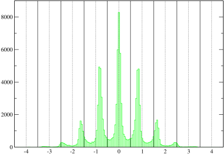
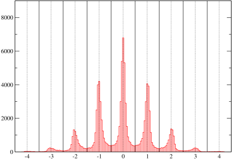
In this paper we investigate the utility of such a renormalized gluonic charge definition for a precision measurement of the topological susceptibility in the pure $SU(3)$ gauge theory. We start from the standard “clover-leaf” definition of $F_{\mu\nu}(x)$ (it uses the average of the antihermitean part of the plaquette $U_{\mu\nu}$ in $x,x\!-\!\hat{\mu},x\!-\!\hat{\nu},x\!-\!\hat{\mu}\!-\!\hat{\nu}$) based on HYP smeared [34] gauge links. Plugging this into (4) we have the bare charge $q_{\mathrm{nai}}[U]$ which is a real number. One of our $q_{\mathrm{nai}}$ distributions ($\beta\!=\!6.0,12^{4}$, 3 HYP steps) is shown in the left panel of Fig. 1. Thanks to CP symmetry only a multiplicative renormalization applies, and we opt for a non-perturbatively defined $Z$-factor. Still, there are various possibilities, and we choose a strategy which makes use of the fact that on fine enough lattices the overall distribution of $q_{\mathrm{nai}}$ tends to cluster near integer values (cf. Fig. 1). We find $Z$ as the solution of

$$\min_{Z>1}(\chi^{2})\qquad\mathrm{where}\qquad\chi^{2}=\sum_{U}\Big{(}Z\,q_{\mathrm{nai}}[U]-\mathrm{round}(Z\,q_{\mathrm{nai}}[U])\Big{)}^{2}$$ (7)

and use it to define, via rounding to the nearest integer, the renormalized field-theoretic charge

$$q_{\mathrm{ren}}[U]=\mathrm{round}(Z\,q_{\mathrm{nai}}[U])$$ (8)

which, by construction, is an integer. This charge definition has already been used in [35].

The alert reader might be surprised by our frequent use of expressions like “we choose” or “we opt for” in this passage. Indeed, there is a huge amount of freedom in how one attributes an integer charge to a lattice configuration. However, according to the standard scaling hypothesis by Symanzik this ambiguity reflects itself in different $O(a^{2})$ cut-off effects of observables built from the topological charge. It has been checked that the “disagreement rate” between any pair of charge definitions quickly vanishes with $\beta\!\to\!\infty$ [37] and that the gluonic or fermionic charge definition yields the same continuum limit for the topological susceptibility [29, 38, 39]. Clearly, this is not a mathematical proof, but it is worth emphasizing that this is exactly the behavior that one expects to see, if one is in the Symanzik scaling regime.

3 Lattice simulations

Our goal is to perform a series of simulations in a fixed physical volume that will allow us to determine the topological charge distribution in the continuum limit (in that volume). This will be complemented by a second series of simulations (at a fixed lattice spacing) to assess possible finite volume effects.

$\beta$	5.8980	6.0000	6.0938	6.1802	6.2602	6.3344
$L/a$	10	12	14	16	18	20
$n_{\mathrm{sepa}}$	10	10	10	50	50	100
$n_{\mathrm{conf}}$	100010	101600	103705	101710	112222	105314
$Z$	1.2902	1.2353	1.1993	1.1742	1.1570	1.1430
$\tau_{\mathrm{int}}(q)$	0.93	2.18	4.83	2.27	4.65	4.61
$\tau_{\mathrm{int}}(q^{2})$	0.61	1.09	2.44	1.19	2.45	2.52
$\tau_{\mathrm{int}}(\mathrm{sign}(q))$	0.89	2.05	4.42	2.10	4.25	4.27
$|\langle q\rangle|$	0.004(5)	0.007(8)	0.007(11)	0.007(8)	0.021(10)	0.010(10)
$\langle q^{2}\rangle$	1.695(9)	1.592(11)	1.490(15)	1.465(10)	1.427(14)	1.381(14)
$\langle q^{4}\rangle/\langle q^{2}\rangle^{2}-3$	0.214(21)	0.238(24)	0.244(27)	0.227(21)	0.241(30)	0.204(32)
$\langle q^{4}\rangle/\langle q^{2}\rangle-3\langle q^{2}\rangle$	0.363(36)	0.378(38)	0.363(40)	0.333(32)	0.344(43)	0.282(44)
$\langle q^{4}\rangle-3\langle q^{2}\rangle^{2}$	0.616(61)	0.602(62)	0.541(60)	0.487(46)	0.490(63)	0.389(61)
$\langle q^{2}\rangle_{q\neq 0}$	1.702(12)	1.610(13)	1.526(22)	1.486(13)	1.461(21)	1.400(19)

Table 1: Summary of the scaling series of runs. Unless stated otherwise, $q$ is the renormalized (i.e. integer) gluonic topological charge $q_{\mathrm{ren}}$ with 3 HYP steps. The subscript “$q\!\neq\!0$” means that the distribution of $|q|$ with $q\!\neq\!0$ has been fitted to a half-Gaussian. Statistical errors have been estimated via a jackknife with the blocklength set to $\mathrm{round}(10\tau_{\mathrm{int}}(q))$.

$\beta$	6.0000	6.0000	6.0000	6.0000	6.0000
$L/a$	10	12	14	16	18
$n_{\mathrm{sepa}}$	10	10	10	10	10
$n_{\mathrm{conf}}$	103600	101600	99000	100000	105000
$Z$	[1.2441]	1.2353	[1.2333]	[1.2332]	[1.2237]
$\tau_{\mathrm{int}}(q)$	1.80	2.18	2.25	2.09	2.13
$\tau_{\mathrm{int}}(q^{2})$	1.34	1.09	1.10	1.11	1.13
$\tau_{\mathrm{int}}(\mathrm{sign}(q))$	1.74	2.05	1.96	1.74	1.71
$|\langle q\rangle|$	0.004(4)	0.007(8)	0.003(11)	0.020(14)	0.023(17)
$\langle q^{2}\rangle$	0.586(5)	1.592(11)	3.012(20)	5.198(34)	8.233(53)
$\langle q^{4}\rangle/\langle q^{2}\rangle^{2}-3$	1.277(41)	0.238(24)	0.095(20)	0.065(19)	0.008(16)
$\langle q^{4}\rangle/\langle q^{2}\rangle-3\langle q^{2}\rangle$	0.748(24)	0.378(38)	0.287(59)	0.338(97)	0.069(139)
$\langle q^{4}\rangle-3\langle q^{2}\rangle^{2}$	0.439(15)	0.602(62)	0.86 (18)	1.76 (50)	0.57 (114)
$\langle q^{2}\rangle_{q\neq 0}$	0.780(10)	1.610(13)	3.009(26)	5.202(51)	8.242(54)

Table 2: Summary of the volume extrapolation series of runs. Throughout, the charge renormalization factors of the ($6.0,12^{4}$) lattices have been used. For details see caption of Tab. 1.

We use the MILC code [40] to produce the $SU(3)$ gauge ensembles. We choose the Wilson gauge action and run parameters as detailed in Tab. 2 (for the scaling series) and Tab. 2 (for the volume extrapolation series). The scale is set via the Sommer radius $r_{0}$ [16], based on a new parameterization of data from [41] as specified in the appendix. The physical value is a separate topic that will be discussed along with the presentation of the final result.

We start with a closer look at Tab. 2. Throughout, our runs are designed to yield $\sim\!10^{5}$ measurements. Anticipating that the autocorrelation time of the topological charge rapidly grows with $\beta$, we have increased the number of updates, $n_{\mathrm{sepa}}$, between adjacent measurements. Still, it turns out that the measured integrated autocorrelation times are somewhat larger on the finer lattices. The renormalization factor $Z$ for $q_{\mathrm{nai}}$ with 3 HYP steps, as defined in (7), seems to go monotonically towards 1 with increasing $\beta$, as expected. Based on it we determine $q\!=\!q_{\mathrm{ren}}$ defined in (8). As a first check, we measure $|\langle q\rangle|$, and this moment is consistent with zero on all lattices. The observable of interest, $\langle q^{2}\rangle$, is measured with 1% statistical accuracy (or better), throughout. We have also checked that using a 2 HYP or 4 HYP charge would change the suscpetibility by an amount which is an order of magnitude smaller than the statistical error of the $\langle q^{2}\rangle$ given. Our data are precise enough to evaluate the fourth moment of the distribution, and the kurtosis $\langle q^{4}\rangle/\langle q^{2}\rangle^{2}-3$ turns out to deviate from zero, for most lattices in the scaling series, by about $10\sigma$. It seems independent of the lattice spacing and it is thus natural to ask whether a non-vanishing $\langle q^{4}\rangle/\langle q^{2}\rangle^{2}-3$ is a finite volume effect.

This brings us to discuss the second series of runs, as detailed in Tab. 2. Potential finite volume effects are commonly attributed to infrared physics; we thus restrict ourselves to a single coupling, $\beta\!=\!6.0$. Again, we aim for $O(10^{5})$ measurements per run. For larger volumes the “crest and valley” structure in Fig. 1 becomes less pronounced, and we pursue the analysis with the $Z$-factor determined on the $(6.0,12^{4}$) lattices. Now one expects the autocorrelation times to be independent of the volume. This happens to be true, except in the $L/a\!=\!10$ case, where we find severe finite volume effects in $\langle q^{2}\rangle$, too (see below). Again $|\langle q\rangle|$ is basically consistent with zero. The second moment $\langle q^{2}\rangle$ is measured, as before, with 1% statistical accuracy (or better) on all lattices. The main point of this series is clear evidence that the kurtosis $\langle q^{4}\rangle/\langle q^{2}\rangle^{2}-3$, which quantifies the deviation from a Gaussian distribution, tends to zero with $V\!\to\!\infty$.

Figure 2: Distribution of $q_{\mathrm{ren}}$ for the $(6.0,12^{4})$ [left] and $(6.3344,20^{4})$ lattices [right]. The fit to a Gaussian form excludes the $q\!=\!0$ sector; the excess gives rise to the kurtosis $\langle q^{4}\rangle/\langle q^{2}\rangle^{2}\!-\!3$ reported in Tab. 1, an effect that goes away in the infinite volume limit, as evident from Tab. 2.

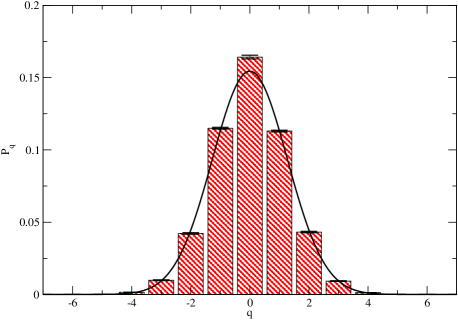
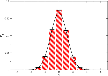
This observation lets us plot the charge histograms for two lattices from the scaling series in Fig. 2. It turns out that the relative weight of the toplogically non-trivial sectors is almost consistent with a Gaussian form, while the $q\!=\!0$ sector shows a clear excess. It is thus tempting to define a new $\langle q^{2}\rangle_{q\neq 0}$ as the width of this Gaussian, where the fit takes only the nontrivial sectors into account. In fact, due to CP symmetry the distribution is even, and we produce a histogram of $|q|$. The $|q|\!\geq\!1$ sectors are then fitted to a half-Gaussian. This procedure stabilizes the contribution from the tails (for this reason a similar “improved estimator” was used in [42]), but it also introduces a model dependence.

4 Continuum and infinite volume extrapolations

$\beta$	6.0000	6.0938	6.1802	6.2602	6.3344
$L/a$	12	14	16	18	20
$\langle q^{2}\rangle(r_{0}/L)^{4}$	6330(60)	5926(71)	5826(57)	5673(67)	5490(66)
$\langle q^{2}\rangle_{q\neq 0}(r_{0}/L)^{4}$	6401(69)	6066(95)	5907(66)	5808(92)	5568(84)

Table 3: Summary of the data from the scaling series of runs, in units of $10^{-5}$. Here, an extra 0.68% error has been added w.r.t. what is reported in Tab. 1.

$L/a\;\;(\beta\!=\!6.0)$	10	12	14	16	18
$\langle q^{2}\rangle(r_{0}/L)^{4}$	4834(42)	6330(42)	6464(43)	6540(43)	6468(42)
$\langle q^{2}\rangle_{q\neq 0}(r_{0}/L)^{4}$	6428(79)	6401(53)	6458(56)	6545(64)	6474(42)

Table 4: Summary of the data from the infinite volume extrapolation series, in units of $10^{-5}$. Here, no extra error has been added w.r.t. what is reported in Tab. 2.

For the continuum and infinite volume extrapolation of the quenched topological susceptibility we convert our data to physical units by multiplying them with the appropriate power of $r_{0}/a$. In the scaling series the uncertainty of $L/r_{0}$ reflects itself independently for each datapoint. Assuming that $L/r_{0}$ is known (at each $\beta$) with 0.17% precision (see Appendix) an extra 0.68% error needs to be included in Tab. 4. By contrast, in the volume extrapolation series the uncertainty of $L/r_{0}$ is correlated, and no extra error has been included in Tab. 4.

Figure 3: Continuum extrapolation of $\chi_{\mathrm{top}}r_{0}^{4}$ in a fixed physical volume, $V=(2.2394r_{0})^{4}$.

Figure 4: Infinite volume extrapolation of $\chi_{\mathrm{top}}r_{0}^{4}$, versus $r_{0}/L$ [cf. (9)] and $(r_{0}/L)^{4}$ [cf. (10)].

Figure 5: Continuum extrapolation of $\langle q^{4}\rangle/\langle q^{2}\rangle^{2}-3$ in a fixed physical volume, $V=(2.2394r_{0})^{4}$.

Figure 6: Left: Infinite volume extrapolation of the kurtosis $\langle q^{4}\rangle/\langle q^{2}\rangle^{2}-3$ in log-log form; this quantity vanishes with $V\!\to\!\infty$. Right: The reduced moment ratio $\langle q^{4}\rangle/\langle q^{2}\rangle-3\langle q^{2}\rangle$ versus $r_{0}^{4}/V$. This plot includes constant fits to the last 2, 3 or 4 datapoints and a linear fit to all 5 points. We cannot discriminate a finite from a vanishing limit of this quantity with $V\!\to\!\infty$.

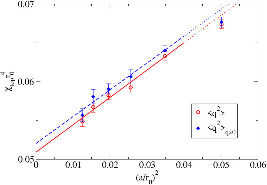
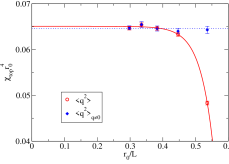
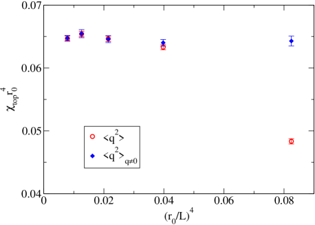
For the continuum extrapolation in a fixed physical volume we plot our data against $(a/r_{0})^{2}$. This power of the lattice spacing is motivated by a Symanzik analysis (both the Wilson action and our topological charge operator contain dimension 6, but no dimension 5 operators). In principle, the uncertainty of $r_{0}/a$ also leads to a horizontal error bar, but its effect is negligible, and we shall omit it. The resulting fits are shown in Fig. 4. The observables $\langle q^{2}\rangle(r_{0}/L)^{4}$ and $\langle q^{2}\rangle_{q\neq 0}(r_{0}/L)^{4}$ extrapolate in a parallel manner, giving the continuum values $0.05092(71)$ and $0.05205(71)$, respectively. The difference, if evaluated inside a jackknife, is significant.

This brings us to the discussion of finite volume effects. Standard reasoning suggests that the dominant finite volume corrections in the YM theory come from glueball states travelling around the box. Since euclidean Green’s functions fall off exponentially, this would imply

$$Z_{\nu}(L)=Z_{\nu}(\infty)\,\Big{(}1+\mathrm{const}\,e^{-M_{G}L}+...\Big{)}$$ (9)

in close analogy to relative finite volume effects in QCD being proportional to $\exp(-M_{\pi}L)$. Simple models for the YM vacuum (random population of unit cells by instantons or anti-instantons) suggest no finite volume corrections for the susceptibility and a $1/V$ type kurtosis. As a result, one may consider the alternative form of the partition function

$$Z_{\nu}(L)=Z_{\nu}(\infty)\,\Big{(}1+\mathrm{const}/L^{4}+...\Big{)}\;.$$ (10)

The data of Tab. 4 are shown in Fig. 4. If we assume exponential finite-volume effects, the data for the first estimator may be fitted all the way out to $L/a\!=\!10$. The difference of the fit curve at $L/a\!=\!12$ and at $L/a\!=\!\infty$ suggests that the continuum result for $\langle q^{2}\rangle(r_{0}/L)^{4}$ is suppressed by the amount $0.00175$, and this gives a corrected $\langle q^{2}\rangle(r_{0}/L)^{4}\!=\!0.05267(71)$. With the other estimator the fitted value for “const” in (9) is consistent with zero, and we stay with $\langle q^{2}\rangle_{q\neq 0}(r_{0}/L)^{4}\!=\!0.05205(71)$, as quoted above. If we assume $1/V$-type effects, finite-volume corrections are hard to quantify (at least the volume-scaling regime with the first estimator is smaller). Therefore, we decide to stay with the extrapolation via (9). Taking the average of both estimators but keeping the full difference as a theoretical uncertainty, we consider

$$\chi_{\mathrm{top}}r_{0}^{4}=0.05236(71)(62)$$ (11)

our final result, where the first error is statistical and the second systematic.

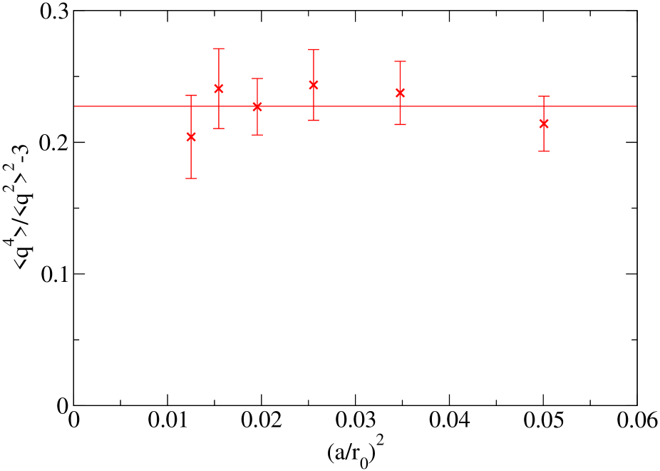
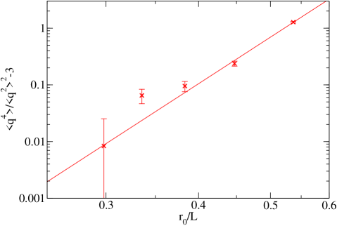
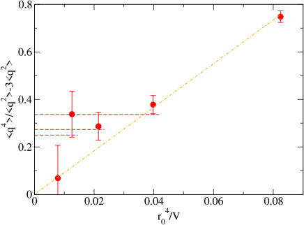
Our data for the kurtosis $\langle q^{4}\rangle/\langle q^{2}\rangle^{2}-3$ scale perfectly (Fig. 6), and the infinite volume extrapolation is consistent with both an exponential and a power law behavior. We find that in the YM theory a non-zero kurtosis is a pure finite volume effect and has nothing to do with the discretization (Fig. 6). Since our “independent cell” model of footnote 7 and large ${N_{\!c}}$ arguments suggest that $\langle q^{4}\rangle/\langle q^{2}\rangle-3\langle q^{2}\rangle$ has a finite limit with $V\!\to\!\infty$, we plot this quantity versus $1/V$ in Fig. 6, too. It turns out that our data are consistent with the value $0.276(84)$ given in [43], but we cannot rule out the possibility that the infinite volume limit might actually vanish.

5 Conversion to physical units

Having an unambiguous result for the topological susceptibility in the combined continuum and infinite volume limit in units of the Sommer scale $r_{0}^{-1}$ [16], we are left with the question which value [in MeV] the latter should be identified with.

In QCD $r_{0}$ is a well-defined quantity. In other words, one could measure $aM_{p}$, $aM_{\pi}$ and $aM_{K}$ in a $2\!+\!1$ flavor simulations in which their ratios are always adjusted to the respective experimental ratios. By considering the continuum limit of $r_{0}M_{p}$, one would have the correct physical value of $r_{0}$, and there is nothing wrong with using this value also in pure YM theory. The original estimate $r_{0}\!=\!0.5\,\mathrm{fm}$ [16] for the outcome of this procedure has been superseded, more recently, by values like $r_{0}\!=\!0.467(6)\,\mathrm{fm}$ [44, 45]. Alternatively, one could set the scale in the quenched theory via $r_{0}f_{K}\!=\!0.4146(94)$ [46], using $f_{K}\!=\!160(2)\,\mathrm{MeV}$ from experiment. This has the same effect as attributing $r_{0}\!=\!0.512(12)\,\mathrm{fm}$. To encompass this spread we set the scale via $r_{0}\!=\!0.49\,\mathrm{fm}$ and add a 4% error to reflect the intrinsic scale ambiguity in pure YM theory.

With this choice for $r_{0}$ our value $\chi_{\mathrm{top}}r_{0}^{4}$, as quoted in the previous section, amounts to

$$\chi_{\mathrm{top}}^{1/4}=193(1)(8)\,\mathrm{MeV}$$ (12)

where the first error bar contains all statistical and systematic uncertainties of our calculation, and the second one reflects the scale setting ambiguity in a theory which is not full QCD.

6 Summary

In this paper we have performed a precision study of the topological susceptibility in pure $SU(3)$ Yang Mills theory in the combined continuum and infinite volume limit using a field-theoretic definition of the topological charge.

	$\;\chi_{\mathrm{top}}r_{0}^{4}$	$\chi_{\mathrm{top}}^{1/4}$ [MeV]	$\chi_{\mathrm{top}}^{1/4}$ [MeV]
Ref. [49] (2001)	0.072(7)	209(5)(8)	—
Ref. [43] (2002)	0.057(3)	197(3)(8)	180(2)(8)
Ref. [39] (2003)	0.055(10)	195(9)(8)	188(12)(8)
Ref. [50] (2003)	0.059(5)	198(4)(8)	—
Ref. [42] (2004)	0.059(3)	198(3)(8)	191(5)(8)
this work	0.0524(9)	193(1)(8)

Table 5: Summary of the quenched topological susceptibility (in the continuum) as determined in some recent studies. The results $\chi_{\mathrm{top}}/\sigma^{2}\!=\!0.0355(33)$ [49] and $\chi_{\mathrm{top}}/\sigma^{2}\!=\!0.0282(12)$ [43] have been converted to $r_{0}^{-4}$ units by means of $\sigma^{1/2}r_{0}=1.193(10)$ [51]. In the second column the conversion to MeV has been done with our choice $r_{0}\!=\!0.49\,\mathrm{fm}$, while the third one contains the values given in the respective papers, but with our standard scale setting error throughout.

Comparing our final result to other recent determinations [49, 43, 39, 50, 42] (see Tab. 5 for details) we see a downward trend over time. Our result in $r_{0}^{-4}$ units is substantially more precise, since we work much closer to the continuum (our $\beta\!=\!6.0$ lattices are the coarsest ones used in the continuum extrapolation) and due to the large statistics. The conversion to $\,\mathrm{MeV}$ is, of course, limited by the basic scale setting ambiguity in the quenched theory. In any case our final result (12) supports the Witten Veneziano scenario for the origin of the $\eta^{\prime}$ mass.

Acknowledgments: We thank Ferenc Niedermayer for useful discussions. Computations were carried out on ALiCEnext and a Pentium4 cluster at the University of Wuppertal. This work was supported by the Swiss NSF and under the Hungarian grant OTKA-AT049652.

Appendix

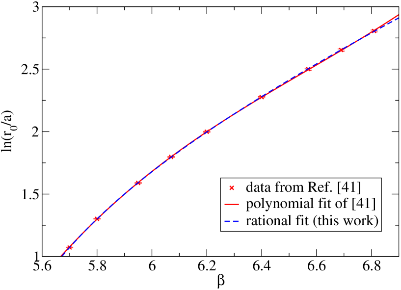
In Ref. [41] Necco and Sommer use a polynomial approximation for $\log(r_{0}/a)$. Specifically

$$\log(r_{0}/a)\Big{|}_{\mathrm{NS}}=c_{0}+c_{1}(\beta-6)+c_{2}(\beta-6)^{2}+c_{3}(\beta-6)^{3}$$ (13)

with $c_{0}\!=\!1.6804,c_{1}\!=\!1.7331,c_{2}\!=\!-0.7849,c_{3}\!=\!0.4428$ is suggested in order to generate matched lattices for $5.7\leq\beta\leq 6.92$, i.e. combinations of $(\beta,L/a)$ with fixed $L/r_{0}$. We have repeated the analysis with their data [41] and find essentially the same $c_{0...3}$, with $\chi^{2}/\mathrm{d.o.f.}=1.39$.

Here, we wish to explore a rational approximation of $\log(r_{0}/a)$ which has the merit of being consistent with perturbation theory. In the weak coupling regime $a\!\propto\!\exp(-1/[2\beta_{0}g_{0}^{2}])$ with the universal coefficient $\beta_{0}\!=\!1/(4\pi)^{2}\cdot[11{N_{\!c}}/3-2{N_{\!f}}/3]$. In $SU(3)$ gluodynamics one has thus $a\!\propto\!\exp(-16\pi^{2}/132\cdot\beta)$ or $\log(r_{0}/a)=4\pi^{2}/33\cdot\beta+...$ and we employ the ansatz

$$\log(r_{0}/a)\Big{|}_{\mathrm{new}}={4\pi^{2}\over 33}\,\beta\cdot{1+d_{1}/\beta+d_{2}/\beta^{2}\over 1+d_{3}/\beta+d_{4}/\beta^{2}}$$ (14)

where this constraint is built in. Using again their data we find that the best fit is given through $d_{1}\!=\!-8.2384,d_{2}\!=\!15.310,d_{3}\!=\!-2.7395,d_{4}\!=\!-11.526$ with $\chi^{2}/\mathrm{d.o.f.}=0.91$.

Figure 7: Old polynomial $\chi^{2}/6\!=\!1.39$ and new rational $\chi^{2}/6\!=\!0.91$ fit to the data of Ref. [41]. Asymptotic freedom demands that the curve eventually becomes linear with slope $4\pi^{2}/33$, and this constraint is built into the new rational ansatz (14).

$L/a$	10	12	14	16	18	20
$\beta$	5.8996	6.0000	6.0926	6.1790	6.2601	6.3362
$L/r_{0}$	2.2357	2.2356	2.2357	2.2357	2.2356	2.2357
$\beta$	5.8980	6.0000	6.0938	6.1802	6.2602	6.3344
$L/r_{0}$	2.2394	2.2394	2.2394	2.2395	2.2393	2.2393

Table 6: Upper part: ($\beta$, $L/a$) combinations which match ($6.0$, $12$) [via achieving $L/r_{0}\!=\!2.2356$ as accurately as possible], based on the interpolation formula (13) of [41]. Lower part: Same [via achieving $L/r_{0}\!=\!2.2394$ as accurately as possible], based on the interpolation formula (14).

It is straightforward to find the $\beta$-values which match a simulation with $(\beta,L/a)=(6.0,12)$. The results are given in Tab. 6, both for (13) and for (14). It turns out that the matched $\beta$-values are more or less the same with either formula and the pertinent $L/r_{0}$ (and hence our estimates for the physical box-length) differ by 0.17% only. This should not come as a surprise, since the two curves in Fig. 7 are rather close. Still, since the new interpolation has a better theoretical foundation and the $\chi^{2}/\mathrm{d.o.f.}$ is lower, we choose the new parameterization (14). Nonetheless, it is clear that the original parametrization (13) remains a legitimate and good one in the interval in which it is given.

References

- [1] H. Leutwyler and A. Smilga, Phys. Rev. D 46, 5607 (1992).
- [2] S. Dürr, Nucl. Phys. B 611, 281 (2001) [hep-lat/0103011].
- [3] G. S. Bali et al. [TXL Collab.], Phys. Rev. D 64, 054502 (2001) [hep-lat/0102002].
- [4] A. Ali Khan et al. [CP-PACS Collab.], Phys. Rev. D 64, 114501 (2001) [hep-lat/0106010].
- [5] A. Hart and M. Teper [UKQCD Collab.], Phys. Lett. B 523, 280 (2001) [hep-lat/0108006].
- [6] T. G. Kovacs, hep-lat/0111021.
- [7] C. Bernard et al. [MILC Collab.], Phys. Rev. D 68, 114501 (2003) [hep-lat/0308019].
- [8] T. A. DeGrand and S. Schaefer, Phys. Rev. D 72, 054503 (2005) [hep-lat/0506021].
- [9] G. I. Egri, Z. Fodor, S. D. Katz and K. K. Szabo, JHEP 0601, 049 (2006) [hep-lat/0510117].
- [10] A. Hasenfratz and R. Hoffmann, Phys. Rev. D 74, 114509 (2006) [hep-lat/0609067].
- [11] E. Witten, Nucl. Phys. B 156, 269 (1979).
- [12] G. Veneziano, Nucl. Phys. B 159, 213 (1979).
- [13] P. Minkowski, Phys. Lett. B 237, 531 (1990).
- [14] P. Minkowski, Phys. Lett. B 423, 157 (1998) [hep-ph/9711431].
- [15] L. Girlanda, J. Stern and P. Talavera, Phys. Rev. Lett. 86, 5858 (2001) [hep-ph/0103221].
- [16] R. Sommer, Nucl. Phys. B 411, 839 (1994) [hep-lat/9310022].
- [17] M. F. Atiyah and I. M. Singer, Annals Math. 87, 484 (1968).
- [18] M. Lüscher, Commun. Math. Phys. 85, 39 (1982).
- [19] A. Phillips and D. Stone, Commun. Math. Phys. 103, 599 (1986).
- [20] T. A. DeGrand [MILC Collab.], Phys. Rev. D 63, 034503 (2001) [hep-lat/0007046].
- [21] W. Bietenholz, hep-lat/0611030.
- [22] H. Neuberger, Phys. Lett. B 417, 141 (1998) [hep-lat/9707022].
- [23] P. H. Ginsparg and K. G. Wilson, Phys. Rev. D 25, 2649 (1982).
- [24] P. Hasenfratz, V. Laliena and F. Niedermayer, Phys. Lett. B 427, 125 (1998) [hep-lat/9801021].
- [25] M. Lüscher, Phys. Lett. B 428, 342 (1998) [hep-lat/9802011].
- [26] M. Göckeler, A. S. Kronfeld, M. L. Laursen, G. Schierholz and U. J. Wiese, Phys. Lett. B 233, 192 (1989).
- [27] M. Campostrini, A. Di Giacomo, H. Panagopoulos and E. Vicari, Nucl. Phys. B 329, 683 (1990).
- [28] A. Di Giacomo and E. Vicari, Phys. Lett. B 275, 429 (1992).
- [29] B. Alles, M. D’Elia, A. Di Giacomo and R. Kirchner, Phys. Rev. D 58, 114506 (1998) [hep-lat/9711026].
- [30] E. Seiler and I. O. Stamatescu, MPI-PAE/PTH10/87.
- [31] S. Chandrasekharan, Phys. Rev. D 60, 074503 (1999) [hep-lat/9805015].
- [32] F. Niedermayer, Nucl. Phys. Proc. Suppl. 73, 105 (1999) [hep-lat/9810026].
- [33] L. Giusti, G. C. Rossi and M. Testa, Phys. Lett. B 587, 157 (2004) [hep-lat/0402027].
- [34] A. Hasenfratz and F. Knechtli, Phys. Rev. D 64, 034504 (2001) [hep-lat/0103029].
- [35] S. Dürr, Comput. Phys. Commun. 172, 163 (2005) [hep-lat/0409141].
- [36] C. Christou, A. Di Giacomo, H. Panagopoulos and E. Vicari, Phys. Rev. D 53, 2619 (1996) [hep-lat/9510023].
- [37] C. R. Gattringer, I. Hip and C. B. Lang, Nucl. Phys. B 508, 329 (1997) [hep-lat/9707011].
- [38] N. Cundy, M. Teper and U. Wenger, Phys. Rev. D 66, 094505 (2002) [hep-lat/0203030].
- [39] L. Del Debbio and C. Pica, JHEP 0402, 003 (2004) [hep-lat/0309145].
- [40] http://www.physics.utah.edu/detar/milc
- [41] S. Necco and R. Sommer, Nucl. Phys. B 622, 328 (2002) [hep-lat/0108008].
- [42] L. Del Debbio, L. Giusti and C. Pica, Phys. Rev. Lett. 94, 032003 (2005) [hep-th/0407052].
- [43] L. Del Debbio, H. Panagopoulos and E. Vicari, JHEP 0208, 044 (2002) [hep-th/0204125].
- [44] A. A. Khan et al. [QCDSF Collab.], hep-lat/0603028.
- [45] C. Aubin et al. [MILC Collab.], Phys. Rev. D 70, 094505 (2004) [hep-lat/0402030].
- [46] J. Garden, J. Heitger, R. Sommer and H. Wittig [ALPHA Collaboration], Nucl. Phys. B 571, 237 (2000) [hep-lat/9906013].
- [47] C. Gattringer, R. Hoffmann and S. Schaefer, Phys. Lett. B 535, 358 (2002) [hep-lat/0203013].
- [48] P. Hasenfratz, S. Hauswirth, T. Jörg, F. Niedermayer and K. Holland, Nucl. Phys. B 643, 280 (2002) [hep-lat/0205010].
- [49] B. Lucini and M. Teper, JHEP 0106, 050 (2001) [hep-lat/0103027].
- [50] L. Giusti, M. Lüscher, P. Weisz and H. Wittig, JHEP 0311, 023 (2003) [hep-lat/0309189].
- [51] F. Niedermayer, P. Rüfenacht and U. Wenger, Nucl. Phys. B 597, 413 (2001) [hep-lat/0007007].
- [52] L. Giusti, B. Taglienti, S. Petrarca, PoS(LAT2006) 058.