Analytic continuation from imaginary to real chemical potential in two-color QCD

Abstract:

The method of analytic continuation from imaginary to real chemical potential is one of the most powerful tools to circumvent the sign problem in lattice QCD. Here we test this method in a theory, two-color QCD, which is free from the sign problem. We find that the method gives reliable results, within appropriate ranges of the chemical potential, and that a considerable improvement can be achieved if suitable functions are used to interpolate data with imaginary chemical potential.

1 Introduction

The phase diagram of QCD in the temperature – chemical potential plane is the subject of many present investigations. Understanding the different phases and the transitions among them has strong implications in cosmology, in astrophysics and in the phenomenology of heavy ion collisions. Unfortunately, perturbation theory and approaches based on effective models can handle a limited number of issues of the QCD phase diagram and, in fact, the lattice formulation is the only tool for a quantitative approach to the problem based on first principles. For non-zero chemical potential, however, the QCD fermion determinant becomes complex and the probability interpretation of the QCD Euclidean action, necessary for the standard Monte Carlo importance sampling, is lost, this being the well-known “sign problem”.

Several methods have been invented to circumvent this problem (for a review, see [1] and [2]): the reweighting from the ensemble at $\mu=0$ [3, 4, 5, 6], the Taylor expansion method [7, 8, 9, 10, 11, 12, 13, 14, 15], the canonical approach [16, 17, 18, 19], the density of states method [20, 21, 22, 23, 24, 25, 26] and the method of analytic continuation from an imaginary chemical potential [27, 28, 29, 30, 31, 32, 33, 34, 35, 36, 37, 38, 39, 40, 41, 42, 43, 44, 45, 46, 47, 48]. Their application has allowed to get relevant information on the critical line separating the hadronic phase from the quark-gluon plasma phase in the region $\mu/T\lesssim 1$.

In this paper we focus our attention on the method of analytic continuation. The idea behind this method is very simple: numerical simulations are performed at imaginary chemical potential, $\mu=i\mu_{I}$, for which the fermion determinant is real, then Monte Carlo determinations are interpolated by a suitable function and finally this function is analytically continued to real values of $\mu$. This method is rather powerful since the coupling $\beta$ and the chemical potential $\mu$ can be varied independently and there is no limitation from increasing lattice size, as happens with other methods, like those based on reweighting. There is, however, an important drawback: the periodicity of the QCD partition function and the presence of non-analyticities arising for imaginary values of the chemical potential [49] restrict the region useful for numerical determinations to the strip $0\leq\mu_{I}/T<\pi/3$, or even less in presence of “physical” phase transitions. This implies that the accuracy in the interpolation of the results at imaginary chemical potential has a strong impact on the extension of the domain of real $\mu$ values reachable after analytic continuation. In that sense it is very important to answer the question about which is the optimal way to extract information from data at imaginary chemical potential, i.e. which is the best choice for the interpolating function, which only in a some cases can be guided by physical intuition, leading to some particular prediction for the behaviour at real $\mu$. Moreover one should always be careful about the actual ranges of applicability of the method, which can be influenced by the various physical and unphysical transitions present in the QCD phase diagram, leading to possible non-analyticities.

So far, the method of analytic continuation has been applied in SU(3) with $n_{f}=2$ [29, 30], $n_{f}=3$ [31, 32] and $n_{f}=4$ [33, 34, 35, 43]. Moreover, it has been tested in several theories which do not suffer from the sign problem, by direct comparison of the analytic continuation with Monte Carlo results obtained at real $\mu$ [28, 36, 37, 44]. In most of these applications, a truncated Taylor series (or, more simply, a polynomial) has been used as interpolating function, sometimes a Fourier sum for the low temperature region [33, 34].

The aim of this paper is to study limitations and possible improvements of the method of analytic continuation, by considering its application to SU(2) or two-color QCD. This theory is free from the sign problem and Monte Carlo numerical simulations at real values of the chemical potential are feasible. This allows to compare the extrapolations from imaginary to real chemical potential with direct determinations allowing at the same time both to discriminate among different Ansätze for the interpolating functions and to directly test the range of reliability of the method itself. The experience gained in this way can then be hopefully used as a guide in applications to the real theory.

Figure 1: (Left) Phase diagram in the $(T,\theta)$ plane according to Ref. [49]. (Right) Tentative phase diagram in the $(T,\theta)$ plane after the inclusion of the chiral critical lines.

Figure 2: Phase diagram in the $(\beta,\hat{\mu}_{I})$-plane; $N$ is the number of colors, $N_{\tau}$ the extension of the lattice in the temporal direction. The numerical values for $\beta_{E}$ and $\beta_{c}$ are valid for SU(2) in presence of $n_{f}=8$ degenerate staggered fermions with mass $am=0.07$.

The paper is organized as follows: in Section 2, we briefly recall some general properties of the phase diagram of SU(N) gauge theories in the temperature - imaginary chemical potential plane and discuss their implications on the method of analytic continuation; in Section 3, we present our numerical results and discuss both the choice of the best interpolating function, showing that functions different from polynomials can considerably improve the method, and the ranges where analytic continuation is reliable; finally, in Section 4, we draw our conclusions.

2 Theoretical background

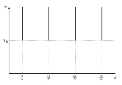
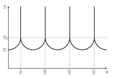
Long ago Roberge and Weiss (RW) have shown [49] that the partition function of any SU(N) gauge theory with non-zero temperature and imaginary chemical potential, $\mu=i\mu_{I}$, is periodic in $\theta\equiv\mu_{I}/T$ with period $2\pi/N$ and that the free energy $F$ is a regular function of $\theta$ for $T<T_{E}$, while it is discontinuous at $\theta=2\pi(k+1/2)/N$, $k=0,1,2,\ldots$, for $T>T_{E}$, where $T_{E}$ is a characteristic temperature, depending on the theory. The resulting phase diagram in the $(T,\theta)$-plane is given in Fig. 1 (left), where the vertical lines represent first order transition lines. This structure is compatible with the $\mu\to-\mu$ symmetry, related with CP invariance, and with the Roberge-Weiss periodicity. The $\mu_{I}$-dependence of any observable is completely determined if this observable is known in the strip $0\leq\theta<\pi/N$. It may be useful to recall the two steps in the proof of periodicity in SU(N): first, the phase transformation

$$\psi(\vec{x},\tau)\longrightarrow\exp(i\tau\mu_{I})\psi(\vec{x},\tau)\;,$$ (1)

then a gauge transformation with periodicity up to an element of the center group Z(N), i.e. a transformation with gauge group elements $U(\vec{x},\tau)$ satisfying the boundary condition

$$U(\vec{x},aN_{\tau})=\exp(2\pi ik/N)U(\vec{x},0)\;,\;\;\;\;\;k\mbox{ integer}\;,$$ (2)

where $N_{\tau}$ is the lattice size in the temporal direction and $a$ is the lattice spacing. The RW periodicity of the partition function extends to the observables which are left unchanged by these two transformations. This is certainly the case of the chiral condensate $\langle\bar{\psi}\psi\rangle$. The Polyakov loop $L\equiv\prod_{\tau=1,N_{\tau}}U(\vec{x},a\tau)$, instead, takes the factor $\exp(2\pi ik/N)$ under the transformation (2), which implies that $\langle L\rangle$ moves, continuously or discontinuously according to the temperature, from one Z(N) sector to the other when $\mu_{I}$ passes from one RW sector to the next. As a consequence, the chiral condensate has the same periodicity in $\mu_{I}/T$ of the partition function, $2\pi/N$, while $\langle L\rangle$ has periodicity in $\mu_{I}/T$ equal to $2\pi$. These predictions have been confirmed numerically in several cases [29, 30, 33, 34, 35, 36, 37].

A phase diagram like that in Fig. 1 (left) would imply the absence of any transition along the $T$ axis in the physical regime of zero chemical potential for any value of $N$, $n_{f}$ and the quark masses, which cannot be true. Therefore, it is necessary to admit that the phase diagram in the $(T,\theta)$-plane is more complicated than in Fig. 1 (left). The simplest possibility is given in Fig. 1 (right), where the added lines generally represent transitions which can be first order, second order or crossover, and can be considered as the continuation of the physical critical line taking place for real chemical potentials. The temperature $T_{c}$ is the critical or pseudo-critical one for the transition at zero chemical potential. The temperature $T_{E}$ represents the endpoint of the RW transition lines: the fact that the continuation of the physical critical line ends right on $T_{E}$ is not expected a priori, but is the result of numerical investigations [29, 30, 33, 34, 35].

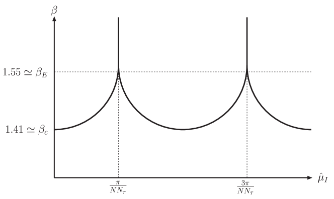
It is convenient to redraw the phase diagram of Fig. 1 (right) in the $(\beta,\hat{\mu}_{I})$-plane (Fig. 2), where $\beta=2N/g^{2}$, $\hat{\mu}_{I}\equiv a\mu_{I}$ is the imaginary chemical potential in lattice units and it has been used the fact that $T=1/(aN_{\tau})$.

Given this phase diagram, it is possible to distinguish three different regimes, corresponding to different ranges of temperature (i.e. of $\beta$), where analytic continuation can apply differently.

Regime a: $T>T_{E}$ (or $\beta>\beta_{E}$).

This regime corresponds to temperatures for which the only expected non-analyticity at imaginary chemical potential is represented by the RW transition line. In this case the useful interval in $\hat{\mu}_{I}$ for numerical simulations is $[0,\pi/8]$. On the side of the real chemical potential, no transition line is expected. This situation is, in some sense, the best possible for the application of the method of analytic continuation. Simulations at imaginary $\mu$ can be done on a relatively large interval and, if the optimal interpolating function is found, its continuation should reproduce data for any real value of $\mu$. The last expectation could actually be wrong if the critical behaviour induced by the RW line had some influence on the ranges of analyticity for the partition function also for real values of the chemical potential: this is an important point that can be directly checked in two-color QCD.

Regime b: $T_{c}<T<T_{E}$ (or $\beta_{c}<\beta<\beta_{E}$).

This regime corresponds to temperatures for which a non-analyticity is expected at a $\hat{\mu}_{I}$ value smaller than $\pi/8$. On the side of the real chemical potential, no transition line is expected. This situation is similar to the previous, with the important difference that the useful interval in $\hat{\mu}_{I}$ for numerical simulations is restricted and the critical behaviour induced by the transition line may be different, thus making in practice more difficult to find the optimal interpolation.

Regime c: $T<T_{c}$ (or $\beta<\beta_{c}$).

This regime corresponds to temperatures for which no non-analyticities should be met in $\hat{\mu}_{I}$. This implies that $\hat{\mu}_{I}$ can be varied at will, although no additional information for the observables of interest here can be gotten by going farther than $\hat{\mu}_{I}=\pi/4$, owing to the RW periodicity. This regime of temperatures is probably the most interesting for physics, since a transition is expected here for a certain real value of the chemical potential. This implies that, no matter how good is the interpolation of data at imaginary chemical potential, its continuation to real $\mu$ should fail to reproduce data above a certain value.

Figure 3: Negative side of the horizontal axis: imaginary part of the fermionic number density vs. the imaginary chemical potential at $\beta=1.90$. Positive side of the horizontal axis: real part of the fermionic number density vs. the real chemical potential at $\beta=1.90$. The green (blue) solid line represents the polynomial (ratio of polynomials) interpolating function; the dashed lines give the corresponding uncertainty, coming from the errors in the parameters of the fit.

Figure 4: Chiral condensate vs. $\mu^{2}$ at $\beta=1.90$. The green (blue) solid line represents the polynomial (ratio of polynomials) interpolating function; the dashed lines give the corresponding uncertainty, coming from the errors in the parameters of the fit.

Figure 5: As in Fig. 4 for the Polyakov loop.

Figure 6: $\chi^{2}$/d.o.f. of the global fit to real and imaginary chemical potential data for the Polyakov loop at $\beta=1.90$, for various fitting functions, as the maximum value $\mu_{\rm max}$ of real chemical potential taken into account is varied. Lines connecting data point have been drawn to guide the eye.

3 Numerical results

We have performed numerical simulations on a $16^{3}\times 4$ lattice of the SU(2) gauge theory with $n_{f}=8$ degenerate staggered fermions having mass $am=0.07$. For this theory the tentative phase diagram looks like in Fig. 2, with $\beta_{E}\simeq 1.55$ [36, 37] and $\beta_{c}\simeq 1.41$ [50]. The algorithm adopted has been the usual exact $\phi$ algorithm described in Ref. [51], properly modified for the inclusion of a finite chemical potential by multiplying the forward (backward) temporal part of the Dirac matrix by $e^{\hat{\mu}}$ ($e^{-\hat{\mu}}$), for the case of a real chemical potential, and by $e^{i\hat{\mu}_{I}}$ ($e^{-i\hat{\mu}_{I}}$) for the case of an imaginary chemical potential. In particular that implies, for real chemical potentials, the impossibility of exploiting the usual even-odd factorization trick for reducing the number of flavors from 8 to 4. The choice of 8 flavors is therefore linked to the need of using an exact Hybrid Monte Carlo algorithm: the last is an unavoidable requirement if we want to make a detailed comparison of data at imaginary values of $\mu$ with data at real values of $\mu$, since systematic effects due to an inexact algorithm could be different for the two cases. The choice of a large volume is instead essential if we want to make a careful test of the method of analytic continuation, since possible non-analyticities will show up only in the thermodynamic limit. The observables we determined are the Polyakov loop, the chiral condensate and the fermionic number density $\langle n_{q}\rangle$.

Figure 7: As in Fig. 3 for $\beta=1.45$.

Figure 8: As in Fig. 4 for $\beta=1.45$.

Figure 9: As in Fig. 5 for $\beta=1.45$.

Figure 10: As in Fig. 6 for $\beta=1.45$.

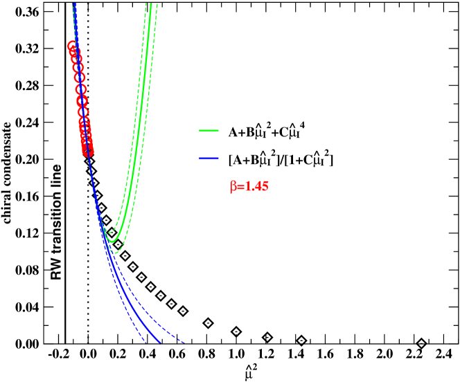
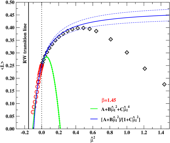
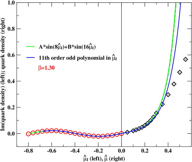
We have considered three $\beta$ values, $\beta$=1.90, 1.45 and 1.30, corresponding to the three different regimes exposed in Section 2, and for each we have taken measurements for several values of the chemical potential, both imaginary and real. The summary of numerical simulations is given in Tables 1, 2, 3, 4, 5, 6. Simulations have been performed on the APE100 and APEmille crates in Bari and on the recently installed computer facilities at the INFN apeNEXT Computing Center in Rome. Statistics have been chosen so as to have statistical errors well below 1% in most cases: indeed our ability to discern the best among a set of possible interpolating functions as well as to detect the exact ranges beyond which analytic continuation fails, is strictly related to the statistical precision of our data.

We have chosen two different strategies for our analysis. We have used the data at imaginary chemical potential $\mu_{I}$ to determine the parameters of the interpolating function, then we have analytically continued this function to real values of the chemical potential and compared there with direct Monte Carlo determinations. In this way we are able to test how the method of analytic continuation is able to reproduce the correct physical results for real values of $\mu$, and to understand which is the best suited function to do so.

As an alternative way to analyze our results, we have tried to fit both sets of data together, at imaginary and real chemical potential, with several analytic functions and using variable ranges for both $\hat{\mu}$ and $\hat{\mu}_{I}$. In this way, using the $\chi^{2}$ test as a statistical tool, we are able to understand in which ranges, if any, the method of analytic continuation makes any sense at all, at least within the set of analytic functions taken into considerations.

In order to fulfill CP invariance, the interpolating function must be a even function of $\mu$ for observables, such as the Polyakov loop and the chiral condensate, which do not depend explicitly on $\mu$. The fermionic number density, being the logarithmic derivative of the partition function with respect to the chemical potential, is instead an odd function of $\mu$.

Figure 11: Negative side of the horizontal axis: imaginary part of the fermionic number density vs. the imaginary chemical potential at $\beta=1.30$. Positive side of the horizontal axis: real part of the fermionic number density vs. the real chemical potential at $\beta=1.30$. The green (blue) solid line represents the Fourier (polynomial) interpolating function and its continuation; the dashed lines give the corresponding uncertainty, coming from the errors in the parameters of the fit.

Figure 12: Chiral condensate vs. $\mu^{2}$ at $\beta=1.30$. The green (blue) solid line represents the Fourier (polynomial) interpolating function and its continuation; the dashed lines give the corresponding uncertainty, coming from the errors in the parameters of the fit.

Figure 13: As in Fig. 12 for the Polyakov loop.

Figure 14: $\chi^{2}$/d.o.f. of the global fit to real and imaginary chemical potential data for the various observable at $\beta=1.30$, as a function of the maximum value $\mu_{\rm max}$ of real chemical potential taken into account. Fitting functions are the same used for Figs. 11, 12, 13 and reported in Eq. (7), (8) and (9). The values of $\chi^{2}$/d.o.f. are quite stable around one for all observables, till $\hat{\mu}_{\rm max}$ crosses the pseudo-critical point.

Figure 15: Susceptibility of the chiral condensate at $\beta=1.30$ for real $\hat{\mu}$.

We separate the discussion of our results for the three different regimes, reflecting the different strategies followed in searching for the optimal interpolation and the different behaviors observed for the physical observables.

3.1 The high temperature region $\beta>\beta_{E}$

For this region we have used two kinds of interpolating functions for the data at imaginary $\mu$: polynomials and ratio of polynomials, the last choice being related to the use of Padé approximants suggested in Ref. [45]. For the Polyakov loop and the chiral condensate we have considered a second order polynomial in $\mu^{2}$,

$$A+B\hat{\mu}_{I}^{2}+C\hat{\mu}_{I}^{4}\;,$$ (3)

according to the standard approach, and the ratio of two first order polynomials in $\mu^{2}$,

$$\frac{A+B\hat{\mu}_{I}^{2}}{1+C\hat{\mu}_{I}^{2}}\;,$$ (4)

according to our new proposal. Similarly, for the fermionic number density we have used a polynomial of the form

$$A\hat{\mu}_{I}+B\hat{\mu}_{I}^{3}+C\hat{\mu}_{I}^{5}\;,$$ (5)

and the ratio

$$\frac{A\hat{\mu}_{I}+B\hat{\mu}_{I}^{3}}{1+C\hat{\mu}_{I}^{2}}\;.$$ (6)

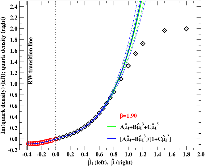
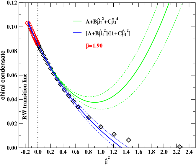
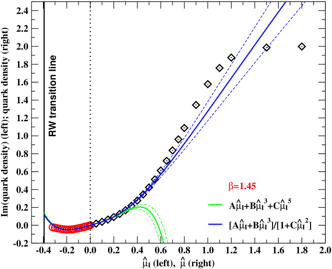
Our findings at $\beta=1.90$ are summarized in Figs. 3, 4, 5 and Table 7. In Fig. 3 we put on the same plot the imaginary part of the fermionic number density as a function of $\mu_{I}$ and the real part of the fermionic number density as a function of the real $\mu$. The two data sets match smoothly at $\mu=0$, which is a necessary condition for the applicability of the method of analytic continuation. The fermionic density approaches two for large values of the real chemical potential. This saturation effect is a lattice artifact, which is due to the fact that no more than two fermions per site can be accommodated on the lattice (“Pauli blocking”), and manifests itself for values of the chemical potential which are close to the ultraviolet cutoff, i.e. for $\hat{\mu}$ of order 1 (see Refs.[52, 53] for a recent discussion of this phenomenon). The solid lines represent the two kinds of interpolating functions, whose parameters are determined by a fit on the data at imaginary chemical potential. Here both interpolations, polynomial and rational function, nicely reproduce the data at real $\mu$ over a large interval. Deviations start at values of $\mu$ for which the saturation effects are certainly important.

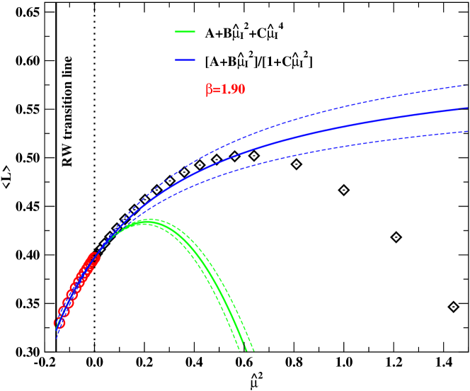
In Fig. 4 we show the chiral condensate as a function of $\mu^{2}$. Again data at imaginary $\mu$, i.e. $\mu^{2}<0$, and data at real $\mu$, i.e. $\mu^{2}>0$, nicely match at $\mu=0$. This time the different behavior of the two kinds of interpolation clearly emerges. The ratio of first order polynomials in $\mu^{2}$ reproduces the data at real $\mu$ on a much larger interval than the second order polynomial in $\mu^{2}$. Deviations arise for values of real $\mu$ for which saturation effects are probably already important. The same conclusions can be drawn from Fig. 5 which shows data and interpolations for the Polyakov loop.

The above conclusions do not change if larger order terms are included in the polynomial interpolation (3). In fact, larger order polynomials fail to reproduce the data at real $\mu$ even earlier in $\mu$ than second order polynomials. This is due to the fact that the higher order terms of the polynomial are the less accurately determined in the fit to data at imaginary $\mu$. On the other side, if in the ratio of polynomials the order of the polynomials at the numerator and/or at the denominator is increased, no improvement is observed.

It is interesting to compare the parameters in the expansion (5) with those predicted by the perturbation theory in $\mu/T$ of the fermionic density. In the infinite temperature limit, and taking into account the rotation to real chemical potential in Eq. (5), it should be $A=-n_{f}/N_{\tau}^{2}=-1/2$ and $B=n_{f}/\pi^{2}=8/\pi^{2}=0.810569...$ [13]. These values are in rough agreement with our findings at the largest available $\beta$ (see Table 7).

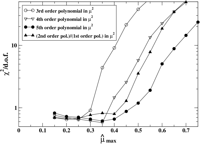
We now expose the results of our combined fits using both sets of data at imaginary and real values of $\mu$. The range of values used in the fit is limited on the imaginary chemical potential side by the presence of the RW transition, so that we included all data with $\hat{\mu}_{I}<\pi/8$. For real chemical potentials, we have considered the possible presence of non-analyticities and have repeated our fits for different values of the maximum real chemical potential, $\hat{\mu}_{\rm max}$.

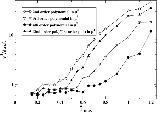
We report only results obtained for the Polyakov loop: those obtained for the other two observables look very similar. We have tried fits with several analytic functions, only a few of them being exemplified in Fig. 6, where we report the value of $\chi^{2}$/d.o.f. as a function of $\hat{\mu}_{\rm max}$. The outcome of our analysis, as evident from Fig. 6, can be summarized as follows: acceptable values of $\chi^{2}$/d.o.f. are obtained once sufficiently higher order polynomials or ratio of polynomials are taken into account, but only if $\hat{\mu}_{\rm max}$ is less than about 0.5. Instead the value of $\chi^{2}$/d.o.f. gets sensibly different from one for larger values of $\hat{\mu}_{\rm max}\to 1$, regardless of the interpolating function.

We interpret this result as a proof that, within statistical errors, data at real and imaginary chemical potential can indeed be described by one only analytic function, even if in a limited range. Hints of possible non-analyticities appear for real chemical potentials $\hat{\mu}>0.5$. We believe that the most plausible explanation of them is the onset of saturation effects.

A comment is in order about the use of higher order polynomials. Fig. 6 could give the impression that increasing the order of the polynomial sensibly improves the method of analytic continuation, since a reasonable $\chi^{2}$/d.o.f. is obtained for a wider range. This could seem to contradict our previous statements about the choice of the optimal function for extrapolating data from imaginary values of $\mu$, in fact it is not so. Indeed, one should consider that when trying to extrapolate information to $\mu^{2}>0$ having at disposal only information from negative values of $\mu^{2}$, the use of polynomials in $\mu^{2}$ can result in instabilities in the determination of the coefficients, since a polynomial with positive coefficients for $\mu^{2}<0$ is continued to a polynomial with alternating coefficients for $\mu^{2}>0$ and vice versa. These instabilities clearly disappear if data on both sides are available, but of course this situation cannot be reproduced for real QCD.

3.2 The intermediate region $\beta_{c}<\beta<\beta_{E}$

Our findings at $\beta=1.45$ are summarized in Figs. 7, 8, 9 and Table 8. Also in this case we have used polynomials and ratio of polynomials as interpolating functions for the data at imaginary $\mu$. Here the discussion goes along the same lines as for $\beta=1.90$ with one important difference: both in the case of polynomials or ratios of polynomials as interpolating functions, and for any of the three observables considered here, a fit at imaginary chemical potential with $\chi^{2}$/d.o.f of the order of one is possible only in the interval $[0,\bar{\mu}_{I}]$, with $\bar{\mu}_{I}=0.22\div 0.24$. This $\hat{\mu}_{I}$ represents the onset of a transition, which shows up also as a peak in the chiral condensate susceptibility, centered around that value of $\hat{\mu}_{I}$. The fact that the interval in $\hat{\mu}_{I}$ available for numerical simulations is shorter makes the interpolation, and consequently its continuation, less accurate. Nevertheless, also at this $\beta$, the use of ratio of polynomial performs much better than simple polynomials.

Also in this regime we have performed combined fits using both sets of data at imaginary and real values of $\mu$. In this case the range of values used in the fit is limited, on the imaginary chemical potential side, by the presence of the continuation of the physical critical line, so that we have included only values $\hat{\mu}_{I}<0.20$.

Also in this case we report only results obtained for the Polyakov loop with several fitting functions, as exemplified in Fig. 10, as a function of $\hat{\mu}_{\rm max}$. Results look very similar to those obtained for $\beta=1.90$, with a few differences: while the quality of the fits obtained with the ratio of polynomials does not change with respect to $\beta=1.90$, higher order polynomials are necessary to obtain reasonable $\chi^{2}$/d.o.f., and hints of non-analyticities show up generally earlier, as a function of $\hat{\mu}_{\rm max}$, than for $\beta=1.90$. A possible explanation for the different behaviour could reside in the presence of the physical pseudo-critical line for imaginary values of $\mu$.

3.3 The low temperature region $\beta<\beta_{c}$

Below $\beta_{c}$ our observables are smooth functions of $\hat{\mu}_{I}$, with periodicity in $\hat{\mu}_{I}$ equal to $\pi/4$ in the case of the fermionic number density and of the chiral condensate and equal to $\pi/2$ in the case of the Polyakov loop. This leads naturally to the use of Fourier sums as interpolating functions and, in particular,

$$A+B\cos(8\hat{\mu}_{I})+C\cos(16\hat{\mu}_{I})$$ (7)

for the chiral condensate,

$$A\cos(4\hat{\mu}_{I})+B\cos(12\hat{\mu}_{I})$$ (8)

for the Polyakov loop and

$$A\sin(8\hat{\mu}_{I})+B\sin(16\hat{\mu}_{I})$$ (9)

for the fermionic number density, which is odd in $\mu_{I}$.

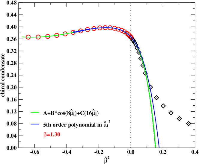
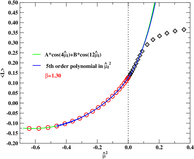
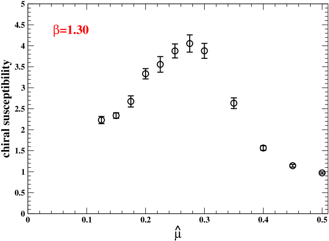
We summarize our results at $\beta=1.30$ in Figs. 11, 12, 13 and Table 9. The functions chosen for our fits, and reported in Eq. (7), (8) and (9), are those containing the minimum number of terms necessary to obtain a $\chi^{2}$/d.o.f. close to one (the use of less terms leading to a sensible increase of $\chi^{2}$/d.o.f.). From Table 9 it is possible to see that the coefficients of the secondary harmonic terms in the Fourier sums (7), (8) and (9) are suppressed by a factor of a few tens with respect to the coefficients of the dominant harmonic, thus signaling a quite fast convergence of the Fourier sums. It is interesting to notice that the term proportional to $\cos(8\hat{\mu}_{I})$ does not appear in Eq. (8), i.e. one term in the harmonic series for the Polyakov loop seems to be missing. The reason is that in the low temperature region center symmetry constrains the Polyakov loop to be zero at $\hat{\mu}_{I}=\pi/8$ (corresponding to the border between the two center sectors), so that all frequencies which are even multiples of $4\hat{\mu}_{I}$ must be excluded. We have verified that if these frequencies are included in the interpolating function, the corresponding coefficients are put to zero by the fit. The Fourier sums become sums of hyperbolic sine and cosine functions after continuation to real $\mu$, which diverge very rapidly and reproduce only partially the data at real $\mu$. The deviation between the extrapolation and the data can be taken as an estimate of the pseudo-critical value of $\hat{\mu}_{R}$. This is confirmed by the study of the chiral condensate susceptibility, which exhibits a peak centered around that value.

Alternative attempts with longer Fourier sums or with ratios of Fourier sums did not change this scenario. In the case of polynomials as interpolating functions, the behavior is similar to Fourier sums if, however, large order polynomials are used (see blue lines in Figs. 11, 12, 13). In this case, the interpolation of data at imaginary $\mu$ works in an interval shorter than that for Fourier sums. These observations confirm that Fourier sums are indeed the natural functions to be used for the analytic continuation in the low temperature region.

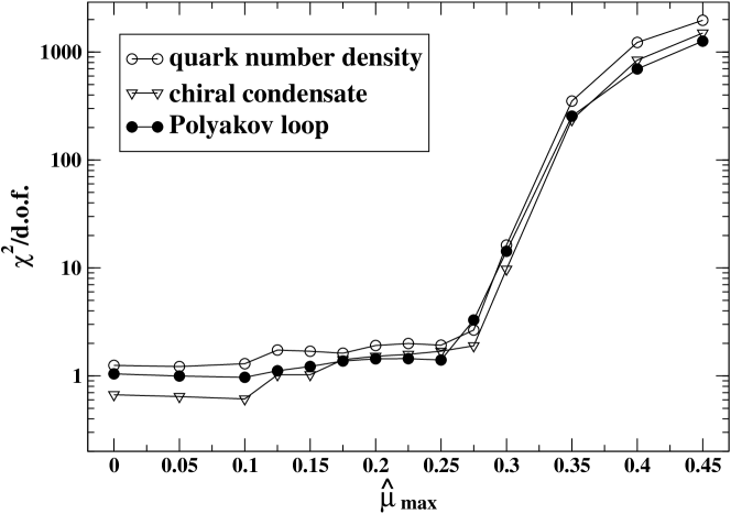
Regarding the global combined fits using both sets of data at imaginary and real values of $\mu$, the results of our analysis are reported in Fig. 14. In this case we report results for all observables, with the same fitting functions, Eq. (7), (8) and (9), used previously. All data at imaginary chemical potential are taken into account, since no phase transition at all is expected on that side, while data at real $\mu$ are limited to a maximum value $\hat{\mu}_{\rm max}$. It clearly emerges that, for all observables, both sets of data can be nicely fitted by a common analytic function, till $\hat{\mu}_{\rm max}$ reaches the region where the physical pseudo-critical point is located; at that point the method of analytic continuation clearly loses any sense. However, it is quite interesting to notice that the analytic properties of the partition function for imaginary chemical potentials are not influenced at all by the presence of the pseudo-critical point at real $\mu$.

An independent determination of the pseudo-critical chemical potential can be obtained by the study of the susceptibility of the chiral condensate for real $\hat{\mu}$, shown in Fig. 15. There is an evident peak at $\hat{\mu}\simeq 0.28$, in good agreement with the determinations from the $\chi^{2}$ test method.

4 Conclusions and outlook

We have studied the method of analytic continuation in a theory which does not suffer from the sign problem and have looked for better interpolating functions at imaginary $\mu$, to be used instead of the polynomial, as has been done in most cases so far in the literature.

We have verified that data at real and imaginary chemical potential can indeed be well described by common suitable analytic functions, in appropriate ranges, and we have found that a considerable improvement can be achieved, when extrapolating data from imaginary to real chemical potentials, if ratios of polynomials (or equivalently Padé approximants [45]), are used as interpolating functions, if the temperature is larger than the pseudo-critical one at zero chemical potential. Below that value, instead, Fourier sums seem to be the best Ansatz, as expected and tested also in other contexts [33, 34].

The deviations from analyticity and between the extrapolated functions and the data at real chemical potential have different explanations, according to the temperature regime. Above the temperature of the RW endpoint they arise most likely from unphysical saturation effects, due to the lattice discretization (“Pauli blocking”). In the intermediate regime, deviations stem also from the limited range of the interval in the imaginary chemical potential for the numerical simulations, which makes the interpolation less easy: this is caused by the presence of a pseudo-critical point for imaginary values of the chemical potential, which could also contribute to restrict the range where analytic continuation can be applied. Finally, in the low temperature regime, deviations necessarily appear in correspondence of the transition at real chemical potential.

The lessons we have learned from this study and which could be applied to the physically interesting case of SU(3) can be summarized as follows:

• above the pseudo-critical temperature, ratio of polynomials should be used as interpolating functions instead of polynomials; their continuation to real chemical potentials is the more reliable the larger is the interval of imaginary chemical potential where they succeed in interpolating data;

• below the pseudo-critical temperature, one should surely use Fourier sums: they nicely reproduce data at imaginary chemical potentials, but are extrapolated to hyperbolic functions which rapidly diverge at real chemical potentials; nevertheless, analytic continuation works fairly well till the pseudo-critical value of the real chemical potential is reached.

Table 1: Summary of the simulations at $\beta=1.90$ and real chemical potential, $\hat{\mu}=\hat{\mu}_{R}$.

$\hat{\mu}_{R}$	machine	stat.	$\langle L\rangle$	$\langle\overline{\psi}\psi\rangle$	$\Re\langle n_{q}\rangle$
0.	APE100	1k	0.39712(28)	0.085768(65)	0.00048(21)
0.05	APEmille	1k	0.39867(26)	0.085421(55)	0.01907(23)
0.10	APEmille	1k	0.40123(25)	0.084650(66)	0.03878(23)
0.15	APEmille	5k	0.40559(13)	0.083352(25)	0.06030(14)
0.20	APEmille	5k	0.41159(16)	0.081532(37)	0.08413(13)
0.25	APEmille	5k	0.41876(14)	0.079271(28)	0.11133(18)
0.30	APEmille	5k	0.42731(15)	0.076431(45)	0.14280(11)
0.35	APEmille	5k	0.43669(13)	0.073201(33)	0.17937(12)
0.40	APEmille	5k	0.44649(12)	0.069646(34)	0.22207(11)
0.45	APEmille	5k	0.45687(17)	0.065784(43)	0.27166(14)
0.50	APEmille	5k	0.46675(13)	0.061474(42)	0.32895(21)
0.55	APEmille	5k	0.47620(11)	0.057068(67)	0.39490(20)
0.60	APEmille	5k	0.48516(10)	0.052518(59)	0.46992(16)
0.65	APEmille	5k	0.49244(11)	0.047807(53)	0.55385(14)
0.70	APEmille	5k	0.49809(14)	0.043017(47)	0.64675(16)
0.75	APEmille	5k	0.50144(12)	0.038366(53)	0.74778(17)
0.80	APEmille	5k	0.50207(11)	0.033650(54)	0.85613(18)
0.90	apeNEXT	7k	0.49331(10)	0.025022(29)	1.087610(89)
1.00	apeNEXT	7k	0.46667(11)	0.017377(20)	1.32517(11)
1.10	apeNEXT	7k	0.41818(17)	0.011103(28)	1.54686(20)
1.20	apeNEXT	7k	0.34646(23)	0.006400(17)	1.72969(18)
1.50	apeNEXT	7k	0.13191(24)	0.000750(12)	1.966760(93)
1.80	apeNEXT	7k	0.04066(33)	0.0000712(93)	1.996934(99)
2.10	apeNEXT	7k	0.01254(44)	0.0000033(79)	1.99972(10)

Table 2: Summary of the simulations at $\beta=1.90$ and imaginary chemical potential, $\hat{\mu}=i\hat{\mu}_{I}$.

$\hat{\mu}_{I}$	machine	stat.	$\langle L\rangle$	$\langle\overline{\psi}\psi\rangle$	$\Im\langle n_{q}\rangle$
0.	APE100	1k	0.39712(28)	0.085768(65)	0.00048(21)
0.05	APE100	1k	0.39636(27)	0.086028(39)	$-$0.01896(27)
0.075	apeNEXT	5k	0.39525(17)	0.086394(21)	$-$0.027905(55)
0.10	APE100	1k	0.39323(31)	0.086856(43)	$-$0.03638(21)
0.125	apeNEXT	5k	0.39133(24)	0.087473(34)	$-$0.045120(54)
0.15	APE100	1k	0.38855(26)	0.088213(42)	$-$0.05262(25)
0.175	apeNEXT	5k	0.38518(18)	0.089108(21)	$-$0.060482(45)
0.20	APE100	1k	0.38159(28)	0.090086(51)	$-$0.06709(25)
0.225	apeNEXT	5k	0.37717(16)	0.091346(27)	$-$0.073076(60)
0.25	APE100	1k	0.37185(28)	0.092688(62)	$-$0.07808(22)
0.275	apeNEXT	5k	0.36596(23)	0.094159(40)	$-$0.082205(66)
0.30	APE100	5k	0.35986(45)	0.095916(28)	$-$0.08535(12)
0.325	apeNEXT	5k	0.35893(23)	0.097733(27)	$-$0.087182(62)
0.35	APE100	1k	0.34173(44)	0.099686(59)	$-$0.08787(23)
0.375	apeNEXT	5k	0.32987(70)	0.101984(48)	$-$0.08732(16)
0.40	APE100	1k	$-$0.32419(49)	0.103085(88)	0.08697(26)

Table 3: Summary of the simulations at $\beta=1.45$ and real chemical potential, $\hat{\mu}=\hat{\mu}_{R}$.

$\hat{\mu}_{R}$	machine	stat.	$\langle L\rangle$	$\langle\overline{\psi}\psi\rangle$	$\Re\langle n_{q}\rangle$
0.	apeNEXT	5k	0.25078(62)	0.20791(43)	$-$0.000013(73)
0.	APEmille	5k	0.25058(40)	0.20786(34)	0.00012(22)
0.05	APEmille	5k	0.25389(30)	0.20473(33)	0.01889(16)
0.10	APEmille	5k	0.26164(27)	0.19773(32)	0.03894(17)
0.15	APEmille	5k	0.27373(46)	0.18706(44)	0.06358(16)
0.20	APEmille	5k	0.28786(29)	0.17435(38)	0.09185(18)
0.25	APEmille	5k	0.30307(27)	0.16074(20)	0.12650(18)
0.30	APEmille	5k	0.31919(17)	0.14730(13)	0.16839(26)
0.35	APEmille	5k	0.33446(18)	0.13388(11)	0.21787(18)
0.40	APEmille	5k	0.34964(16)	0.120640(87)	0.27646(19)
0.45	APEmille	5k	0.36357(17)	0.10762(11)	0.34454(20)
0.50	APEmille	5k	0.37576(15)	0.09535(10)	0.42341(25)
0.55	APEmille	5k	0.38624(11)	0.083452(87)	0.51294(23)
0.60	APEmille	5k	0.39362(14)	0.07217(12)	0.61217(29)
0.65	APEmille	5k	0.39781(14)	0.06176(11)	0.72067(24)
0.70	apeNEXT	5k	0.39851(14)	0.052110(38)	0.83731(15)
0.75	apeNEXT	5k	0.39481(16)	0.043325(38)	0.96042(14)
0.80	apeNEXT	5k	0.38622(12)	0.035453(54)	1.08808(17)
0.90	apeNEXT	5k	0.35369(17)	0.022487(44)	1.34492(17)
1.00	apeNEXT	5k	0.30183(12)	0.013127(33)	1.57817(15)
1.10	apeNEXT	5k	0.23811(15)	0.006995(26)	1.75856(14)
1.20	apeNEXT	5k	0.17580(20)	0.003483(22)	1.87501(10)
1.50	apeNEXT	5k	0.05762(15)	0.000345(19)	1.98708(12)
1.80	apeNEXT	5k	0.01749(15)	0.000046(10)	1.998941(87)
2.10	apeNEXT	5k	0.00535(14)	0.0000101(81)	1.999779(80)

Table 4: Summary of the simulations at $\beta=1.45$ and imaginary chemical potential, $\hat{\mu}=i\hat{\mu}_{I}$.

$\hat{\mu}_{I}$	machine	stat.	$\langle L\rangle$	$\langle\overline{\psi}\psi\rangle$	$\Im\langle n_{q}\rangle$
0.	apeNEXT	5k	0.25078(62)	0.20791(43)	$-$0.000013(73)
0.	APEmille	5k	0.25058(40)	0.20786(34)	0.00012(22)
0.02	apeNEXT	5k	0.25026(35)	0.20811(37)	$-$0.007369(67)
0.04	apeNEXT	5k	0.24890(39)	0.20925(54)	$-$0.01450(11)
0.05	APE100	1k	0.24811(59)	0.21009(54)	$-$0.01738(42)
0.06	apeNEXT	5k	0.24647(36)	0.21156(41)	$-$0.021307(83)
0.08	apeNEXT	5k	0.24200(43)	0.21543(36)	$-$0.027878(84)
0.10	apeNEXT	5k	0.23764(60)	0.21958(60)	$-$0.033936(80)
0.10	APE100	1k	0.23772(50)	0.21962(74)	$-$0.03346(38)
0.12	apeNEXT	5k	0.23050(47)	0.22575(60)	$-$0.039025(92)
0.14	apeNEXT	5k	0.22363(49)	0.23198(46)	$-$0.04344(14)
0.15	APE100	1k	0.21874(68)	0.23556(65)	$-$0.04552(44)
0.16	apeNEXT	5k	0.21316(63)	0.24050(65)	$-$0.04637(19)
0.18	apeNEXT	5k	0.19988(62)	0.25118(64)	$-$0.04788(15)
0.20	apeNEXT	5k	0.18395(93)	0.26395(79)	$-$0.04787(23)
0.20	APE100	5k	0.18626(61)	0.26207(43)	$-$0.04860(27)
0.22	apeNEXT	5k	0.16675(67)	0.27565(58)	$-$0.04609(22)
0.24	apeNEXT	5k	0.14595(44)	0.28866(36)	$-$0.04245(14)
0.26	apeNEXT	5k	0.1267(12)	0.29949(56)	$-$0.03843(42)
0.28	apeNEXT	5k	0.10607(61)	0.30890(33)	$-$0.03353(17)
0.30	apeNEXT	5k	0.08658(56)	0.31653(30)	$-$0.02789(18)
0.30	APE100	5k	0.08668(60)	0.31639(35)	$-$0.02812(26)
0.32	APEmille	5k	0.06633(92)	0.32255(41)	$-$0.02186(33)

Table 5: Summary of the simulations at $\beta=1.30$ and real chemical potential, $\hat{\mu}=\hat{\mu}_{R}$.

$\hat{\mu}_{R}$	machine	stat.	$\langle L\rangle$	$\langle\overline{\psi}\psi\rangle$	$\Re\langle n_{q}\rangle$
0.	apeNEXT	5k	0.12667(23)	0.36575(16)	0.00007(10)
0.05	APEmille	5k	0.12930(30)	0.36421(25)	0.00958(21)
0.10	apeNEXT	4k	0.13810(36)	0.35908(25)	0.02086(11)
0.125	apeNEXT	6k	0.14609(34)	0.35416(20)	0.02819(10)
0.15	apeNEXT	4.95k	0.15507(30)	0.34861(22)	0.03662(12)
0.175	apeNEXT	6k	0.16648(29)	0.34008(25)	0.04707(14)
0.20	apeNEXT	6k	0.18064(55)	0.32928(45)	0.06086(19)
0.225	apeNEXT	5k	0.19691(35)	0.31530(35)	0.07761(17)
0.25	apeNEXT	4.8k	0.21636(46)	0.29575(42)	0.09907(20)
0.275	apeNEXT	6k	0.23737(30)	0.27217(32)	0.12582(18)
0.30	apeNEXT	5.75k	0.25808(41)	0.24655(49)	0.15608(26)
0.35	apeNEXT	5.55k	0.29092(26)	0.20058(37)	0.22323(16)
0.40	apeNEXT	5.3k	0.31534(30)	0.16565(16)	0.29689(16)
0.45	apeNEXT	5.25k	0.33365(18)	0.13838(11)	0.37795(16)
0.50	apeNEXT	7.1k	0.34742(16)	0.115763(67)	0.46749(29)
0.55	apeNEXT	4.8k	0.35841(16)	0.096343(70)	0.56615(21)
0.60	apeNEXT	5.4k	0.36535(18)	0.079910(73)	0.67343(16)
0.65	apeNEXT	5.25k	0.36840(13)	0.065787(51)	0.78824(19)
0.70	apeNEXT	5.4k	0.36749(15)	0.053745(49)	0.90967(16)
0.75	apeNEXT	3.3k	0.36192(18)	0.043309(57)	1.03580(21)
0.80	apeNEXT	6k	0.35154(11)	0.034545(42)	1.16451(15)
0.90	apeNEXT	9k	0.31556(11)	0.020801(39)	1.41737(10)
1.00	apeNEXT	7.95k	0.26293(13)	0.011606(28)	1.63707(18)
1.10	apeNEXT	6k	0.20260(22)	0.006003(34)	1.79870(14)

Table 6: Summary of the simulations at $\beta=1.30$ and imaginary chemical potential, $\hat{\mu}=i\hat{\mu}_{I}$.

$\hat{\mu}_{I}$	machine	stat.	$\langle L\rangle$	$\langle\overline{\psi}\psi\rangle$	$\Im\langle n_{q}\rangle$
0.	apeNEXT	5k	0.12667(23)	0.36575(16)	0.00007(10)
0.04	apeNEXT	5k	0.12454(25)	0.36652(18)	$-$0.00703(11)
0.08	apeNEXT	5k	0.11980(28)	0.36908(15)	$-$0.013543(93)
0.12	apeNEXT	5k	0.10978(34)	0.37377(20)	$-$0.01802(10)
0.16	apeNEXT	5k	0.09860(26)	0.37829(15)	$-$0.02113(11)
0.20	apeNEXT	5k	0.08489(27)	0.38340(23)	$-$0.02162(18)
0.24	apeNEXT	5k	0.06919(31)	0.38830(11)	$-$0.01977(12)
0.28	apeNEXT	5k	0.05219(29)	0.39221(12)	$-$0.01640(17)
0.32	apeNEXT	5k	0.03386(23)	0.39509(15)	$-$0.01123(14)
0.36	apeNEXT	5k	0.01534(27)	0.39680(14)	$-$0.00523(17)
0.40	apeNEXT	5k	$-$0.00373(36)	0.39718(11)	0.00120(14)
0.44	apeNEXT	5k	$-$0.02215(21)	0.396492(99)	0.00757(15)
0.48	apeNEXT	5k	$-$0.04075(23)	0.39409(14)	0.013311(94)
0.52	apeNEXT	5k	$-$0.05856(25)	0.39085(13)	0.01771(11)
0.56	apeNEXT	5k	$-$0.07539(35)	0.38647(13)	0.02094(10)
0.60	apeNEXT	5k	$-$0.08993(29)	0.38160(14)	0.02146(12)
0.64	apeNEXT	5k	$-$0.10303(26)	0.37660(17)	0.02016(13)
0.68	apeNEXT	5k	$-$0.11435(30)	0.37165(20)	0.016834(91)
0.72	apeNEXT	5k	$-$0.12147(30)	0.36805(21)	0.011327(91)
0.76	apeNEXT	5k	$-$0.12584(34)	0.36612(19)	0.004579(90)
0.80	apeNEXT	5k	$-$0.12630(27)	0.36586(28)	$-$0.002841(88)

Table 7: Parameters of the interpolations of imaginary chemical potential data at $\beta=1.90$.

observable	function	$A$	$B$	$C$	$\chi^{2}$/d.o.f.
$\Im\langle n_{q}\rangle$	Eq. (5)	$-$0.37746(39)	1.048(12)	$-$0.138(81)	1.11
$\langle\overline{\psi}\psi\rangle$	Eq. (3)	0.085780(17)	0.10687(77)	0.0592(61)	0.55
$\langle L\rangle$	Eq. (3)	0.39706(12)	$-$0.3511(57)	$-$0.835(50)	1.06
$\Im\langle n_{q}\rangle$	Eq. (6)	$-$0.37746(40)	0.997(19)	0.136(80)	1.11
$\langle\overline{\psi}\psi\rangle$	Eq. (4)	0.085778(17)	0.0645(49)	$-$0.497(50)	0.58
$\langle L\rangle$	Eq. (4)	0.39713(12)	$-$1.029(30)	$-$1.679(86)	0.62

Table 8: Parameters of the interpolations of imaginary chemical potential data at $\beta=1.45$. The last column gives the largest value of $\hat{\mu}_{I}$ included in the fit.

observable	function	$A$	$B$	$C$	$\chi^{2}$/d.o.f.	$\bar{\mu}_{I}$
$\Im\langle n_{q}\rangle$	Eq. (5)	$-$0.36670(97)	2.708(93)	11.5(1.8)	0.92	0.22
$\langle\overline{\psi}\psi\rangle$	Eq. (3)	0.20752(17)	1.202(22)	3.72(40)	1.16	0.24
$\langle L\rangle$	Eq. (3)	0.25072(18)	$-$1.200(23)	$-$10.76(43)	0.79	0.24
$\Im\langle n_{q}\rangle$	Eq. (6)	$-$0.36813(79)	3.716(42)	$-$2.20(27)	1.33	0.24
$\langle\overline{\psi}\psi\rangle$	Eq. (4)	0.20764(18)	0.42(10)	$-$3.58(39)	0.47	0.22
$\langle L\rangle$	Eq. (4)	0.25083(18)	$-$2.682(55)	$-$5.68(30)	0.74	0.22

Table 9: Parameters of the interpolations of imaginary chemical potential data at $\beta=1.30$.

observable	function	$A$	$B$	$C$	$\chi^{2}$/d.o.f.
$\Im\langle n_{q}\rangle$	Eq. (9)	$-$0.021582(37)	$-$0.000611(35)		1.25
$\langle\overline{\psi}\psi\rangle$	Eq. (8)	0.38222(3)	$-$0.015815(46)	$-$0.000769(44)	0.67
$\langle L\rangle$	Eq. (7)	0.12426(8)	0.002238(81)		1.04

References

- [1] O. Philipsen, The QCD phase diagram at zero and small baryon density, PoS LAT2005 (2006) 016, [hep-lat/0510077].
- [2] C. Schmidt, Lattice QCD at finite density, hep-lat/0610116.
- [3] A. M. Ferrenberg and R. H. Swendsen, New Monte Carlo technique for studying phase transitions, Phys. Rev. Lett. 61 (1988) 2635–2638.
- [4] A. M. Ferrenberg and R. H. Swendsen, Optimized Monte Carlo analysis, Phys. Rev. Lett. 63 (1989) 1195–1198.
- [5] I. M. Barbour, S. E. Morrison, E. G. Klepfish, J. B. Kogut, and M.-P. Lombardo, The critical points of strongly coupled lattice QCD at nonzero chemical potential, Phys. Rev. D56 (1997) 7063–7072, [hep-lat/9705038].
- [6] Z. Fodor and S. D. Katz, A new method to study lattice QCD at finite temperature and chemical potential, Phys. Lett. B534 (2002) 87–92, [hep-lat/0104001].
- [7] C. R. Allton et al., The QCD thermal phase transition in the presence of a small chemical potential, Phys. Rev. D66 (2002) 074507, [hep-lat/0204010].
- [8] S. A. Gottlieb, W. Liu, D. Toussaint, R. L. Renken, and R. L. Sugar, Fermion number susceptibility in lattice gauge theory, Phys. Rev. D38 (1988) 2888–2896.
- [9] QCD-TARO Collaboration, S. Choe et al., Screening mass responses to chemical potential at finite temperature, Nucl. Phys. Proc. Suppl. 106 (2002) 462–464, [hep-lat/0110223].
- [10] S. Choe et al., Responses of hadrons to the chemical potential at finite temperature, Phys. Rev. D65 (2002) 054501.
- [11] QCD-TARO Collaboration, S. Choe et al., Responses of hadrons to chemical potential at finite temperature, Nucl. Phys. A698 (2002) 395–399, [hep-lat/0107002].
- [12] R. V. Gavai and S. Gupta, Pressure and non-linear susceptibilities in QCD at finite chemical potentials, Phys. Rev. D68 (2003) 034506, [hep-lat/0303013].
- [13] C. R. Allton et al., The equation of state for two flavor qcd at non-zero chemical potential, Phys. Rev. D68 (2003) 014507, [hep-lat/0305007].
- [14] C. R. Allton et al., Thermodynamics of two flavor QCD to sixth order in quark chemical potential, Phys. Rev. D71 (2005) 054508, [hep-lat/0501030].
- [15] S. Ejiri, F. Karsch, E. Laermann, and C. Schmidt, The isentropic equation of state of 2-flavor QCD, Phys. Rev. D73 (2006) 054506, [hep-lat/0512040].
- [16] A. Hasenfratz and D. Toussaint, Canonical ensembles and nonzero density quantum chromodynamics, Nucl. Phys. B371 (1992) 539–549.
- [17] M. G. Alford, A. Kapustin, and F. Wilczek, Imaginary chemical potential and finite fermion density on the lattice, Phys. Rev. D59 (1999) 054502, [hep-lat/9807039].
- [18] P. de Forcrand and S. Kratochvila, Finite density QCD with a canonical approach, Nucl. Phys. Proc. Suppl. 153 (2006) 62–67, [hep-lat/0602024].
- [19] S. Kratochvila and P. de Forcrand, The canonical approach to finite density QCD, PoS LAT2005 (2006) 167, [hep-lat/0509143].
- [20] G. Bhanot, K. Bitar, S. Black, P. Carter, and R. Salvador, The partition function of Z(2) and Z(8) lattice gauge theory in four-dimensions: a novel approach to simulations of lattice systems, Phys. Lett. B187 (1987) 381.
- [21] G. Bhanot, K. Bitar, and R. Salvador, On solving four-dimensional SU(2) gauge theory by numerically finding its partition function, Phys. Lett. B188 (1987) 246.
- [22] M. Karliner, S. R. Sharpe, and Y. F. Chang, ZEROING IN ON SU(3), Nucl. Phys. B302 (1988) 204.
- [23] V. Azcoiti, G. di Carlo, and A. F. Grillo, A New proposal for including dynamical fermions in lattice gauge theories: The Compact QED case, Phys. Rev. Lett. 65 (1990) 2239–2242.
- [24] X.-Q. Luo, Thermodynamical quantities of lattice full QCD from an efficient method, Mod. Phys. Lett. A16 (2001) 1615–1627, [hep-lat/0107013].
- [25] A. Gocksch, Simulating lattice QCD at finite density, Phys. Rev. Lett. 61 (1988) 2054.
- [26] J. Ambjorn, K. N. Anagnostopoulos, J. Nishimura, and J. J. M. Verbaarschot, The factorization method for systems with a complex action: A test in Random Matrix Theory for finite density QCD, JHEP 10 (2002) 062, [hep-lat/0208025].
- [27] M.-P. Lombardo, Finite density (might well be easier) at finite temperature, Nucl. Phys. Proc. Suppl. 83 (2000) 375–377, [hep-lat/9908006].
- [28] A. Hart, M. Laine, and O. Philipsen, Testing imaginary vs. real chemical potential in finite- temperature QCD, Phys. Lett. B505 (2001) 141–148, [hep-lat/0010008].
- [29] P. de Forcrand and O. Philipsen, The QCD phase diagram for small densities from imaginary chemical potential, Nucl. Phys. B642 (2002) 290–306, [hep-lat/0205016].
- [30] P. de Forcrand and O. Philipsen, QCD phase diagram for small densities from simulations at imaginary mu, Nucl. Phys. Proc. Suppl. 119 (2003) 535–537, [hep-lat/0209084].
- [31] P. de Forcrand and O. Philipsen, The QCD phase diagram for three degenerate flavors and small baryon density, Nucl. Phys. B673 (2003) 170–186, [hep-lat/0307020].
- [32] P. de Forcrand and O. Philipsen, The phase diagram of N(f) = 3 QCD for small baryon densities, Nucl. Phys. Proc. Suppl. 129 (2004) 521–523, [hep-lat/0309109].
- [33] M. D’Elia and M.-P. Lombardo, Imaginary chemical potential in QCD at finite temperature, hep-lat/0205022.
- [34] M. D’Elia and M.-P. Lombardo, Finite density QCD via imaginary chemical potential, Phys. Rev. D67 (2003) 014505, [hep-lat/0209146].
- [35] M. D’Elia and M.-P. Lombardo, QCD critical region and quark gluon plasma from an imaginary mu(B), Nucl. Phys. Proc. Suppl. 129 (2004) 536–538, [hep-lat/0309114].
- [36] P. Giudice and A. Papa, Real and imaginary chemical potential in 2-color QCD, Phys. Rev. D69 (2004) 094509, [hep-lat/0401024].
- [37] P. Giudice and A. Papa, Finite temperature 2-color QCD for real and imaginary chemical potential, Nucl. Phys. Proc. Suppl. 140 (2005) 529–531, [hep-lat/0409022].
- [38] V. Azcoiti, G. Di Carlo, A. Galante, and V. Laliena, Finite density QCD: A new approach, JHEP 12 (2004) 010, [hep-lat/0409157].
- [39] V. Azcoiti, G. Di Carlo, A. Galante, and V. Laliena, New ideas in finite density QCD, Nucl. Phys. Proc. Suppl. 140 (2005) 499–501, [hep-lat/0409158].
- [40] V. Azcoiti, G. Di Carlo, A. Galante, and V. Laliena, Testing new strategies in finite density, Nucl. Phys. Proc. Suppl. 140 (2005) 502–504, [hep-lat/0409160].
- [41] V. Azcoiti, G. Di Carlo, A. Galante, and V. Laliena, Phase diagram of QCD with four quark flavors at finite temperature and baryon density, Nucl. Phys. B723 (2005) 77–90, [hep-lat/0503010].
- [42] M. D’Elia and M. P. Lombardo, QCD thermodynamics from an imaginary mu(B): Results on the four flavor lattice model, Phys. Rev. D70 (2004) 074509, [hep-lat/0406012].
- [43] H.-S. Chen and X.-Q. Luo, Phase diagram of QCD at finite temperature and chemical potential from lattice simulations with dynamical Wilson quarks, Phys. Rev. D72 (2005) 034504, [hep-lat/0411023].
- [44] S. Kim, P. de Forcrand, S. Kratochvila, and T. Takaishi, The 3-state Potts model as a heavy quark finite density laboratory, PoS LAT2005 (2006) 166, [hep-lat/0510069].
- [45] M. P. Lombardo, Series representation: Pade approximants and critical behavior in QCD at nonzero T and mu, PoS LAT2005 (2006) 168, [hep-lat/0509181].
- [46] M. D’Elia, F. Di Renzo, and M. P. Lombardo, Qcd at high temperature: Results from lattice simulations with an imaginary mu, AIP Conf. Proc. 806 (2006) 245–251, [hep-lat/0511029].
- [47] A. Papa, P. Cea, L. Cosmai, and M. D’Elia, Analytical continuation from imaginary to real chemical potential in 2-color QCD under scrutiny, PoS. LAT2006 (2006) 143, [hep-lat/0610088].
- [48] F. Karbstein and M. Thies, How to get from imaginary to real chemical potential, hep-th/0610243.
- [49] A. Roberge and N. Weiss, Gauge theories with imaginary chemical potential and the phases of QCD, Nucl. Phys. B275 (1986) 734.
- [50] Y. Liu, O. Miyamura, A. Nakamura, and T. Takaishi, Simulation of SU(2) dynamical fermion at finite chemical potential and at finite temperature, hep-lat/0009009.
- [51] S. A. Gottlieb, W. Liu, D. Toussaint, R. L. Renken, and R. L. Sugar, Hybrid molecular dynamics algorithms for the numerical simulation of quantum chromodynamics, Phys. Rev. D35 (1987) 2531–2542.
- [52] B. Alles, M. D’Elia, and M. P. Lombardo, Behaviour of the topological susceptibility in two colour qcd across the finite density transition, Nucl. Phys. B752 (2006) 124–139, [hep-lat/0602022].
- [53] S. Hands, S. Kim, and J.-I. Skullerud, Deconfinement in dense 2-color qcd, Eur. Phys. J. C48 (2006) 193, [hep-lat/0604004].