First results from 2+1-Flavor Domain Wall QCD: Mass Spectrum, Topology Change and Chiral Symmetry with $L_{s}=8$

Abstract

We present results for the static interquark potential, light meson and baryon masses, and light pseudoscalar meson decay constants obtained from simulations of domain wall QCD with one dynamical flavour approximating the $s$ quark, and two degenerate dynamical flavours with input bare masses ranging from $m_{s}$ to $m_{s}/4$ approximating the $u$ and $d$ quarks. We compare these quantities obtained using the Iwasaki and DBW2 improved gauge actions, and actions with larger rectangle coefficients, on $16^{3}\times 32$ lattices. We seek parameter values at which both the chiral symmetry breaking residual mass due to the finite lattice extent in the fifth dimension and the Monte Carlo time history for topological charge are acceptable for this set of quark masses at lattice spacings above 0.1 fm. We find that the Iwasaki gauge action is best, demonstrating the feasibility of using QCDOC to generate ensembles which are good representations of the QCD path integral on lattices of up to 3 fm in spatial extent with lattice spacings in the range 0.09-0.13 fm. Despite large residual masses and a limited number of sea quark mass values with which to perform chiral extrapolations, our results for light hadronic physics scale and agree with experimental measurements within our statistical uncertainties.

I Introduction

Quantum Chromodynamcs (QCD), a four-dimensional, asymptotically free gauge theory of interacting vector bosons and Dirac fermions, enjoys a unique position due to its mathematical consistency and, as the description of strong interactions, its relevance to current particle physics phenomena. However, due to the strength of the interactions in this theory, analytic calculations are not possible for many phenomenologically important quantities and numerical methods must be employed in the quest to achieve first principles results. Since Wilson’s formulation of lattice gauge theory Wilson:1974sk , substantial progress has been made in these pursuits, although incorporating fermions on the lattice has been a particularly difficult enterprise. Both Wilson’s original lattice fermion formulation and the subsequent staggered fermion approach, at non-zero lattice spacing, break the full chiral symmetries of continuum, massless QCD. While these breakings vanish as the lattice spacing goes to zero, they lead to practical difficulties with operator mixing and a challenging extrapolation to the physical light quark masses.

With the advent of domain wall fermions Kaplan:1992bt ; Shamir:1993zy ; Furman:1994ky and the related overlap fermions Narayanan:1993wx ; Narayanan:1993ss , it has become possible to perform simulations at non-zero lattice spacing which possess good chiral and vector symmetries. When using domain wall fermions, at sufficiently small lattice spacings, the light-quark limit should behave as in the continuum, including the correct effects of topology, without any infrared pathologies. Chiral symmetry, which governs much of the physics of low-energy QCD, is mildly broken in a controllable way, yielding the correct number of light pseudoscalar mesons and protecting against the mixing of operators with different chirality. Also, as we will see, exact numerical algorithms, based on Monte Carlo techniques, can be employed with domain wall fermions for simulations with the three light quarks that are relevant to low-energy QCD.

With domain wall fermions and exact algorithms for our simulations, we now have numerical methods which nicely complement the pristine mathematical pedigree of QCD. These methods come at a cost. Current simulations with domain wall fermions require more computer power at a given lattice spacing than fermion formulations that do not fully realise chiral and/or flavor symmetry. This extra computational cost may be more than recouped by better control over the light-quark limit and potentially better scaling properties. Also, there are many calculations, particularly those involving nucleons and where operator mixing is critical, such as those relevant for neutral kaon mixing, that may only be practical with fermion formulations that have good chiral properties.

Simulations of QCD with two flavors of domain wall fermions were first performed some time ago on the QCDSP computer by the Columbia group Chen:2000zu . More recently, simulations at finer lattice spacings with better chiral symmetry were carried out by the RBC collaboration Aoki:2004ht . A first exploratory simulation of three-flavor QCD with domain wall fermions was also done by the RBC collaboration Mawhinney:2005gn . This work showed that dynamical domain wall simulations are practical, provided sufficient computer power is available. To increase the computer power available for QCD simulations, the RBC and UKQCD collaborations, in collaboration with IBM Research, the RIKEN Laboratory in Japan and the RIKEN-BNL Research Center, have designed and built the QCDOC (QCD on a Chip) computers Boyle:2005ibm ; Boyle:2004sc ; Boyle:2005gf . Both collaborations have a 12,288 node QCDOC, each with a sustained speed of 5 Tflop/s, making a serious investigation of QCD with 2+1 flavors of domain wall fermions possible.

The primary objective of this paper is to establish a set of parameter values for simulations of 2+1 flavor QCD on QCDOC, using domain wall fermions and one choice from a class of improved gauge actions. The two light quark flavors ($u$ and $d$) are given the same mass, $m_{l}$, and we seek to make $m_{l}$ at least as low as one quarter of the strange quark mass, $m_{s}$, which is held fixed close to its physical value. Clearly, we need to understand how our parameter choices affect the size of the residual chiral symmetry breaking in domain wall fermions. Since future simulations will require weaker couplings to test scaling, we also pay particular attention to the rate at which lattices decorrelate, using the evolution of topology as the most demanding measure. While small physical volumes will be used for the simulations presented here, once we have determined our parameters, volumes of 2.5 fm or larger, will be used. Since coarser lattice spacings make large physical volume simulations easier, we will also explore how domain wall fermions behave for coarser lattices.

This paper is organized as follows. In Section II we give our basic definitions and notation, the precise form of the actions used, and an overview of the simulations we have done. The work in this paper uses the exact Rational Hybrid Monte Carlo (RHMC) algorithm of Clark and Kennedy Clark:2003na ; Clark:2004cp and, for a few parameter choices, the inexact $R$ algorithm Gottlieb:1987mq . We detail how we measure and extract masses, decay constants, the string tension and other observables in our simulations. In Section III we describe our results for these quantities from simulations with a variety of gauge actions that differ in the gauge coupling, relative size of the plaquette and rectangle terms, and light quark masses. Varying parameters in this space, keeping the physical lattice scale fixed, we measure and compare the residual chiral symmetry breaking and the evolution of topological charge. Since we envisage large simulations at several lattice spacings, we have also investigated the Iwasaki and DBW2 gauge actions at weaker couplings. Our conclusions are given in Section IV.

II Calculation details

II.1 Lattice actions

This paper reports on simulations with dynamical domain wall fermions for a class of improved gauge actions. Our notation, which we briefly review here, is the same as in Blum:2000kn ; Aoki:2002vt ; Aoki:2004ht . We denote points in four dimensional space-time by $x$ and points in the fifth dimension of the domain wall formulation by $s$ where $0\leq s\leq L_{s}-1$ and $L_{s}$ is the extent of the fifth dimension. The partition function is given by

$$Z=\int[dU]\int\prod_{i=1}^{3}[d\Psi_{i}d\bar{\Psi}_{i}]\int\prod_{i=1}^{3}[d\Phi^{\dagger}_{PV,i}d\Phi_{PV,i}]e^{-S}$$ (1)

where the index $i$ runs over the $u$, $d$ and $s$ quark flavors. The Pauli-Villars fields, $\Phi_{PV,i}$ are needed to cancel the bulk infinity that would be produced by the domain wall fermions as $L_{s}\to\infty$. In particular, the total action is

$$S=S_{G}(U)+S_{F}(\bar{\Psi},\Psi,U)+S_{PV}(\Phi^{\dagger},\Phi,U).$$ (2)

The class of improved gauge actions we consider are of the form

$$S_{\rm G}[U]=-\frac{\beta}{3}\left[(1-8\,c_{1})\sum_{x;\mu<\nu}P[U]_{x,\mu\nu}\\ +c_{1}\sum_{x;\mu\neq\nu}R[U]_{x,\mu\nu}\right]$$ (3)

where $P[U]_{x,\mu\nu}$ and $R[U]_{x,\mu\nu}$ represent the real part of the trace of the path ordered product of link variables around the $1\times 1$ plaquette and $1\times 2$ rectangle, respectively, in the $\mu,\nu$ plane at the point $x$, and $\beta\equiv 6/g^{2}$ with $g$ the bare quark-gluon coupling. Different approximations to the renormalization group trajectory motivate two common choices for $c_{1}$: 1) the Iwasaki action which sets $c_{1}=-0.331$ Iwasaki:1983ck ; Iwasaki:1985we ; Iwasaki:1984cj and 2) the DBW2 action which has $c_{1}=-1.4069$ Takaishi:1996xj ; deForcrand:1999bi .

For the fermion action in Eq. (2), we use the domain wall fermion formulation of Shamir Shamir:1993zy , and Furman and Shamir Furman:1994ky . In our notation, the domain wall fermion operator $D^{\rm DWF}$, for a fermion of mass $m_{f}$, is defined as

$$D^{\rm DWF}_{x,s;x^{\prime},s^{\prime}}(M_{5},m_{f})=\delta_{s,s^{\prime}}D^{\parallel}_{x,x^{\prime}}(M_{5})+\delta_{x,x^{\prime}}D^{\bot}_{s,s^{\prime}}(m_{f})$$ (4)

$$D^{\parallel}_{x,x^{\prime}}(M_{5}) = {1\over 2}\sum_{\mu=1}^{4}\left[(1-\gamma_{\mu})U_{x,\mu}\delta_{x+\hat{\mu},x^{\prime}}+(1+\gamma_{\mu})U^{\dagger}_{x^{\prime},\mu}\delta_{x-\hat{\mu},x^{\prime}}\right]$$ (5)

$$+ (M_{5}-4)\delta_{x,x^{\prime}}$$

$$D^{\bot}_{s,s^{\prime}}(m_{f}) = {1\over 2}\Big{[}(1-\gamma_{5})\delta_{s+1,s^{\prime}}+(1+\gamma_{5})\delta_{s-1,s^{\prime}}-2\delta_{s,s^{\prime}}\Big{]}$$ (6)

$$- {m_{f}\over 2}\Big{[}(1-\gamma_{5})\delta_{s,L_{s}-1}\delta_{0,s^{\prime}}+(1+\gamma_{5})\delta_{s,0}\delta_{L_{s}-1,s^{\prime}}\Big{]}.$$

$D^{\rm DWF}$ is not Hermitian, but does satisfy $\gamma_{5}R_{5}D_{\rm DWF}\gamma_{5}R_{5}=D_{\rm DWF}^{\dagger}$, where $R_{5}$ is a reflection operator in the fifth dimension. This, along with the transfer matrix formalism of Furman:1994ky , suffices to show that $\mathop{\rm det}(D^{\rm DWF})$ is positive for positive mass, allowing us rigorously to write the fermion action in a form suitable for simulations as

$$S_{F}=-\sum_{i=1}^{3}\bar{\Psi}_{i}\left[D_{\rm DWF}^{\dagger}(M_{5},m_{i})D_{\rm DWF}(M_{5},m_{i})\right]^{1/2}\Psi_{i}$$ (7)

where $m_{i}$ is the input bare quark mass for the $i$th light quark flavor. We only consider the case where all light quarks have the same value for the five-dimensional domain wall height, $M_{5}$. The action for the Pauli-Villars fields is similar, except that the quark mass $m_{f}$ is replaced by 1 to yield

$$S_{PV}=\sum_{i=1}^{3}\Phi^{\dagger}_{i}\left[D_{\rm DWF}^{\dagger}(M_{5},1)D_{\rm DWF}(M_{5},1)\right]^{1/2}\Phi_{i}.$$ (8)

It should be noted that this is not the precise form of the Pauli-Villars action density given in Furman:1994ky , but a variant introduced in Vranas:1997da . For the case of 2 dynamical flavors with the same mass, $m_{l}$, integrating out the fermions and Pauli-Villars fields yields the following determinants to include in the generation of gauge fields

$$\frac{\mathop{\rm det}\left[D_{\rm DWF}^{\dagger}(M_{5},m_{l})D_{\rm DWF}(M_{5},m_{l})\right]}{\mathop{\rm det}\left[D_{\rm DWF}^{\dagger}(M_{5},1)D_{\rm DWF}(M_{5},1)\right]}.$$ (9)

This can be readily simulated by conventional Hybrid Monte Carlo by introducing pseudofermion fields for the numerator and using bosonic Pauli-Villars fields for the denominator, as was done in Chen:2000zu . The more recent 2-flavor simulations in Aoki:2004ht used a single pseudofermion field to evaluate directly the ratio of determinants in Eq. (9). This reduces the stochastic noise in the molecular dynamics evolution and speeds up the calculation, since a larger step size can be used.

For 2+1-flavor simulations, the term in Eq. (9) has to be multiplied by

$$\frac{\mathop{\rm det}^{1/2}\left[D_{\rm DWF}^{\dagger}(M_{5},m_{s})D_{\rm DWF}(M_{5},m_{s})\right]}{\mathop{\rm det}^{1/2}\left[D_{\rm DWF}^{\dagger}(M_{5},1)D_{\rm DWF}(M_{5},1)\right]}$$ (10)

where $m_{s}$ is the strange quark mass. In this work, we have handled the fractional power in two ways. For most of the simulations we have used the exact RHMC algorithm Clark:2003na ; Clark:2004cp . For some of our initial simulations we used the $R$ algorithm Gottlieb:1987mq , an inexact algorithm with finite step-size errors that easily handles fractional powers of the fermion determinant. At the time of this work, our implementation of the RHMC algorithm used separate fields as stochastic estimators for the numerator and denominator of Eq. (10). Code to stochastically estimate the ratio was being finished while these simulations were underway and is now in use.

The RHMC algorithm allows us to simulate many decompositions of the same fermionic determinant, since $\mathop{\rm det}(M)=[\mathop{\rm det}^{1/n}(M)]^{n}$. If we adopt the notation ${\cal D}(m_{i})=D_{\rm DWF}^{\dagger}(M_{5},m_{i})D_{\rm DWF}(M_{5},m_{i})$ and, by convention, let every determinant appearing be represented by a separate pseudofermion field, then our decomposition can be written as

$$\frac{\mathop{\rm det}^{1/2}[{\cal D}(m_{l})]\;\mathop{\rm det}^{1/2}[{\cal D}(m_{l})]\;\mathop{\rm det}^{1/2}[{\cal D}(m_{s})]}{\mathop{\rm det}[{\cal D}(1)]\;\mathop{\rm det}^{1/4}[{\cal D}(1)]\;\mathop{\rm det}^{1/4}[{\cal D}(1)]}.$$ (11)

Thus, we used six pseudofermion fields: five associated with the RHMC, since five of the determinants in Eq. (11) involve fractional powers, and one associated with conventional HMC.

II.2 Details of the ensembles

In our search for the optimal parameters for 2+1-flavor QCD with domain wall fermions, we have performed a large number of simulations for various values of $\beta$ and $c_{1}$ in Eq. (3) with two different goals in mind: 1) to work at a fixed inverse lattice spacing ($\approx 1.6$ GeV) and see how the residual chiral symmetry breaking of domain wall fermions varies with $c_{1}$, and 2) to then explore the weaker coupling behaviour at fixed $c_{1}$.

In earlier work using the QCDSP computer and the $R$ algorithm, the RBC collaboration estimated that the inverse lattice spacing for 3-flavor QCD with domain wall fermions on a $16^{3}\times 32\times 8$ lattice with the DBW2 gauge action at $\beta=0.72$ was 1.6–1.7 GeV Mawhinney:2005gn . Since only a single dynamical quark mass was used and calculating the lattice spacing requires the light dynamical quark limit, they were only able to produce a rough estimate for the lattice spacing. We use the DBW2 action at $\beta=0.72$ on a $16^{3}\times 32\times 8$ lattice as our starting point.

The RBC Wu:1999cd and CP-PACS AliKhan:1999zn ; AliKhan:2000iv collaborations noted that the residual chiral symmetry breaking for domain wall fermions is reduced for the Iwasaki action compared to the Wilson gauge action ($c_{1}=0$) for quenched simulations. This was studied further in Aoki:2002vt , where it was found that the DBW2 action markedly reduces residual chiral symmetry breaking on quenched lattices with $a^{-1}\approx 2$ GeV. For 2-flavor dynamical simulations with domain wall fermions, it was found in Wu:1999cd that the Iwasaki gauge action was not much better than the Wilson gauge action for very coarse lattices with $a^{-1}\approx 700$ MeV. The recent 2-flavor simulations of QCD with domain wall fermions with $a^{-1}\approx 1.7$ GeV Aoki:2004ht used the DBW2 gauge action, but there was not sufficient computer power available then to test this choice. One of our goals in this paper is to pursue this question further to see how the gauge action choice affects residual chiral symmetry breaking, the tunnelling of topological charge and algorithmic performance.

Thus, we explore three classes of gauge actions with different relative admixtures of the rectangle term in Eq. (3): Iwasaki, DBW2 and actions with even larger rectangle coefficients. All the ensembles were generated with a lattice size of $16^{3}\times 32\times 8$. The Iwasaki and DBW2 ensembles were generated with the RHMC algorithm and are described in Table 1. All these ensembles have 2+1 flavors with the strange quark mass held fixed at approximately its physical value, and two or three values for the equal $u$ and $d$ quark masses, allowing for rudimentary extrapolations to the chiral limit. In addition to the quenched result that the DBW2 gauge action has excellent chiral properties Aoki:2002vt , exploratory work Levkova:2004xw showed that a negative rectangle coefficient ($c_{1}$ in Eq. (3)) has the effect of making the gauge fields smoother, thus rendering the residual mass smaller. We study this effect further, by increasing the magnitude of $c_{1}$, choosing $\beta$ to keep the lattice scale fixed to approximately 1.6 GeV. These ensembles were generated with 3 degenerate flavors using the inexact $R$ algorithm, with the quark mass approximately that of the physical strange quark, and are described in Table 2. The three data sets at the bottom are at finer lattice spacings, which we generated to study the effect of this on the residual mass and the rate of change of topology.

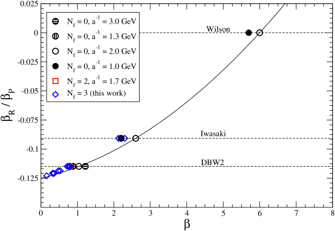
The RBC collaboration found that the combination of $\beta$ and $c_{1}$ that gives roughly the same lattice scale falls on the curve

$$\frac{\beta_{R}}{\beta_{P}}=-0.125+A(a)\beta+B(a){\beta}^{2},$$ (12)

where $\beta_{R}=c_{1}$ and $\beta_{P}=1-8c_{1}$. This is shown in Figure 1, where early simulations with $0$ and $2$ flavors of dynamical fermions and the simulations presented in this paper are included. The solid curve is a fit to the quenched simulations at an inverse lattice spacing of 2.0 GeV with different values of $\beta_{R}/\beta_{P}$. The ability to predict the lattice spacings in this manner allows us to do simulations at the desired coupling without the need for extensive searching in the parameter space.

While the QCDOC computers provide some of the most powerful resources currently available for lattice QCD, each parameter choice requires substantial computing resources. For example a 1,500 trajectory simulation takes a few weeks to generate on 1,024 nodes of QCDOC, depending on the quark masses and algorithms used. In our study, the choice of parameters often depended on ensembles running at that time, so it was important to generate ensembles as quickly as possible. We exploited naive parallelism and the availability of several smaller machines by spawning short Markov chains from the original chain. i.e. starting from a configuration in the original chain, a second distribution of random numbers (different from those in the original evolution) was generated and these were used to evolve a new branch. These branches were ‘farmed’ out to several machines in parallel. This had the advantage of increasing statistics to an acceptable level while reducing the ‘wall clock’ time.

We used the decomposition in Eq. (11) for the (D, 0.72, 0.01/0.04) and (D, 0.72, 0.04/0.04) ensembles, whereas for all the other ensembles, including the (D, 0.72, 0.02/0.04) ensemble, we combined the two 1/4 power determinants in the denominator of Eq. (11) into a single 1/2 power determinant and used one less pseudofermion field.

The parameters that enter into the RHMC algorithm control the accuracy of the rational approximation and the range of eigenvalues for which it is valid. Table 3 gives the value for the parameters we used. The maximum and minimum eigenvalues, $\lambda_{\rm max}$ and $\lambda_{\rm min}$, of ${\cal D}(m_{i})$ are used to determine the eigenvalue range for which the rational approximation has to be valid. The degree of the rational polynomial determines the accuracy of the approximation over this range. We use a more accurate rational approximation for the accept/reject step than for the molecular dynamics integration, since the accept/reject step removes any errors in the approximation arising during the integration.

Table 4 gives values for $\langle\delta H\rangle$, $\langle e^{-\delta H}\rangle$ and the acceptance for the ensembles generated with the RHMC algorithm. $\langle e^{-\delta H}\rangle$ is equal to $1$ within errors, indicating that the algorithm is working correctly. Also shown in Table 4 are the ensemble averages for the plaquette, where typically the first 1000 trajectories of the ensemble were excluded from the averages.

II.3 The static quark potential

The static quark potential depends relatively weakly on the sea quark masses. Consquequently, the chiral limit can be taken with reasonable confidence and provides an estimate of the lattice spacing that is relatively free of systematic uncertainty, compared to hadron masses.

The static potential $V(\vec{r})$ between a quark and anti-quark pair at relative spatial displacement $\vec{r}$ is calculated from the Wilson loop expectation value $\langle W(\vec{r},t)\rangle$, where

$$\langle W(\vec{r},t)\rangle=C(\vec{r})e^{-V(\vec{r})t}+{\rm excited}\ {\rm states}.$$ (13)

Here $\langle W(\vec{r},t)\rangle$ is the average of the standard Wilson loop with spatial side of length $\vec{r}$ and temporal extent $t$. The static quark potential is then given by the ratio

$$V(\vec{r},t)=\mathop{\rm ln}\Bigl{\{}\frac{W(\vec{r},t)}{W(\vec{r},t+1)}\Bigr{\}}.$$ (14)

The time dependence in $V(\vec{r},t)$ should disappear for sufficiently large $t$, so an important requirement is that $V(\vec{r})$ be determined from a plateau seen in the quantity $V(\vec{r},t)$ as $t$ increases for fixed $\vec{r}$.

We compute lattice values for the Wilson loops $\langle W(\vec{r},t)\rangle$ using the method of Bolder et al. Bolder:2000un . This approach evaluates all separations $\vec{r}$, including those which do not lie along a lattice axis. For such off-diagonal separations the Bresenham algorithm is used to determine the sequence of spatial gauge links that make up the spatial lines joining the two time segments of the Wilson loop. For both the on- and off-axis cases, these spatial links are constructed by APE smearing Albanese:1987ds to improve the ratio of signal to noise. To be precise, at each step of APE smearing we replace each spatial link by

$$U^{\prime}_{\mu}(x)\equiv\mathbb{P}\left[U_{\mu}(x)+c_{\rm smear,3d}\sum_{\nu=1,2,3\mu\not=\nu}\right. \left.\left(U_{\nu}(x)U_{\mu}(x+\hat{\nu})U^{\dagger}_{\nu}(x+\hat{\mu})+\right.\right.$$ (15)

$$\left.\!\!\!\!\!\!\!\!\!\!\!\!\!\!\!\!\!\!\!\!U^{\dagger}_{\nu}(x-\hat{\nu})U_{\mu}(x-\hat{\nu})U_{\nu}(x+\hat{\mu}-\hat{\nu})\right)\Bigg{]}\ \mu=\{1,2,3\},$$

where we include all spatial directions and $\mathbb{P}$ denotes a projection back onto $SU(3)$. This process is then repeated $N_{\rm smear,3d}$ times. The smearing coefficient and number of smearing steps are tuned to be $(c_{\rm smear,3d},N_{\rm smear,3d})=(0.50,20\sim 35)$, to maximise the overlap with the ground state of the Wilson loop, $C(\vec{r})$.

This approach was also used by the RBC collaboration Aoki:2004ht ; Hashimoto:2004rs and an earlier description of some of the results presented here can be found in Ref. Hashimoto:2005re . The results for $V(\vec{r})$ obtained by this procedure were checked by an independent calculation using only on-axis loops and Chroma code Edwards:2004sx . While the errors were much larger for times $t=5$ and 6, the results are consistent.

Physical parameters are obtained by fitting the lattice value of $V(\vec{r})$ to the function

$$V(\vec{r})=V_{0}-{\alpha\over|\vec{r}|}+\sigma|\vec{r}|.$$ (16)

Finally, the parameters $\alpha$ and $\sigma$ can be used to determine the Sommer scale Sommer:1993ce ; Guagnelli:1998ud

$$r_{0}(m_{l})=\sqrt{(1.65-\alpha)\over\sigma}$$ (17)

for each gauge action and gauge coupling $\beta$, in lattice units. The value of $r_{0}$ in the chiral limit can then be used to define the lattice spacing. To express this in physical units we take $a=0.5~{}{\rm fm}/r_{0}$.

II.4 Topological Charge

Continuum Yang-Mills gauge fields can be divided into classes characterized by an integer-valued winding number known as the Pontryagin index or topological charge:

$$Q=\frac{1}{32\pi^{2}}\int d^{4}x\;\epsilon_{\mu\nu\sigma\tau}\mathop{\rm tr}F_{\mu\nu}(x)F_{\sigma\tau}(x)\in\mathbb{Z}$$ (18)

which is stable under smooth deformations of the gauge field. The Atiyah-Singer index theorem Atiyah:1963_cd ; Atiyah:1968_cd predicts that the Dirac operator on a gauge background with topological charge $Q$ will have at least $Q$ exact zero modes in the zero quark-mass limit,

$$Q=n_{+}-n_{-},$$ (19)

where $n_{+}(n_{-}$) is the number of positive (negative) chirality zero modes.

On the lattice the situation is much more complicated; gauge fields are far from smooth and the low-energy form of the Dirac operator can be distorted by the explicit breaking of the continuum symmetries. Nonetheless, when using domain wall fermions, zero modes of the Dirac operator are apparent and their numbers have been found to correspond well with the value of the topological charge calculated from the gauge field (by methods described below)Blum:2000kn ; Blum:2001qg ; Aoki:2002vt . Given the numerical cost in solving for the low-lying eigenvalues of the domain wall Dirac operator, we apply two gluonic definitions of topological charge:

1. calculate the topological charge via Eq. (18) using a classically $O(a^{2})$-improved definition of the field strength tensor built from plaquette and rectangle clover-leaf terms (precise details can be found in Aoki:2004ht );

2. the ‘5Li’ definition of deForcrand:1995qq ; deForcrand:1997sq , which combines the $1\times 1$, $2\times 2$, $1\times 2$, $1\times 3$ and $3\times 3$ clover-leaf terms to give a classically $O(a^{4})$-improved definition of the field strength tensor and, therefore, of the topological charge using Eq. (18).

Since both these methods expand about the classical continuum limit, they cannot be directly applied to lattice gauge field configurations. Rather than deal with the subtle issue of constructing renormalised operators, we smooth the gauge field configurations so that expanding about the continuum limit is sensible. When using the first definition we follow DeGrand:1997ss in using APE smearing

$$U^{\prime}_{\mu}(x)\equiv\mathbb{P}\left[(1-c_{\mathrm{smear}})U_{\mu}(x)+\frac{c_{\mathrm{smear}}}{6}\sum_{\nu\not=\mu}\right. \left.\left(U_{\nu}(x)U_{\mu}(x+\hat{\nu})U^{\dagger}_{\nu}(x+\hat{\mu})+\right.\right.$$ (20)

$$\left.\left.U^{\dagger}_{\nu}(x-\hat{\nu})U_{\mu}(x-\hat{\nu})U_{\nu}(x+\hat{\mu}-\hat{\nu})\right)\right]\;,$$

with $c_{\mathrm{smear}}=0.45$ in which the temporal link is also smeared in contrast to Eq. (15). We quote the value of $Q$ after 20 steps, although we calculate up to 30 steps to check the stability of the extracted value. When using the second definition of topological charge, we follow deForcrand:1995qq ; deForcrand:1997sq and cool the configurations using the 5Li action. This takes the same combination of loops as used for the 5Li definition of the topological charge (although not clover-leaf symmetrized) to construct the action. Again, this definition is $O(a^{4})$-improved about the classical continuum limit. It is also chosen so that the size of the instantons is invariant under cooling for instantons of size a few lattice spacings. We have used up to 50 cooling steps. The results given in this paper are determined after 30 steps, beyond which the answers are stable.

A third method we have used to monitor the topological charge is to calculate the fermionic operator $\langle\bar{q}\gamma_{5}q\rangle$ using a stochastic estimator. We only used a single stochastic source per configuration and, therefore, this measurement has large fluctuations when $Q\not=0$, since the overlap of the noisy estimator with the small number of topological zero modes has a large variance. These fluctuations can be reduced by averaging measurements from nearby lattices in the Markov chain. At molecular dynamics time $\tau=i$, the smoothed value of $\langle\bar{q}\gamma_{5}q\rangle$ is found by averaging over measurements in the range $i-n/2\leq\tau<i+n/2$. We refer to this as a smoothing window of size $n$. Smoothing suppresses topological fluctuations that exist for only a short time in the evolution and should give a good estimator of the topological charge if the topology only changes significantly on a molecular dynamics timescale that is larger than $n$. The three methods give measurements of $Q$ that agree extremely well.

II.5 Hadron masses

Hadronic correlation functions are constructed from quark propagators which take the following form

$$S_{AB}(x,y)=\langle q_{A}(x)\overline{q}_{B}(y)\rangle,$$ (21)

where the indices $A$ and $B$ represent different smearings of the quark field, $q(x)$. All the smeared quark fields make use of the same construction of the four-dimensional quark field from the five-dimensional domain wall fermion field $\Psi(x,s)$. In the case of the local ($L$) quark field, $q_{L}(x)$, this takes the form

$$q_{L}(x)=P_{L}\Psi(x,s=0)+P_{R}\Psi(x,s=(L_{s}-1))\,$$ (22)

where $P_{R/L}=\frac{1}{2}\left(1\pm\gamma_{5}\right)$ are the chiral projectors. To construct the Coulomb gauge-fixed wall sources ($W$), we replace the quark field in Eq. (21) with the non-local field

$$q_{W}(t)_{c}=\sum_{r,c^{\prime}}V\left(r,t\right)_{c,c^{\prime}}q_{L}(r,t)_{c^{\prime}}$$ (23)

where $V(r,t)$ is the color matrix which transforms the spatial links at $x=(r,t)$ into Coulomb gauge and $c$ and $c^{\prime}$ are color indices. The third type of smearing ($S$) uses a hydrogenic wavefunction Boyle:1999gx . The quark field is convolved with a spatial smearing function after fixing the gauge fields to the Coulomb gauge as follows,

$$q_{S}(t)_{c} = \sum_{r,r^{\prime},c^{\prime}}S\left(r,r^{\prime}\right)V\left(r^{\prime},t\right)_{c,c^{\prime}}q_{L}(r^{\prime},t)_{c^{\prime}}\,,$$ (25)

$$S(r,r^{\prime})=e^{(-\Delta r/R)}\delta_{r,r_{0}}\,,$$

where $\Delta r$ is the modulus of the minimum distance between the center of the source, $r_{0}$, and $r^{\prime}$ (taking into account the periodic boundary conditions), and $R$ is a tunable parameter. We give detailed comparisons of results for hadron masses obtained with different smearings in Section III.

Correlation functions for mesonic operators are constructed as follows

$$C_{ij}(t,\vec{p})=\sum_{\vec{x}}e^{i\vec{p}\cdot\vec{x}}\langle\Omega_{i}(\vec{x},t)\Omega^{{\dagger}}_{j}(\vec{0},0)\rangle$$ (26)

where

$$\Omega_{i}(\vec{x},t)=q(\vec{x},t)\Gamma_{i}\bar{q}(\vec{x},t)$$ (27)

and, for instance, $\Gamma_{i}=\gamma_{5}$ for the pseudoscalar meson and $\Gamma_{i}=\gamma_{k}$ for the vector meson. The spectrum can then be extracted by fitting these correlation functions at zero momentum to the form

$$C(t)=\sum_{n}A_{n}\left(e^{-m_{n}t}+e^{-m_{n}(T-t)}\right)$$ (28)

where $T$ is the size of the lattice in the time direction. For sufficiently large $t$, the ground state will dominate the correlation function.

The standard baryon interpolating operator is composed of a local diquark operator and a spectator-like quark field:

$$\Omega_{ijk,B}(x)=\epsilon_{abc}\left[q^{T}_{a,i}(x)C\Gamma q_{b,j}(x)\right]q_{c,k}(x),$$ (29)

where $\Gamma$ stands for one of the possible 16 Dirac matrices and $C$ is the charge conjugation matrix. The superscript $T$ denotes transpose and the indices $abc$ and $ijk$ label color and flavor, respectively. For the $(I,J)=(\frac{1}{2},\frac{1}{2})$ baryons (the nucleon), an iso-scalar diquark is chosen, i.e $\{\Gamma=1,\gamma_{5},\gamma_{5}\gamma_{\mu}\}$. However, only two of the three operators are independent, as they are related to each other through a Fierz transformation. In this work, the two nucleon operators are chosen to be

$$\Omega_{B_{1}} = \epsilon_{abc}\left[u^{T}_{a}C\gamma_{5}d_{b}\right]u_{c},$$ (30)

$$\Omega_{B_{2}} = \epsilon_{abc}\left[u^{T}_{a}Cd_{b}\right]u_{c}.$$ (31)

The intrinsic parity of these operators is defined by the parity transformation of the internal quark fields. The $\Omega_{B_{1}}$ ($\Omega_{B_{2}}$) operator transforms as a positive (negative) parity operator. However, this parity assignment is easily flipped by multiplication of the local baryon interpolating operator by $\gamma_{5}$. Therefore, a two-point correlation function composed of either $\Omega_{B_{1}}$ or $\Omega_{B_{2}}$ operators possesses both the positive- and negative-parity nucleon contributions. For details, see Ref. Sasaki:2001nf ; Sasaki:2005ug . The $\Omega_{B_{1}}$ operator is conventionally used in lattice QCD for the $J^{P}=1/2^{+}$ nucleon ($N$). However, it is also of interest to examine the $J^{P}=1/2^{-}$ nucleon ($N^{*}$), so both $\Omega_{B_{1}}$ and $\Omega_{B_{2}}$ operators are utilized for $(I,J)=(\frac{1}{2},\frac{1}{2})$ baryon spectroscopy.

Taking the trace of the baryon two-point correlator with the relevant projection operator, $P_{+}=(1+\gamma_{4})/2$, the two-point correlator in a finite box with (anti-) periodic boundary conditions is given by

$$C_{B}(t)=A_{\eta}e^{-m_{\eta}t}-A_{-\eta}e^{-m_{-\eta}(T-t)},$$ (32)

where the parity of the forward propagating state $\eta=+$ ($-$) is the same as the intrinsic parity of the interpolating operator, $\Omega_{B_{1}}$ ($\Omega_{B_{2}}$), whilst the backward propagating state has the opposite parity.

According to an intensive study of the nucleon excited states in Ref. Sasaki:2001nf , the $\Omega_{B_{2}}$ operator has a poor overlap with the nucleon ground state. Therefore, in this study, the masses of the positive and negative parity states were determined by a simultaneous fit to the following forms

$$C_{B_{1}}(t) = A_{+}e^{-m_{+}t}-A_{-}e^{-m_{-}(T-t)},$$ (33)

$$C_{B_{2}}(t) = A^{\;{}^{\prime}}_{-}e^{-m_{-}t}.$$

II.6 Residual mass

While at short distances the domain wall fermion formulation is a five-dimensional lattice theory, at long distances and for large $L_{s}$ it is expected to appear identical to continuum QCD, with chiral symmetry broken only by the explicit mass term $m_{f}$, introduced in Eq. (6). The deviations from this ideal behaviour can be easily described by a continuum, Symanzik effective Lagrangian. Because of the finite size of the fifth dimension, this effective Lagrangian will contain explicit chiral symmetry breaking terms. While the coefficients of these terms are suppressed as $L_{s}$ increases, they are important because of their chiral properties and because they are of lower dimension (three and five) than the dimension-six, chirality conserving, $O(a^{2})$ terms:

$${\cal L}_{\rm eff}=L_{\rm QCD}(m_{f}=0)+(m_{f}+m_{\mbox{\tiny res}})\overline{q}q+c_{5}\overline{q}\sigma^{\mu\nu}F^{\mu\nu}q.$$ (34)

The leading term is simply an additional mass term whose coefficient is called the residual mass, labelled $m_{\mbox{\tiny res}}$. As is conventional, the normalization of $m_{\mbox{\tiny res}}$ is fixed by requiring the input parameter $m_{f}$ and $m_{\mbox{\tiny res}}$ to multiply the same $\overline{q}q$ mass operator as in Eq. (34). In this paper we will ignore the effects of the Sheikholeslami-Wohlert, $c_{5}$ term, which is suppressed by both large $L_{s}$ and one power of the lattice spacing. As will be seen below, methods for determining $m_{\mbox{\tiny res}}$ typically determine a quantity which depends on the input quark mass $m_{f}$. This $m_{f}$ dependence is a lattice artefact and represents the $O(a)$ or $O(a^{2})$ ambiguity in our definition of $m_{\mbox{\tiny res}}$. A more careful treatment, which requires the analysis of the $c_{5}$ term in Eq. (34) and similar lattice artefacts in the quantities being used to compute $m_{\mbox{\tiny res}}$ is beyond the scope of this paper.

The residual mass can be computed from the additional contribution to the partially conserved axial current, $J^{a}_{5q}$, at the mid-point of the fifth dimension Furman:1994ky ; Blum:1998ud ; Blum:2000kn . Assuming that this mid-point contribution can also be described using the Symanzik effective theory of Eq. (34), then to lowest order in the quark mass and lattice spacing $J^{a}_{5q}=m_{\mbox{\tiny res}}J^{a}_{5}=m_{\mbox{\tiny res}}\overline{q}\gamma^{5}t^{a}q$, where $t^{a}$ is a generator of the flavor symmetry. We can then compute $m_{\mbox{\tiny res}}$ by averaging over time the quantity $R(t)$, which is defined by

$$R(t)=\frac{\langle\sum_{\vec{x}}J^{a}_{5q}(\vec{x},t)\pi^{a}(0)\rangle}{\langle\sum_{\vec{x}}J^{a}_{5}(\vec{x},t)\pi^{a}(0)\rangle}.$$ (35)

Here $\pi^{a}(0)$ is a (possibly smeared) pseudoscalar interpolating field at $t=0$. The minimum time used in the average need only be large enough to remove any contribution to the correlators in $R(t)$ from unphysical states, since $m_{\mbox{\tiny res}}$ should affect all physical states equally. In the following we will refer to this average of $R(t)$ as $m_{\mbox{\tiny res}}^{\prime}(m_{f})$ to explicitly display its dependence on $m_{f}$ and to allow a clear discussion of how we deal with this small, non-zero lattice spacing ambiguity in determining the constant $m_{\mbox{\tiny res}}$ which appears in the effective Lagrangian of Eq. (34).

II.7 Determining the pseudoscalar decay constant

The pseudoscalar decay constant is defined by

$$Z_{A}\langle 0|\,\bar{q}(x)\gamma^{\mu}\gamma_{5}q(x)\,|\pi,\vec{p}\rangle=-if_{P}p^{\mu}e^{-ip\cdot x}$$ (36)

where $Z_{A}$, the renormalization factor for the local axial vector current, can easily be determined for domain wall fermions since $Z_{A}A^{a}_{\mu}={\cal A}^{a}_{\mu}$ and ${\cal A}^{a}_{\mu}$ is the (partially) conserved axial current. In particular, we follow Blum:2000kn and define

$$C(t+1/2) = \sum_{\vec{x}}\langle{\cal A}^{a}_{0}(\vec{x},t)\;\pi^{a}(\vec{0},0)\rangle$$

$$L(t) = \sum_{\vec{x}}\langle A^{a}_{0}(\vec{x},t)\;\pi^{a}(\vec{0},0)\rangle.$$ (37)

We then calculate $Z_{A}$ from these correlators, using a combination that is free of ${\cal O}(a)$ errors and minimizes ${\cal O}(a^{2})$ errors. This gives us the following explicit form for $Z_{A}$.

$$Z_{A}=\frac{1}{1+t_{\rm max}-t_{\rm min}}\sum_{t=t_{\rm min}}^{t_{\rm max}}\frac{1}{2}\left\{\frac{C(t+1/2)+C(t-1/2)}{2\ L(t)}+\frac{2\ C(t+1/2)}{L(t)+L(t+1)}\right\}.$$ (38)

We have calculated $f_{P}$ in three ways. The simplest uses the local-local axial current in Eq. (26), giving

$$C^{LL}_{A_{0},A_{0}}(t)=\sum_{\vec{x}}\langle 0|A_{0}(\vec{x},t)\;A_{0}(0,0)|0\rangle\to A^{LL}_{A_{0},A_{0}}(e^{-mt}+e^{-m(T-t)}).$$ (39)

The amplitude $A^{LL}_{A_{0},A_{0}}$ is determined from fitting the correlator to Eq. (39), which in turn using Eq. (36) yields $f_{P}$ from

$$f_{P}=Z_{A}\sqrt{\frac{2A^{LL}_{A_{0},A_{0}}}{m_{P}}}.$$ (40)

In the second method, we use the axial Ward-Takahashi identity which, including the midpoint contribution as $J^{a}_{5q}=m_{\mbox{\tiny res}}J^{a}_{5}$, gives

$$m_{P}Z_{A}\langle 0|A_{0}|\pi\rangle=2(m_{f}+m_{\mbox{\tiny res}})\langle 0|P|\pi\rangle$$ (41)

where $P$ is the pseudoscalar density. From the local-local pseudoscalar correlator, we have

$$C^{LL}_{P,P}(t)=\sum_{\vec{x}}\langle 0|P(\vec{x},t)\;P(0,0)|0\rangle\to A^{LL}_{P,P}(e^{-m_{P}t}+e^{-m_{P}(T-t)})$$ (42)

which, combined with Eq. (36), gives

$$f_{P}=\frac{2(m_{f}+m_{\mbox{\tiny res}})}{m_{P}}\;\sqrt{\frac{2A^{LL}_{P,P}}{m_{P}}}.$$ (43)

The third method uses the local axial current pseudoscalar correlator

$$C^{LL}_{A_{0},P}(t)=\sum_{\vec{x}}\langle 0|A_{0}(\vec{x},t)\;P(\vec{0},0)|0\rangle\to\frac{\langle 0|A_{0}|\pi\rangle\langle\pi|P|0\rangle}{2m_{P}}(e^{-m_{P}t}+e^{-m_{P}(T-t)}).$$ (44)

The ratio of this correlator and the pseudoscalar density correlator is then fitted to the following form,

$$\frac{C_{A,P}(t)}{C_{P,P}(t)}=\frac{\langle 0|A_{0}|\pi\rangle\langle\pi|P|0\rangle}{\langle 0|P|\pi\rangle\langle\pi|P|0\rangle}\approx\frac{\langle 0|A_{0}|\pi\rangle}{\langle 0|P|\pi\rangle}\tanh\left[m_{P}(\frac{T}{2}-t)\right],$$ (45)

to yield

$$A_{A_{0},P}=\frac{\langle 0|A_{0}|\pi\rangle}{\langle 0|P|\pi\rangle}.$$ (46)

Using the amplitude from the fit to the pseudoscalar density correlator, together with the value of $Z_{A}$, we obtain an expression for the pseudoscalar decay constant as

$$f_{P}=Z_{A}\sqrt{\frac{2A_{P,P}}{m_{P}}}A_{A_{0},P}.$$ (47)

Comparing these different extractions allows us to probe the systematic error due to both mass and amplitude extraction, and the degree to which the chiral Ward identity is satisfied after shifting $m_{f}\rightarrow m_{f}+m_{\rm res}$.

II.8 Autocorrelation length

The integrated autocorrelation time is defined as Allton:1998gi ; Autocorr

$$\tau^{{\rm int}}_{A}=\frac{1}{2}\sum^{\infty}_{-\infty}\rho_{A}(t)=\frac{1}{2}+\sum^{\infty}_{t=1}\rho_{A}(t)$$ (48)

where the autocovariance function, $\rho_{A}(t)$ defines the exponential autocorrelation time $t_{exp}$

$$\rho_{A}(t)=\frac{\Gamma_{A}(t)}{\Gamma_{A}(0)},\quad\rho_{A}(t)\stackrel{{\scriptstyle t\rightarrow\infty}}{{\rightarrow}}e^{-t/\tau_{{\rm exp}}}$$ (49)

and the autocovariance of an observable $A$ is

$$\Gamma_{A}(t)=\langle(A_{s}-\langle A\rangle)(A_{s+t}-\langle A\rangle)\rangle.$$ (50)

The subscripts $t$ and $s$ label the Monte Carlo time and the outer average is over all pairs separated by $t$. It is standard to consider configurations separated by $2\tau_{A}^{{\rm int}}$ to be statistically independent.

In practice, we truncate the sum in Eq. (48) at some finite value, $t_{{\rm max}}$, and define the cumulative autocorrelation time to be

$$\tau_{A}^{{\rm cum}}=\frac{1}{2}+\sum_{t=1}^{t_{\rm max}}\rho_{A}(t).$$ (51)

In the limit of sufficiently large $t_{\rm max}$, this will be a good approximation to $\tau_{A}^{\rm int}$. In order to obtain reliable estimates for $\tau_{{\rm exp}}$ and $\tau^{{\rm cum}}_{A}$, autocorrelations should ideally be measured using ensembles containing many more configurations than the value of $\tau^{{\rm int}}_{A}$. Conversely, it must be noted that the measurement of the autocorrelation time is not sensitive to correlations over ranges of trajectories that are an appreciable fraction of the ensemble length, or greater.

III Results

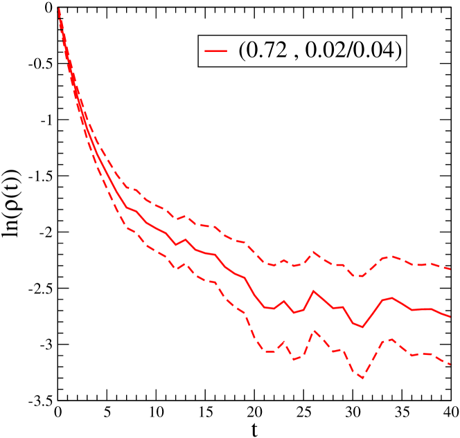
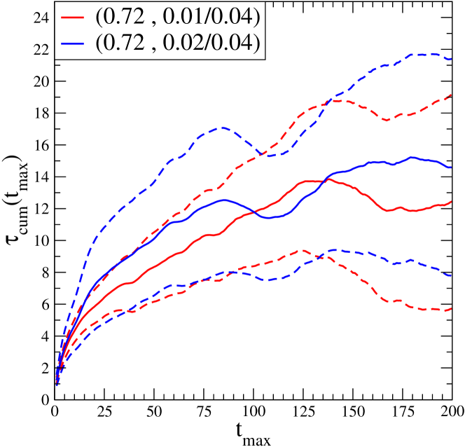
Figures 2 and 3 shows example plots for the autocorrelation function and the integrated autocorrelation length for the plaquette and the pseudoscalar meson correlator at timeslice 12. The statistical errors plotted for $\rho_{A}(t)$ and $\tau_{{\rm cum}}$ were estimated using a jackknife procedure. In order to take into account the effects of autocorrelations in the error estimates for $\rho(t)$ and $\tau_{{\rm cum}}$ themselves, the original data for $\rho(t)$ and $\tau_{{\rm cum}}$ were grouped in bins of size $b$. Bin size was increased until the size of the jackknife errors stabilised to give the error bands shown on the plots. The final results can be found in Table 5, for both the DBW2 $\beta=0.72$ and Iwasaki $\beta=2.13$ RHMC datasets (the other ensembles are much shorter, and so the results are not given).

III.1 Static quark potential

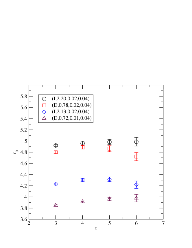
The results for the values of the parameters $V_{0}$, $\alpha$, $\sigma$ and $r_{0}$ in Eq. (16) and (17) are given in Table 6. These are obtained by using the fitting range $r\in[\sqrt{3},8]$ and the choice $t=5$ in Eq. (14). The first error in $r_{0}$ given in the table is statistical and the second is an estimate of the systematic error in the fitting procedure. This estimate of systematic error is determined from the shift in the central value when the limits of the fitting range in $r$ are swept through $r_{\rm min}\in[\sqrt{2},\sqrt{6}]$ and $r_{\rm max}\in[7,9]$ and $t$ is changed from 5 to 6. In Figure 4 we show some example plateaux found for $r_{0}$ as $t$ is varied between 3 and 6, suggesting a reasonably stable result and good suppression of excited states by $t=5$.

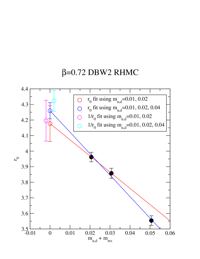
In Table 7 we list the result for $r_{0}$ that we obtain from a simple linear extrapolation to vanishing light sea quark mass for the four ensembles where we have two or more values for the light sea quark mass. Figure 5 compares two extrapolations for the DBW2 $\beta=0.72$ ensembles where we use either the two lightest mass values, $m_{l}=0.01$ and 0.02 or all three $m_{l}=0.01$, 0.02, and 0.04.

III.2 Topological Charge

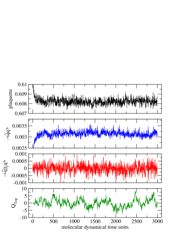
The time histories of the plaquette $\langle\bar{q}q\rangle$, $\langle\bar{q}\gamma_{5}q\rangle$ and the topological charge, are plotted in Figure 6 for the (D, 0.72, 0.01/0.04) ensemble. Measured values are plotted every 10 trajectories (5 molecular dynamics time units). This ensemble has the smallest values for $m_{l}$, and these time histories make our choice of 500 time units for thermalization appear reasonable.

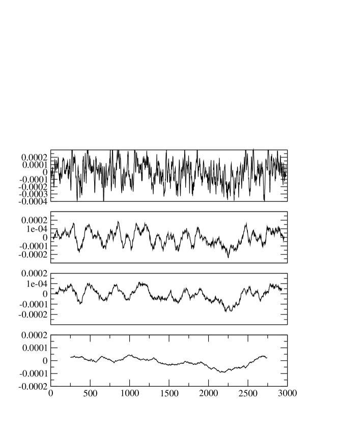
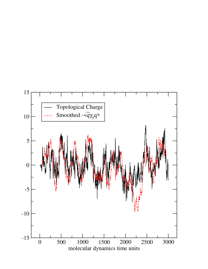
The topological charge in the bottom panel of Figure 6 was measured using gluonic method 1, as described in Section II.4. We can compare this with a fermion based definition of topology using $\langle\bar{q}\gamma_{5}q\rangle$. To make this comparison, Figure 7 gives the evolution of a smoothed version of $\langle\bar{q}\gamma_{5}q\rangle$ for the (D, 0.72, 0.01/0.04) ensemble, with smoothing windows of size 25, 50, 100 and 200 time units. Comparing these evolutions with the unsmoothed $\langle\bar{q}\gamma_{5}q\rangle$ evolution in the third panel of Figure 6 reveals noise is substantially reduced by smoothing. The relevance of the resulting signal can be seen by comparing with the evolution of the topology as measured from the gauge field. Figure 8 directly compares this estimate of the evolution of topological charge with the evolution of $\langle\bar{q}\gamma_{5}q\rangle$, which has been smoothed with a window size of 50. The data are strongly correlated and show good agreement between topology as determined from smeared gauge links and from the Dirac operator. Since smoothing the data changes its normalization, we have rescaled the smoothed data such that its largest value is equal to that of the largest value of topological charge from the gauge field.

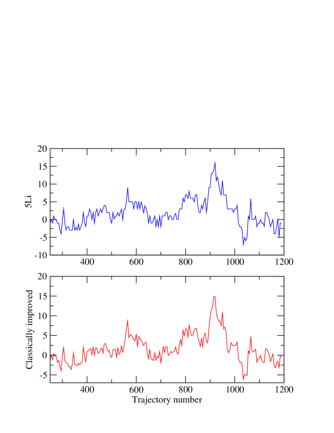
A comparison of 5Li and classically improved methods has been performed on the (I, 2.13, 0.04/0.04) ensemble. Figure 9 shows the topological charge history from the two methods As can be seen they track each other quite well, although they disagree in places by as much as $\sim 3$ units of topological charge. It can also be noted that the 5Li method give results which are much better aligned with integers than the classically improved method.

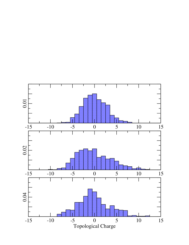
As a whole, while the topological charge is certainly not completely decorrelated from configuration to configuration, this set of ensembles are sampling the topological sectors quite well. This can also be seen in the histograms shown in Figure 10.

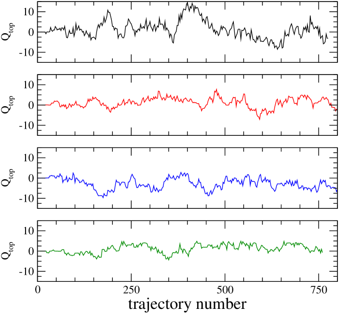
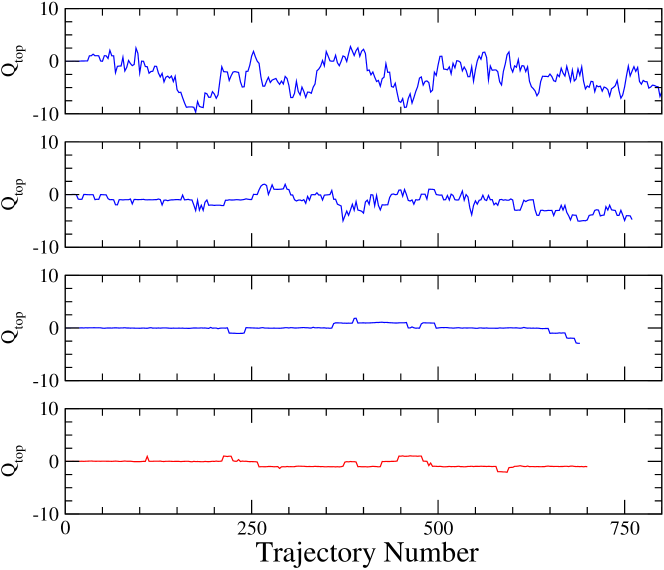
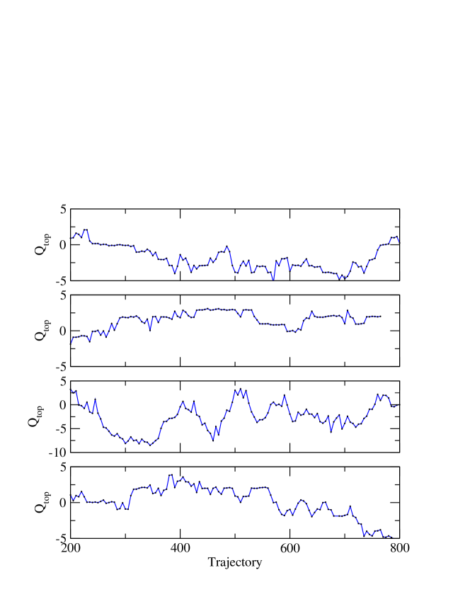
Figure 11 shows the gluonic measure of the topological charge for the large rectangle simulations at fixed lattice spacing. Although the topological charge is sampled well between $-15$ and 15 for the (D, 0.72, 0.04/0.04, R) ensemble (top panel), as we make $c_{1}$ more negative, the range of the topological charge we are able to sample tends to narrow. For the (C7.47, 0.16, 0.04/0.04, R) ensemble (bottom panel), the topological charge fluctuates only in the range of $\pm 5$, and it takes a large number of trajectories to move between different topology sectors. The situation is worse at weaker couplings, where the topological charge evolution is much slower. This can be seen in Figure 12, where the top three panels have a rectangle coefficient of $c_{1}=-3.57$ and the bottom one has $c_{1}=-2.3$. In the absence of a dramatic improvement in the chiral properties of domain wall fermions, this is a compelling reason to avoid larger rectangle coefficients. As should be expected, these trends with rectangle coefficient and coupling also apply to the DBW2 and Iwasaki actions. Figure 13 shows – from top to bottom – representative topological charge histories for the DBW2 action with $\beta=0.764$ and $\beta=0.78$, and the Iwasaki action with $\beta=2.13$ and $\beta=2.2$.

III.3 Hadron masses

Hadronic correlation functions were constructed from quark propagators which were smeared at the source and local at the sink, as described in Section II.5. We use the following notation to describe the combinations of smearing: ${\rm S}_{1}{\rm F}_{1}-{\rm S}_{2}{\rm F}_{2}$, where ${\rm S}_{i}$ denotes source and ${\rm F}_{i}$ sink for the quark propagators $i=\{1,2\}$ in the meson correlator. In particular, four combinations were computed: LL-LL, SL-LL, SL-SL, and WL-WL. The first combination has the attractive property that, as both meson interpolating operators are the same, the ground state and all the excited state contributions to the correlation function are positive. The effective mass,

$$M^{\rm eff}(t)=\log{\left[\frac{C(t)}{C(t+1)}\right]},$$ (52)

which is used to determine when the ground state is dominating the correlation function, then approaches a plateau from above and can be used to determine unambiguously a fitting range for a single exponential function. Smeared and wall sources have the advantage that the plateau, and hence the fitting range that can be used, starts earlier.

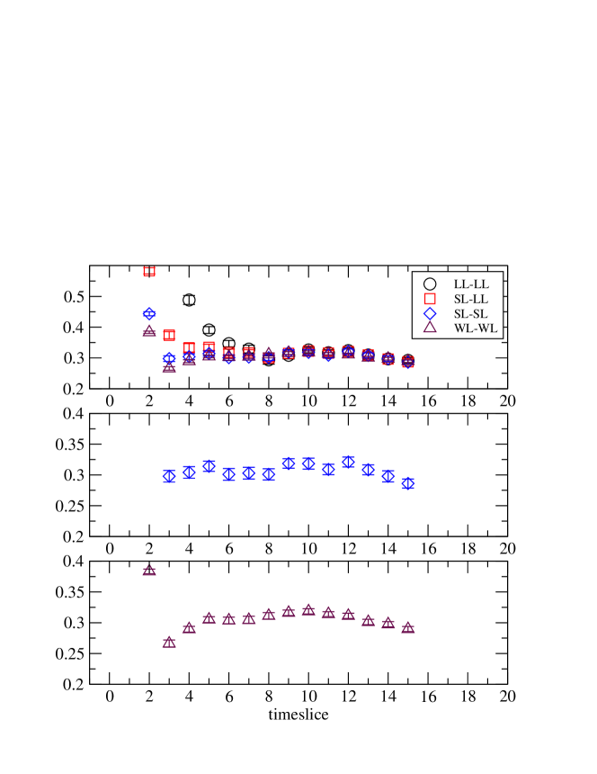
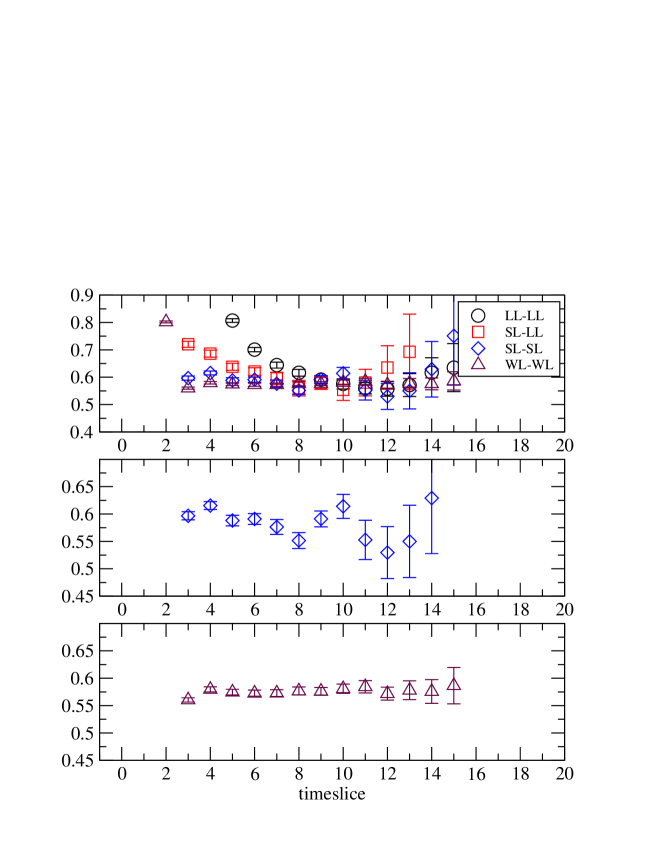
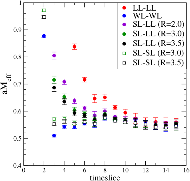
Figure 14 shows the pseudoscalar effective mass for four different source/sink combinations as determined from the pseudoscalar-pseudoscalar correlator for the (D, 0.72, 0.01/0.04) ensemble, while Figure 15 shows a similar plot for the vector meson effective mass. In both cases, the mesons are constructed from degenerate mass quarks with $m_{\rm val}=0.01$. These plots use a radius of 3.0 for the smearing function ($R$ in Eq.( 25)), which was found to be approximately optimal for both the pseudoscalar meson and the vector meson. This can be seen from Figure 16, which shows a comparison of the vector meson effective mass for various different smearing radii on the (I, 2.2, 0.02/0.04) ensemble with a valence quark mass of 0.04. When multiple sources are available, we have also extracted the mass by simultaneously fitting a pair of correlators with different sources to the ground and first excited state. The advantage of this approach is that the systematic uncertainty in the ground state mass arising from the choice of fit range is reduced. In summary, with careful choices of fitting ranges all the sources used in this work give consistent results.

The extracted pseudoscalar meson masses for the cases where valence and sea quark masses are equal, i.e. unitary data, are given in Table 8 for all of the RHMC ensembles. For the DBW2 gauge action at $\beta=0.72$ we also have data for which the valence quarks are not degenerate with the sea quarks. These results are given in Table 9. The corresponding results for the vector meson masses are given in Tables 10 and 11 respectively.

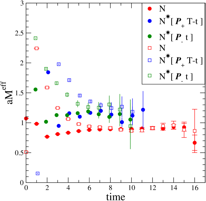
As with the construction of the meson operators, smeared quark fields are used to construct improved nucleon interpolating fields. In particular, all the data presented were extracted using correlators in which one interpolating operator is constructed from local quark fields, while the other interpolating operator is either constructed from smeared quark fields (denoted SL-SL-SL), or gauge-fixed wall sources (denoted WL-WL-WL). Figure 17 shows a typical effective mass plot for the nucleon. The backwards propagating, negative parity state in the standard nucleon correlator has been reflected about the middle of the time axis. Both states are shown together in Figure 17, where solid symbols represent data obtained from the WL-WL-WL correlators while open symbols correspond to the SL-SL-SL correlators. Fits to either type of smearing produce the same nucleon mass within the measured uncertainties.

The mass of the negative-parity nucleon is less well determined due to the poor signal and has some dependence on the type of smearing chosen. Moreover, the physical volume of these lattices is likely to be too small to extract accurately orbitally excited baryon states such as the $N^{\star}$. However, the data presented can be used in combination with larger volume runs to estimate the size of the finite volume effects on the remaining spectrum. The extracted values of the nucleon mass are collected in Table 12. The three fit ranges given are for the forwards propagating state $(N_{+})$, the backwards propagating state $(N_{-})$, and the negative parity correlator $(N^{\prime}_{-})$.

III.4 The residual mass

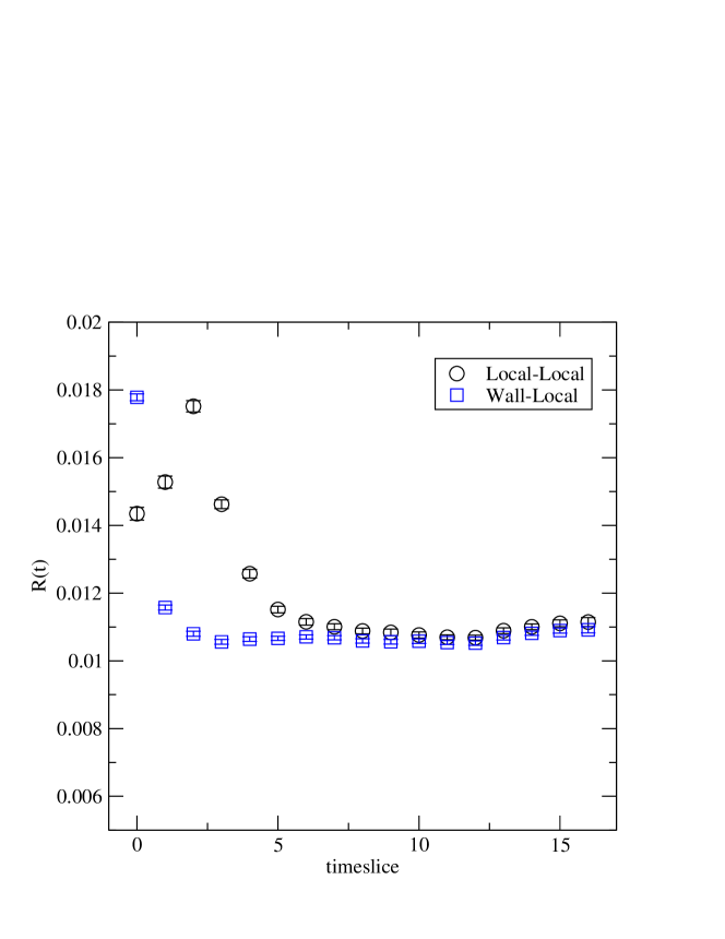
The ratio $R(t)$ given in Eq. (35) is shown in Figure 18 for the ensemble (D, 0.72 0.01/0.04). Since the correlator is time symmetric, the data shown is the average of the two halves of the lattice. This ratio should be constant as long as the separation in time is large enough that the effects of non-physical states/non-locality are eliminated. For the LL-LL correlator this is from $t\geq 7$ in the figure, but it is earlier for the WL-WL correlator as the overlap of the smeared operator with the physical states is larger in this case. As discussed above in Section II.6, we refer to this average of $R(t)$ as $m_{\mbox{\tiny res}}^{\prime}(m_{f})$, to distinguish it from the constant $m_{\mbox{\tiny res}}$ which appears in the Lagrangian of Eq. (34). The values of $m_{\mbox{\tiny res}}^{\prime}(m_{f})$ from the unitary data are given in Table 13 and from the non-degenerate data in Table 14.

Table 15 contains the results for $m_{\mbox{\tiny res}}^{\prime}(m_{f})$ and the vector meson mass as the magnitude of the rectangle coefficient $c_{1}$ is increased. In this case $m_{\mbox{\tiny res}}^{\prime}(m_{f})$ has been estimated by averaging $R(t)$ from $t=4$ to $t=16$. The decrease in $m_{\mbox{\tiny res}}$ as $|c_{1}|$ increases is expected, since the non-locality introduced by the large rectangle term suppresses the fluctuations of the gauge fields on the scale of two lattice spacings, and the number of low-lying localized modes is moderately reduced Antonio:2005wm . If a small residual mass were the only consideration for our parameter choices, our goal could be accomplished by increasing the magnitude of the rectangle coefficient. However, we would forfeit our ability to tunnel between different topological sectors, as shown in the previous section. It is for this reason that we concentrated on the Iwasaki and DBW2 actions in our more extensive action studies.

III.5 $Z_{A}$ and the pseudoscalar decay constant

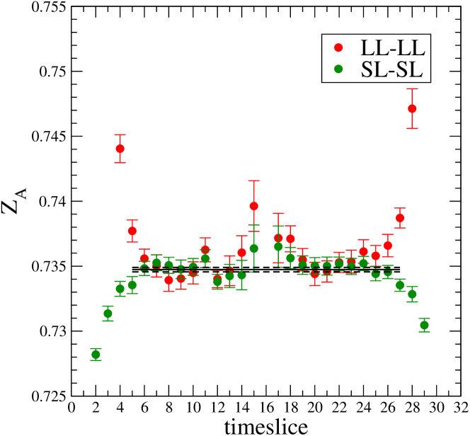
The value of $Z_{A}$ is determined from Eq. (38), using either LL-LL or SL-SL correlators. In the case when smearing is used, this corresponds to using a smeared-smeared pseudoscalar interpolating field in Eq. (37). Since the axial current operator is unchanged, this still corresponds to an extraction of the renormalization factor for the local axial current, $A_{\mu}^{a}$. Figure 19 shows a comparison of two such extractions for the (D, 0.72, 0.02/0.04) ensemble, with good agreement being found. The values of $Z_{A}$ for the unitary data are given in Table 16. For the (D, 0.72, 0.01/0.04) ensemble we also have some partially quenched data, extracted using LL-LL correlators. The values are given in Table 17.

The value of the pseudoscalar decay constant has been determined in three ways according to Eq. (40), (43) and (47). These results are presented for both the unitary and non-unitary data in Tables 18-21. Figure 20 shows an example of the third method (Eq. (47)) for the DBW2 $\beta=0.72$ ensembles.

III.6 Chiral extrapolations and results for phenomenological quantities

To estimate values of phenomenologically relevant quantities requires extrapolating our data to the physical $u$ and $d$ quark masses. For the DBW2 $\beta=0.72$ ensembles we have three sea-quark mass values, as well as non-degenerate valence quark masses, enabling us to explore the extent to which our data agrees with the predictions of leading order (LO) or next-to-leading order (NLO) (partially quenched) chiral perturbation theory (PQ$\chi$PT). Preliminary work on this data can be found in Lin:2005gh . For the remaining DBW2 and Iwasaki ensembles, we only have two sea-quark mass values and so only linear extrapolations are possible. For the larger rectangle ensembles, only one sea-quark mass was generated, so valence only extrapolations are performed.

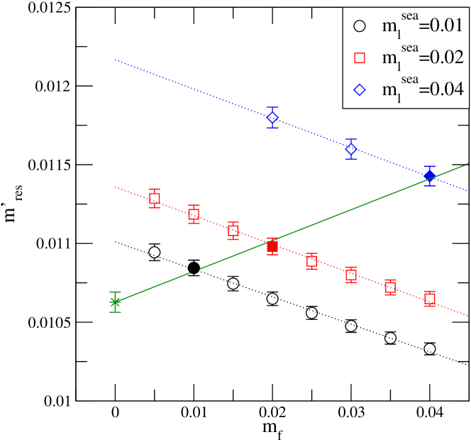
For each of these extrapolations we must include the effects of the residual quark mass which should be treated as an addition to the explicit quark mass $m_{f}$. Thus, the chiral limit should be defined as that value of $m_{f}$ for which $m_{f}+m_{\mbox{\tiny res}}=0$. Our values for the residual mass, $m_{\mbox{\tiny res}}^{\prime}(m_{f})$, determined from the midpoint term in the axial current divergence, themselves depend on $m_{f}$, a lattice artefact. We treat this $m_{f}$ dependence in two different ways where we have three sea-quark masses. Firstly we extrapolate linearly in $m_{f}$ to define $m_{\mbox{\tiny res}}=m_{\mbox{\tiny res}}^{\prime}(m_{f}=0)$ for the unitary data, giving $m_{\mbox{\tiny res}}=0.0106(1)$. This is shown in Figure 21. Secondly we construct the quark mass

$$m_{q}=m_{f}+m_{\mbox{\tiny res}}^{\prime}(m_{f})$$ (53)

and extrapolate hadronic quantities versus $m_{q}$ to $m_{q}=0$. For data where we have two sea-quark masses we follow the second procedure. These two procedures adopt slightly different choices for the residual mass: $m_{\mbox{\tiny res}}=m_{\mbox{\tiny res}}^{\prime}(m_{f}=0)$ and $m_{\mbox{\tiny res}}=m_{\mbox{\tiny res}}^{\prime}(m_{f}=-m_{\mbox{\tiny res}})$. The difference between these two approaches is at most a few percent and reflects a non-zero lattice spacing error that we do not attempt to control in this paper.

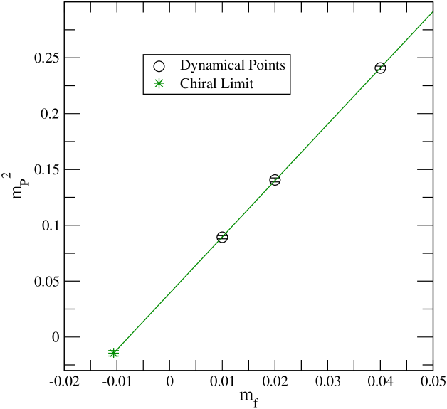
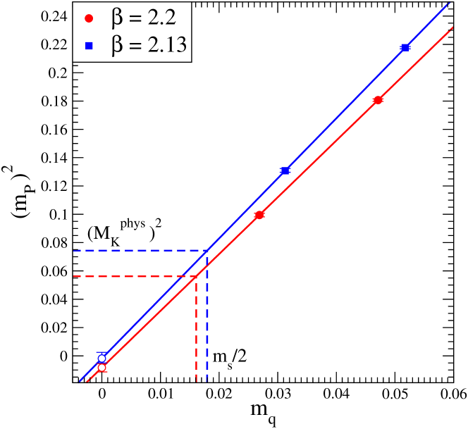
Concentrating on the DBW2 $\beta=0.72$ ensembles, Figure 22 plots the square of the pseudoscalar meson mass from the unitary data versus $m_{f}$. Lowest order chiral perturbation theory would suggest that this should be linear in the mass, and extrapolate to zero in the $m_{f}=-m_{\rm res}$ limit. This is not exactly obeyed, $m_{P}^{2}$ extrapolates to $-0.0144(24)$ at $m_{f}=-m_{\rm res}$. This is due to the relatively small size of the fifth dimension. Conversely, vanishing pseudoscalar meson mass occurs at a value of $m_{f}=-0.0078(5)$. Whilst this represents a relatively large discrepancy with the definitions of zero quark mass used above, and is much bigger than the discrepancy in the definitions of $m_{\mbox{\tiny res}}$, it is itself a small effect when compared to the statistical uncertainties of other hadron masses and matrix elements extrapolated to the chiral limit. Ultimately, the uncertainty in the value of $m_{\mbox{\tiny res}}$ is not the dominant source of uncertainty in the value of any results presented here.

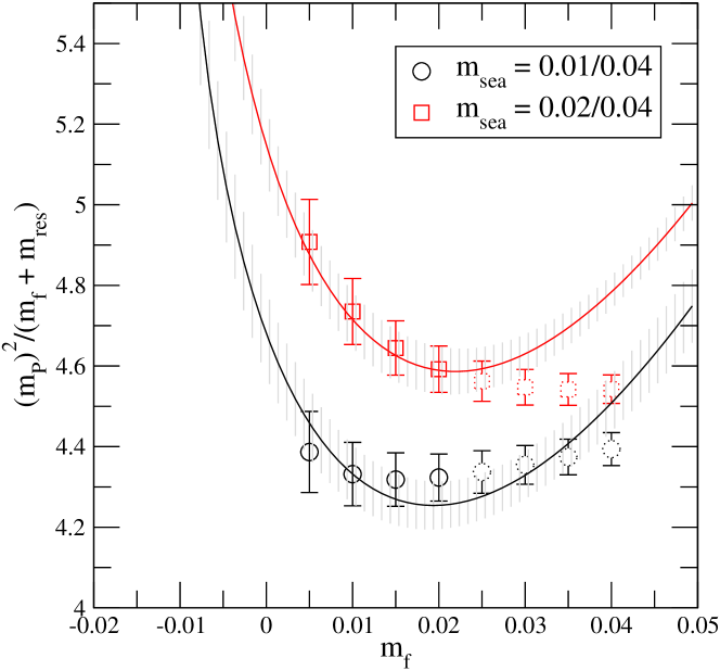
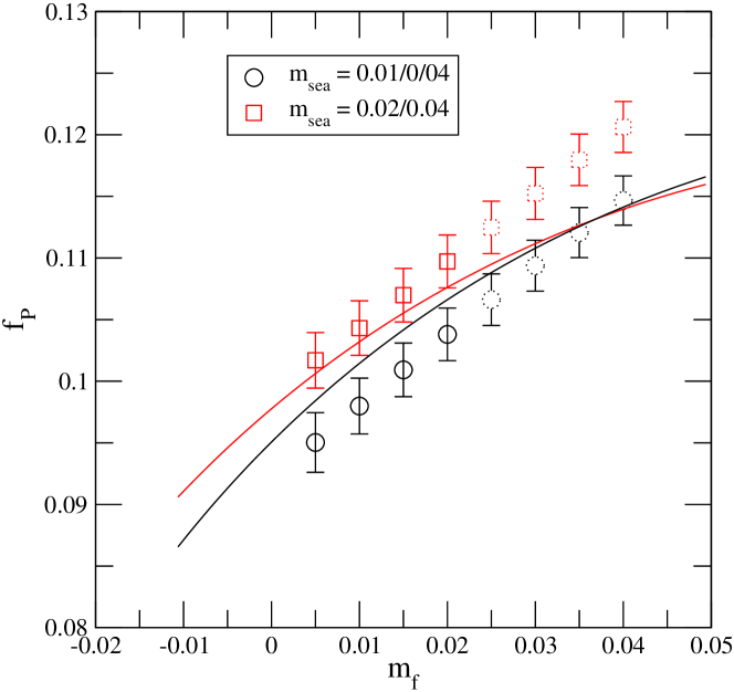
At NLO in PQ$\chi$PT the quark mass dependence of the pseudoscalar meson mass and decay constant has both a linear and non-linear component. For the lightest two DBW2 $\beta=0.72$ ensembles we have generated non-degenerate data for these two quantities, detailed in sections III.3 and III.5. Consequently, we can attempt fits to NLO partially quenched chiral formula to this data. A preliminary study of these fits was first reported in Lin:2005gh where $m_{P}$ and $f_{P}$ were fitted to the chiral formula independently. Here we update the results by performing combined fits to both $m_{P}$ and $f_{P}$. While we observed consistency between PQ$\chi$PT and our data with valence quark masses as heavy as 0.03 in the independent fits of  Lin:2005gh , this is not the case for the combined fits, shown in Figure 23 and 24. The fitted curves miss the data points badly at large quark masses. This is likely due to the fact that the quark masses are so heavy that the next-to-next-to-leading order contribution becomes important. Given the limited statistics, large residual mass, relatively small volume and coarse lattice spacing, our study on the chiral fits is far from conclusive. Further investigations on these lattice artifacts are in progress Lin:2006cf .

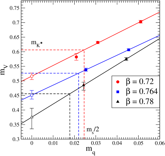
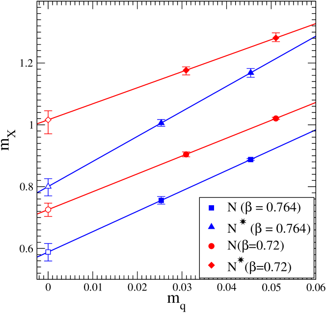
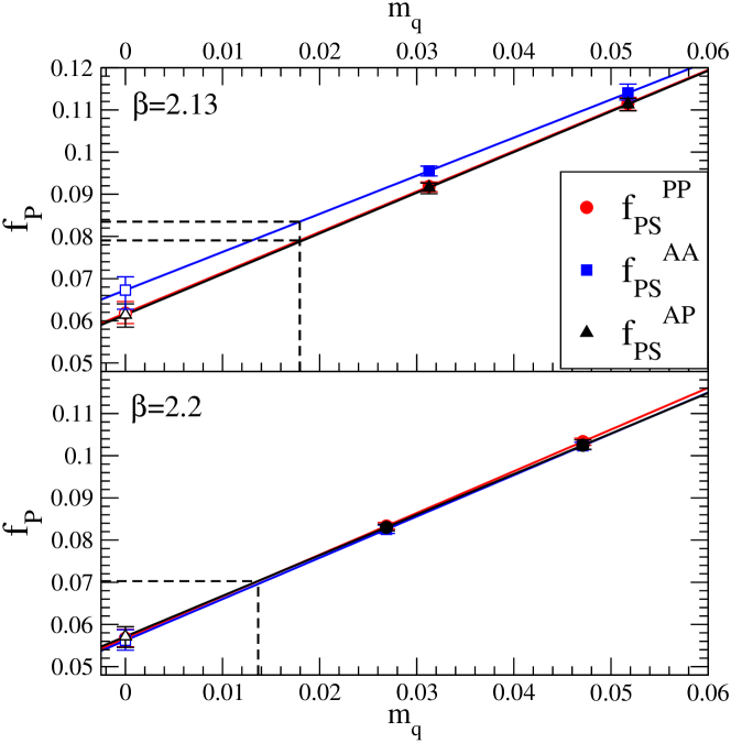
For all the RHMC datasets, we extrapolate linearly in quark mass ($m_{q}$), the unitary data for the quantity $m_{X}$ as follows

$$m_{X}(m_{q})=A_{X}+B_{X}m_{q}\ ,$$ (54)

where $m_{X}=\{m_{P}^{2},m_{V},m_{N},m_{N^{\star}},f_{P}\}$. Examples of these extrapolations for various datasets are shown in figures 25-28.

To predict physical quantities our strategy is as follows: The $u$ and $d$ quark masses are set to zero, and the lattice spacing is determined, either from $r_{0}$ or by setting the vector meson mass in this limit to be equal to that of the physical rho meson. The $s$ quark mass is then set from the physical kaon mass in lattice units and the pseudoscalar meson mass made from two quarks each with a mass of half the strange quark mass. Predictions for the values of the following quantities can then be made: $\{m_{K^{\star}},m_{N},m_{N^{\star}},f_{\pi},f_{K}\}$. Preliminary results were first presented in Antonio:2005jm ; Antonio:2005yh .

The results for the value of the vector meson in the chiral limit are listed in Table 22. The lattice spacing can then be determined from the physical rho meson mass. Whilst not ideal, as the rho meson can decay in nature and has a large width, and because we should extrapolate our data to the $u$ and $d$ quark masses, not the chiral limit, this method should be accurate enough for our purposes. The values of the lattice spacing determined in this way are also displayed in Table 22. One can compare these values for the lattice spacings with those obtained from the potential by setting $r_{0}=0.5$ fm, in Table 7. There is crude agreement, but the lattice spacing from the potential is systematically finer. Alternatively, we can estimate the value of $r_{0}$ from the potential and the lattice spacing determined from vector meson mass. This is also displayed in Table 22, where the errors quoted have been obtained by adding the errors for $r_{0}/a$ and $a^{-1}$ from the vector in quadrature. A crude estimate for the value of $r_{0}$ in the continuum can be made by an average, weighted by the square of the errors:

$$r_{0}=0.554(21)\ {\rm fm}.$$ (55)

This is equivalent to a constant continuum extrapolation and ignores the different systematic uncertainties for each ensemble, as well as the issues described above for extrapolation of the vector meson mass, and so should be only considered as a qualitative, rather than quantitative result. The determinations of the lattice spacing from the potential and the vector meson mass are consistent, given the uncertainty in the physical value of $r_{0}$. In general, despite its problematic nature, we used the vector meson mass to set the scale, where physical units were required and $r_{0}$ for scaling analyses as the value of $r_{0}/a$ is properly controlled for each ensemble.

For the larger rectangle data, where only valence chiral extrapolations are possible, we set the lattice spacing from the vector meson mass. The results are displayed in Table 23. Extrapolating $m_{V}$ with respect to the dynamical mass instead of the valence mass will decrease the value of $am_{\rho}$ by 10% to 15%, and hence increase the value of $a^{-1}$ by the same percentage. However, this is likely to effect all four datasets by a similar amount, so the valence chiral $m_{V}$ is good enough to compare the relative lattice spacings. We see that they are approximately matched, making the comparison of the residual mass meaningful.

The approximate value for the bare $s$ quark mass is extracted by requiring that a pseudoscalar meson made up of two quarks of mass $m_{s}/2$ has the experimental kaon mass. In doing this, we are neglecting both next-to-leading order chiral perturbation theory effects and the masses of the $u$ and $d$ quarks. Table 24 collects together the intercepts for the linear extrapolations, plus the extracted strange quark masses. These chiral extrapolations were performed on the multiple correlator fits tabulated in Table 8. As can be seen, the canonical heavy dynamical quark mass we have been using (0.04) is very close to the value of the $s$ quark mass extracted from this method.

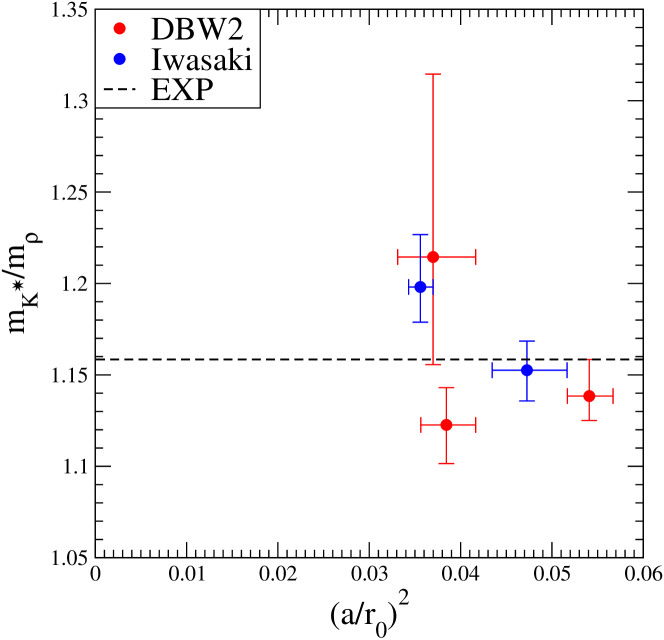
The values for $K^{\star}$, the nucleon and its negative parity partner are shown in Table 25. The determination of $m_{K^{\star}}$ can be seen for the DBW2 ensembles in Figure 26. We examined the scaling behaviour of dimensionless ratios versus $(a/r_{0})^{2}$. For the vector masses, this ratio was $m_{K^{\star}}/m_{\rho}$ and is shown in Figure 29. Given the change in lattice volumes, the relatively large values of residual mass, and only two sea-quark masses, the scaling behaviour appears reasonable.

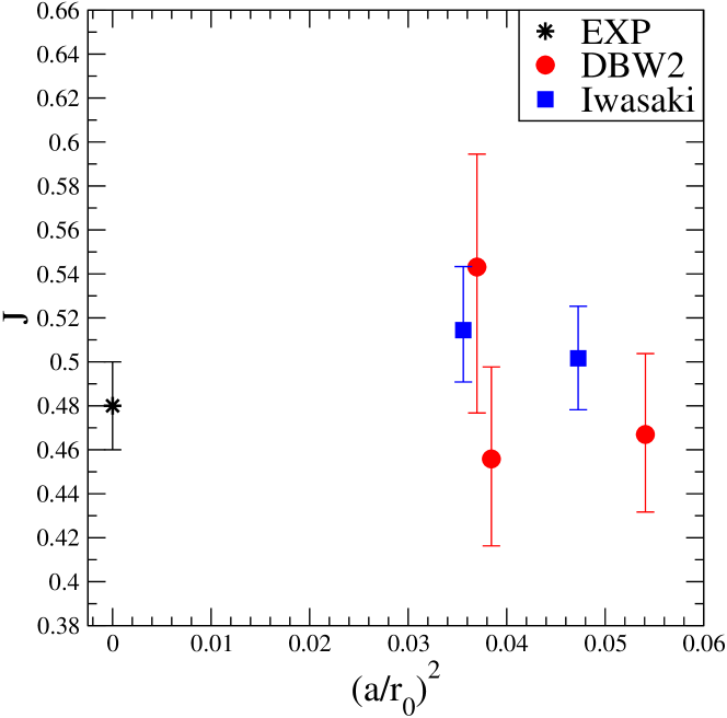
The $J$ parameter Lacock:1995tq is defined as

$$J=m_{V}\frac{dm_{V}}{dm_{P}^{2}}$$ (56)

and is determined at the experimental ratio

$$\frac{M_{K^{*}}}{M_{K}}=1.8.$$ (57)

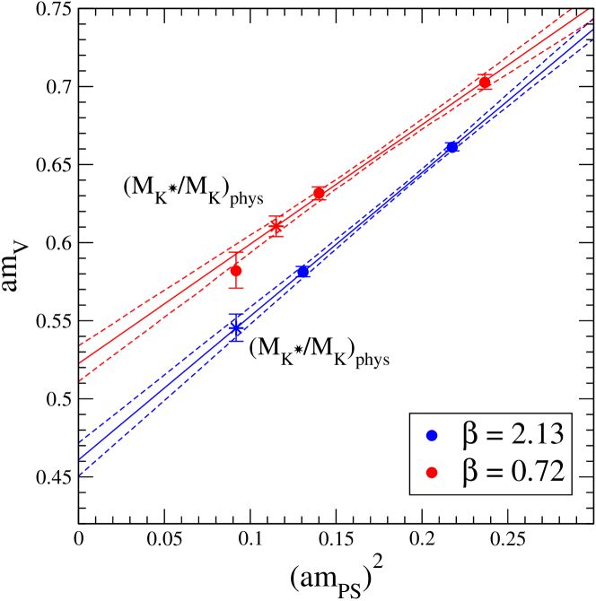
The linear fitting forms for the chiral extrapolations of the vector ($m_{V}$) and pseudoscalar ($m_{P}$) masses implying that a plot of $m_{V}$ versus $m_{P}^{2}$ will be a straight line for varying quark masses. Here we are working along the ‘unitary trajectory’ where $m_{\rm{sea}}=m_{\rm{val}}$. Figure 30 shows a plot of $m_{V}$ versus $m_{P}^{2}$ for the DBW2 $\beta$=0.72 and Iwasaki $\beta$=2.13 cases and, indeed, for the $\beta$ =0.72 case, where there are three points, approximate linear behaviour is seen. The intersection of this line with $m_{V}=1.8m_{S}$ (starred points) determines the reference value $m_{V}$ which is to be multiplied by the slope to yield $J$. Figure 31 shows the value of the $J$ parameter on all the datasets. Within the large errors, agreement with the experimental value is observed.

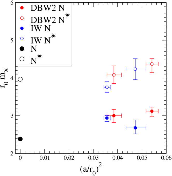
Figure 32 shows the dependence of the baryon spectrum at the chiral limit, in dimensionless units, on the lattice spacing. As the size of lattice is fixed to be $16^{3}\times 32$, the physical extent of the box in fm is smaller for the smaller $(a/r_{0})^{2}$ in Figure 32. The scaling behaviour of the spectrum appears promising despite the change in volume. A continuum extrapolation is not attempted. The $N^{\star}$ mass at the finest lattice spacings is approximately two sigma smaller than that at the coarsest lattice spacing, which is consistent with the theoretical expectation that the $N^{\star}$ becomes degenerate with the $N$ in a small enough box Sasaki:2001nf . This would also suggest that finite size effects may be beginning to affect the $N$ for the finest ensembles. These finite size effects would tend to increase the mass of the $N$ Fukugita:1992jj . With the current statistical resolution it is not possible to judge whether this is really the case.

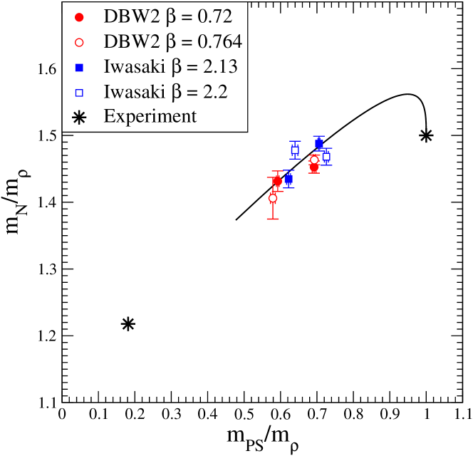
The Edinburgh plot Bowler:1985hr is shown in Figure 33. This is a useful way of comparing results for different actions without the need for any extrapolations of the data. Shown on the graph are the experimental ratios and the values obtained in the static quark limit, where the hadron mass is equal to the sum of the valence quark masses. The curve obtained from the phenomenological model for the hadron masses described in Ono:1977ss is shown as a guide for the eye. It is remarkable that, even at relatively coarse lattice spacing, with a small fifth dimension and moderate chiral symmetry breaking, the data follows the phenomenological curve, albeit with relatively large statistical error. This very promising result suggests that a reliable chiral extrapolation could be performed with more data.

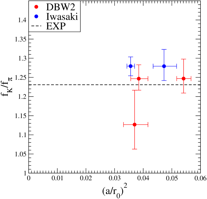
The values of the pseudoscalar meson decay constant in the chiral limit for all datasets are displayed in Table 26. Setting this equal to the physical value of $f_{\pi}$ provides another estimate of the lattice spacing. This is also tabulated in Table 26. The different methods for extracting the decay constant give consistent answers. For the Iwasaki $\beta=2.13$ data set, the $AA$ correlator gives slightly higher values than the other methods. However, at weaker coupling all the definitions agree, perhaps suggesting that this effect is a lattice artefact. Figure 34 shows the scaling behaviour of the dimensionless ratio $f_{K}/f_{\pi}$ from the $PP$ method. This shows excellent scaling, albeit with large errors and, moreover, is in agreement with the experimental value.

IV Conclusions

Our criteria to be able to simulate 2+1-flavor QCD on QCDOC using domain wall fermions are as follows. The topological charge autocorrelation length should not be significantly greater than one hundred HMC trajectories. Too infrequent changes in topological charge, particularly on the small lattices we are using, would signal poor ergodicity. On the other hand, the greater the presence of dislocations which drive topological change, the larger the density of localised near-zero modes which contribute to $m_{\rm res}$. To reach the chiral regime under theoretical control $m_{\mbox{\tiny res}}$ has to be small compared to the explicit $u$ and $d$ quark masses. Thus, a balance has to be struck between increasing the rate of local topological fluctuations and decreasing $m_{\rm res}$, i.e. the level of chiral symmetry breaking. Finally, to control both lattice artefacts and finite volume effects for light hadron physics, we need to simulate at lattice spacings in the range 0.09-0.13 fm and spatial extent of at least 2.5-3 fm.

We find the Iwasaki action satifies all these criteria. While the DBW2 gauge action produces a smaller $m_{\mbox{\tiny res}}$ at a given lattice spacing, we find the sampling of topological charge, especially at the finer lattice spacing to be too slow. Increasing the coefficient of the rectangle further produces only a modest decrease in $m_{\mbox{\tiny res}}$, while further supressing topology change.

We have presented results for the the static interquark potential, light meson and baryon masses, and light pseudoscalar decay contants. We find that, even on our small volumes and small extent in the 5th dimension, with rather heavy sea-quark masses and crude approach to chiral extrapolation, both the Iwasaki and DBW2 actions, reproduce experimental values, albeit with large statistical uncertainties. The scaling behavior appears promising over the range of lattice spacings from 0.09-0.13 fm, except for the baryons, where it appears to be spoiled by finite size effects for the smallest volume.

We conclude that, using the Iwasaki gauge action, there is a range of values for the quark masses and lattice spacings such that the chiral regime for 2+1 flavor QCD with domain wall fermions on QCDOC is accessible, while maintaining control of lattice artefacts and finite volume effects for a range of light hadron physics.

Table 1: 2+1-flavor ensembles and the mnemonics used to describe them. A $\star$ denotes that the ensemble was obtained by farming. A ${\dagger}$ denotes that the ensemble was farmed from a thermalised $R$ algorithm dataset. We generate $N_{\rm therm}$ trajectories (of length $\tau=1/2$) and a total of $N_{\rm traj}$ trajectories for each ensemble.

Action	$\beta$		$\frac{m_{l}}{m_{s}}$	Alg.	$\delta\tau$	Mnemonic	$N_{\rm traj}$	$N_{\rm therm}$
DBW2	0.	72	0.01/0.04	RHMC	$\frac{1}{50}$	(D, 0.72, 0.01/0.04)	6000	1000
DBW2	0.	72	0.02/0.04	RHMC	$\frac{1}{54}$	(D, 0.72, 0.02/0.04)	6000	1000
DBW2	0.	72	0.04/0.04	RHMC	$\frac{1}{50}$	(D, 0.72, 0.04/0.04)	3395	1600
DBW2⋆	0.	764	0.02/0.04	RHMC	$\frac{1}{70}$	(D, 0.764, 0.02/0.04)	2940	800
DBW2⋆†	0.	764	0.04/0.04	RHMC	$\frac{1}{70}$	(D 0.764, 0.04/0.04)	5320	100
DBW2	0.	78	0.02/0.04	RHMC	$\frac{1}{70}$	(D, 0.78 , 0.02/0.04)	1505	800
DBW2	0.	78	0.04/0.04	RHMC	$\frac{1}{70}$	(D, 0.78 , 0.04/0.04)	1620	800
Iwasaki	2.	13	0.02/0.04	RHMC	$\frac{1}{50}$	(I, 2.13 , 0.02/0.04)	3595	1000
Iwasaki	2.	13	0.04/0.04	RHMC	$\frac{1}{50}$	(I, 2.13 , 0.04/0.04)	3595	1000
Iwasaki	2.	2	0.02/0.04	RHMC	$\frac{1}{50}$	(I, 2.2 , 0.02/0.04)	5900	800
Iwasaki⋆	2.	2	0.04/0.04	RHMC	$\frac{1}{50}$	(I, 2.2 , 0.04/0.04)	5800	800

Table 2: 2+1-flavor datasets used in our exploration of gauge actions with different plaquette and rectangle contributions and the ensemble mnemonics we use to describe them. The top three datasets have the same lattice spacing, and the others are finer. Here MD time refers to Molecular Dynamics evolution time.

$c_{1}$		$\beta$		$\frac{m_{l}}{m_{s}}$	Alg.	$\delta\tau$	Mnemonic	MD time	$N_{\rm therm}$
-2.	3	0.	48	0.04/0.04	R	0.01	(C2.3, 0.48, 0.04/0.04, R)	800	300
-3.	57	0.	32	0.04/0.04	R	0.01	(C3.57, 0.32, 0.04/0.04, R)	800	300
-7.	47	0.	16	0.04/0.04	R	0.01	(C7.47, 0.16, 0.04/0.04, R)	760	300
-3.	57	0.	333	0.04/0.04	R	0.01	(C3.57, 0.33, 0.04/0.04, R)	760	300
-3.	57	0.	36	0.04/0.04	R	0.01	(C3.57, 0.36, 0.04/0.04, R)	690	300
-2.	3	0.	53	0.04/0.04	R	0.01	(C2.3, 0.53, 0.04/0.04, R)	700	300

Table 3: Parameter values for the 2+1 flavour RHMC algorithm simulations. $\lambda_{\rm min}$ and $\lambda_{\rm max}$ are the maximum and minimum eigenvalues of ${\cal D}(m_{i})$, which are needed for the rational approximation. $n_{\rm MD}$ is the degree of the rational approximation used in the molecular dynamics evolution and $n_{\rm MC}$ is the rational approximation degree used in the Monte Carlo accept/reject step. The conjugate gradient stopping condition for the evolution was $1.0\times 10^{-6}$ and for the accept/reject step was $1.0\times 10^{-10}$.

Ensemble		$m_{l}$			$m_{s}$			$m_{PV}$
	$\lambda_{\rm max}$	$\lambda_{\rm min}$	$n_{\rm MD}$	$n_{\rm MC}$	$\lambda_{\rm min}$	$n_{\rm MD}$	$n_{\rm MC}$	$\lambda_{\rm min}$	$n_{\rm MD}$	$n_{\rm MC}$
(D, 0.72, 0.01/0.04)	2.4	$6\times 10^{-5}$	11	18	$6\times 10^{-4}$	9	14	$4\times 10^{-2}$	6	9
(D, 0.72, 0.02/0.04)	2.4	$2\times 10^{-4}$	10	15	$4\times 10^{-4}$	9	14	$3\times 10^{-2}$	6	9
(D, 0.72, 0.04/0.04)	2.4	$6\times 10^{-4}$	9	14	$6\times 10^{-4}$	9	14	$3\times 10^{-2}$	6	9
(D, 0.764, 0.02/0.04)	2.42	$1\times 10^{-4}$	10	15	$3\times 10^{-4}$	9	14	$2\times 10^{-2}$	5	8
(D, 0.764, 0.04/0.04)	2.42	$1\times 10^{-4}$	10	15	$3\times 10^{-4}$	9	14	$2\times 10^{-2}$	5	8
(D, 0.78, 0.02/0.04)	2.42	$1\times 10^{-4}$	10	15	$3\times 10^{-4}$	9	14	$2\times 10^{-2}$	5	8
(D, 0.78, 0.04/0.04)	2.42	$1\times 10^{-4}$	10	15	$3\times 10^{-4}$	9	14	$2\times 10^{-2}$	5	8
(I, 2.13, 0.02/0.04)	2.4	$1\times 10^{-4}$	10	15	$3\times 10^{-4}$	9	14	$3\times 10^{-2}$	5	8
(I, 2.13, 0.04/0.04)	2.4	$1\times 10^{-4}$	10	15	$3\times 10^{-4}$	9	14	$3\times 10^{-2}$	5	8
(I, 2.2, 0.02/0.04)	2.4	$2\times 10^{-4}$	10	15	$4\times 10^{-4}$	9	14	$3\times 10^{-2}$	5	8
(I, 2.2, 0.04/0.04)	2.4	$2\times 10^{-4}$	10	15	$4\times 10^{-4}$	9	14	$3\times 10^{-2}$	5	8

Table 4: Statistics for 2+1 flavour DBW2 ensembles with $\beta=0.72$ generated with the RHMC algorithm.

Ensemble	$<\delta H>$	$<e^{-\delta H}>$	Accept	$\overline{P_{\mu\nu}}$	$\langle\bar{q}q\rangle$		$\langle\bar{q}\gamma_{5}q\rangle\times 10^{-5}$
(D, 0.72, 0.01/0.04)	0.388(14)	0.991(14)	0.658(6)	0.608201(21)	0.00315(	1)	4.	7(145)
(D, 0.72, 0.02/0.04)	0.311(13)	1.000(15)	0.693(5)	0.608094(18)	0.00422(	9)	9.	6(7.9)
(D, 0.72, 0.04/0.04)	0.398(16)	0.992(15)	0.651(9)	0.607788(10)	0.00612(	11)	-0.	6(8.4)

Table 5: Estimates of autocorrelation times for the average plaquette and the pseudoscalar meson on timeslice 12. Note plaquettes are separated by 1 trajectory while pseudoscalar meson correlators are measured on $N_{\rm meas}$ configurations each separated by 5 trajectories.

Dataset	Ensemble size		$\langle P_{\mu,\nu}\rangle$		$C_{P}(t=12)$
($\beta:\frac{m_{l}}{m_{s}}$)	$N_{\rm traj}$	$N_{\rm meas}$	$\tau^{\rm cum}$	$\tau^{\rm exp}$	$\tau^{\rm cum}$	$\tau^{\rm exp}$
(D, 0.72 , 0.01/0.04)	6000	1000	$20(10)$	$>4$	$13(10)$	$>8$
(D, 0.72 , 0.02/0.04)	6000	1000	$10(5)$	$>5$	$15(10)$	$>12$
(I, 2.13 , 0.02/0.04)	3595	520	$6(3)$	$>6$	$5(3)$	$>5$
(I, 2.13 , 0.04/0.04)	3595	520	$6(4)$	$>4$	$7(3)$	$>9$

Table 6: Results for the coefficients appearing in the fit to the static quark potential given in Eq. (16) and the implied values of $r_{0}$ and $1/a$. In computing the latter, the value $r_{0}=0.5$fm is used. The configurations used to obtain the results in this table are separated by 5 Monte Carlo steps.

Ensemble Mnemonic	$N_{\rm meas}$	$V_{0}$		$\alpha$		$\sigma$		$r_{0}$		$1/a$ GeV
(D, 0.72, 0.01/0.04)	900	0.	880(10)	0.	466(13)	0.	0754(19)	3.	962(30)(16)	1.	564(12)(6)
(D, 0.72, 0.02/0.04)	800	0.	853(11)	0.	434(13)	0.	0817(21)	3.	858(32)(75)	1.	523(13)(30)
(D, 0.72, 0.04/0.04)	280	0.	783(17)	0.	365(22)	0.	1018(32)	3.	554(31)(67)	1.	403(12)(27)
(D, 0.764, 0.02/0.04)	294	0.	816(20)	0.	417(27)	0.	0571(33)	4.	646(84)(21)	1.	833(33)(08)
(D, 0.764, 0.04/0.04)	300	0.	793(19)	0.	398(26)	0.	0648(31)	4.	397(60)(18)	1.	735(24)(07)
(D, 0.78 , 0.02/0.04)	180	0.	791(9)	0.	412(11)	0.	0524(16)	4.	863(54)(142)	1.	929(21)(56)
(D, 0.78 , 0.04/0.04)	165	0.	761(10)	0.	378(13)	0.	0601(18)	4.	600(49)(16)	1.	815(19)(6)
(I, 2.13 , 0.02/0.04)	420	0.	834(10)	0.	406(13)	0.	0668(18)	4.	315(41)(97)	1.	703(16)(38)
(I, 2.13 , 0.04/0.04)	240	0.	792(14)	0.	350(18)	0.	0770(25)	4.	110(41)(21)	1.	622(16)(8)
(I, 2.2 , 0.02/0.04)	280	0.	804(7)	0.	393(9)	0.	0506(12)	4.	982(45)(30)	1.	966(18)(23)
(I, 2.2 , 0.04/0.04)	320	0.	781(6)	0.	365(9)	0.	0560(11)	4.	788(35)(30)	1.	890(14)(12)
(I, 2.3 , 0.04/0.04)	165	0.	741(5)	0.	348(8)	0.	0397(9)	5.	729(55)(137)	2.	261(22)(54)
(C2.3, 0.48 , 0.04/0.04, R)	180	0.	814(16)	0.	413(19)	0.	0773(32)	4.	002(57)(60)	1.	579(22)(24)
(C2.3, 0.53 , 0.04/0.04, R)	160	0.	739(6)	0.	384(8)	0.	0492(12)	5.	074(48)(48)	2.	002(19)(19)
(C3.57, 0.32 , 0.04/0.04, R)	180	0.	828(15)	0.	433(18)	0.	0773(28)	3.	968(49)(43)	1.	566(19)(17)
(C3.57, 0.33 , 0.04/0.04, R)	145	0.	792(12)	0.	416(15)	0.	0657(21)	4.	335(47)(102)	1.	711(19)(40)
(C3.57, 0.36 , 0.04/0.04, R)	135	0.	719(9)	0.	371(12)	0.	0500(17)	5.	060(66)(33)	1.	997(26)(13)
(C7.47, 0.16 , 0.04/0.04, R)	165	0.	832(15)	0.	448(19)	0.	0733(30)	4.	050(57)(430)	1.	598(22)(17)

Table 7: Results for the lattice spacing extrapolated to the chiral limit for the two light quarks, $m_{f}=-m_{\rm res}$, while the mass of the third (strange) quark is held fixed at $m_{f}=0.04$. The masses column lists those sea quark masses used in the extrapolation.

Action	$\beta$		masses	$r_{0}$	$1/a$ [GeV]
DBW2	0.	72	0.01, 0.02, 0.04	4.260(52)(12)	1.681(20)(5)
DBW2	0.	72	0.01, 0.02	4.177(115)(105)	1.648(41)(45)
DBW2	0.	764	0.02, 0.04	5.030(230)(040)	1.983(92)(16)
DBW2	0.	78	0.02, 0.04	5.184(134)(335)	2.046(53)(132)
Iwasaki	2.	13	0.02, 0.04	4.628(121)(239)	1.826(48)(94)
Iwasaki	2.	20	0.02, 0.04	5.239(114)(111)	2.068(44)(45)

Table 8: Results for pseudoscalar meson masses from fits to unitary RHMC data.

Ensemble Mnemonic	Fit range	Results
	$t_{\rm min}-t_{\rm max}$	$m_{\rm{val}}$	$m_{P}$	$\chi^{2}/dof$	correlators
(D, 0.72 , 0.1/0.04)	4-14	0.01	$0.303(3)$	$66/16$	SL-SL, SS-SS
(D, 0.72 , 0.02/0.04)	5-16	0.02	$0.3742(9)$	$34/18$	LL-LL, WL-WL
(D, 0.72 , 0.04/0.04)	5-16	0.04	$0.4916(10)$	$50/18$	LL-LL, WL-WL
(D, 0.764 , 0.02/0.04)	7-15	0.02	$0.311(1)$	$20/12$	LL-LL, WL-WL
(D, 0.764 , 0.04/0.04)	6-16	0.04	$0.4203(7)$	$23/16$	LL-LL, WL-WL
(D, 0.78 , 0.02/0.04)	11-16	0.02	$0.288(6)$	$5/4$	WL-WL
(D, 0.78 , 0.04/0.04)	11-16	0.04	$0.400(7)$	$8/4$	LL-LL
(I, 2.13 , 0.02/0.04)	10-16	0.02	$0.362(2)$	$10/8$	LL-LL, SL-SL
(I, 2.13 , 0.04/0.04)	9-16	0.04	$0.4665(9)$	$14/10$	SL-SL, SS-SS
(I, 2.2 , 0.02/0.04)	5-16	0.02	$0.315(2)$	$29/18$	LL-LL, WL-WL
(I, 2.2 , 0.04/0.04)	6-16	0.04	$0.425(1)$	$21/16$	LL-LL, WL-WL

Table 9: Results for pseudoscalar meson masses from fits to non-degenerate LL-LL DBW2 $\beta=0.72$ RHMC data.

$m_{\rm val}$	Fit range	$m_{l}$
	$t_{\rm min}-t_{\rm max}$	0.01	0.02	0.04
0.005	8-16	$0.2619(26)$	$0.2769(30)$
0.01	8-16		$0.3125(27)$
0.015	8-16	$0.3321(23)$	$0.3450(25)$
0.02	8-16	$0.3627(22)$		$0.3882(17)$
0.025	8-16	$0.3914(21)$	$0.4031(22)$
0.03	8-16	$0.4186(21)$	$0.4298(21)$	$0.4419(16)$
0.035	8-16	$0.4445(20)$	$0.4552(20)$
0.04	8-16	$0.4693(20)$	$0.4795(19)$

Table 10: Results for the vector meson masses from fits to unitary RHMC data.

Ensemble Mnemonic	Fit range	Results
	$t_{\rm min}-t_{\rm max}$	$m_{V}$	$\chi^{2}/dof$	correlators
(D, 0.72 , 0.01/0.04)	6-14	$0.580(10)$	$13/12$	LL-LL,SL-SL
(D, 0.72 , 0.02/0.04)	6-16	$0.635(4)$	$27/16$	LL-LL,WL-WL
(D, 0.72 , 0.04/0.04)	6-13	$0.703(5)$	$11/10$	LL-LL,WL-WL
(D, 0.764 , 0.02/0.04)	8-14	$0.543(5)$	$13/8$	LL-LL,WL-WL
(D, 0.764 , 0.04/0.04)	7-15	$0.607(3)$	$21/12$	LL-LL,WL-WL
(D, 0.78 , 0.02/0.04)	10-15	$0.48(3)$	$2/4$	WL-WL
(D, 0.78 , 0.04/0.04)	8-15	$0.575(5)$	$24/13$	LL-LL,WL-WL
(I, 2.13 , 0.02/0.04)	5-14	$0.581(4)$	$14/8$	SS-SS
(I, 2.13 , 0.04/0.04)	6-14	$0.661(3)$	$21/12$	SS-SS,SL-SL
(I, 2.2 , 0.02/0.04)	7-16	$0.493(6)$	$11/14$	LL-LL,WL-WL
(I, 2.2 , 0.04/0.04)	7-15	$0.586(5)$	$19/12$	LL-LL,WL-WL

Table 11: Results for the vector meson masses from fits to non-degenerate LL-LL DBW2 $\beta=0.72$ RHMC data.

$m_{\rm val}$	Fit range	$m_{l}$
	$t_{\rm min}-t_{\rm max}$	0.01	0.02	0.04
0.005	8-16	$0.574(22)$	$0.586(18)$
0.01	8-16		$0.596(15)$
0.015	8-16	$0.595(13)$	$0.610(13)$
0.02	8-16	$0.610(11)$		$0.648(12)$
0.025	8-16	$0.6258(90)$	$0.6405(97)$
0.03	8-16	$0.6419(78)$	$0.6564(87)$	$0.6744(94)$
0.035	8-16	$0.6579(69)$	$0.6723(78)$
0.04	8-16	$0.6740(62)$	$0.6880(71)$

Table 12: Results for the nucleon and negative parity partner from fits to the unitary RHMC data.

Dataset	$t_{\rm min}-t_{\rm max}$			Results
Ensemble	$N$ from $\Omega_{B_{1}}$	$N^{\star}$ from $\Omega_{B_{1}}$	$N^{\star}$ from $\Omega_{B_{2}}$	$m_{N}$	$m_{N^{\star}}$	$\chi^{2}/dof$
(D, 0.72 , 0.02/0.04 )	10-16	20-27	6-11	$0.904(8)$	$1.18(2)$	$26/16$
(D, 0.72 , 0.04/0.04 )	8-14	23-25	4-8	$1.021(4)$	$1.28(2)$	$13/10$
(D, 0.764 , 0.02/0.04 )	11-15	20-23	6-10	$0.76(2)$	$0.96(2)$	$16/9$
(D, 0.764 , 0.04/0.04 )	10-16	20-23	7-12	$0.888(3)$	$1.17(1)$	$23/12$
( I, 2.13 , 0.02/0.04 )	9-14	21-25	7-9	$0.82(1)$	$1.14(2)$	$11/9$
( I, 2.13 , 0.04/0.04 )	8-12	24-25	6-11	$0.984(5)$	$1.28(2)$	$8/8$
( I, 2.2 , 0.02/0.04 )	8-16	21-25	6-10	$0.729(3)$	$0.90(1)$	$15/14$
( I, 2.2 , 0.04/0.04 )	10-15	21-26	6-11	$0.860(4)$	$1.051(5)$	$19/13$

Table 13: Results for the residual mass for unitary data on the RHMC data.

Ensemble Mnemonic	Fit range	Results
	$t_{\rm min}-t_{\rm max}$	$m^{\prime}_{\rm res}(m_{f})$	$\chi^{2}/dof$
(D, 0.72 , 0.01/0.04)	5-16	$0.01089(4)$	$51/11$
(D, 0.72 , 0.02/0.04)	9-16	$0.01092(7)$	$18/15$
(D, 0.72 , 0.04/0.04)	8-16	$0.01146(8)$	$31/15$
(D, 0.764 , 0.02/0.04)	9-15	$0.00535(2)$	$18/13$
(D, 0.764 , 0.04/0.04)	10-14	$0.00540(1)$	$12/9$
(D, 0.78 , 0.02/0.04)	11-15	$0.00428(2)$	$6/4$
(D, 0.78 , 0.04/0.04)	4-15	$0.00427(2)$	$9/11$
(I, 2.13 , 0.02/0.04)	10-15	$0.01127(3)$	$12/11$
(I, 2.13 , 0.04/0.04)	9-15	$0.01175(5)$	$20/13$
(I, 2.2 , 0.02/0.04)	10-15	$0.00688(2)$	$19/11$
(I, 2.2 , 0.04/0.04)	12-16	$0.00711(2)$	$17/9$

Table 14: Results for the residual mass, $m^{\prime}_{\rm res}(m_{f})$ for the LL non-degenerate DBW2 $\beta=0.72$ RHMC data.

$m_{l}^{\rm val}$	$m_{l}^{\rm dyn}=0.01$	$m_{l}^{\rm dyn}=0.02$	$m_{l}^{\rm dyn}=0.04$
0.005	0.01101(6)	0.01120(7)
0.010		0.01109(7)
0.015	0.01078(5)	0.01097(6)
0.020	0.01068(5)		0.01191(10)
0.025	0.01059(5)	0.01077(6)
0.030	0.01050(5)	0.01068(6)	0.01167(9)
0.035	0.01042(5)	0.01060(6)
0.040	0.01035(5)	0.01053(6)

Table 15: The vector meson masses and the residual masses computed for the four data sets: (D, 0.72, 0.04/0.04, R), (C2.3, 0.48, 0.04/0.04, R), (C3.57, 0.32, 0.04/0.04, R), and (C7.47, 0.16, 0.04/0.04, R).

Ensemble	$m_{\rm val}$	$m_{V}$	$m^{\prime}_{\rm res}(m_{f})$
(D, 0.72, 0.04/0.04, R)	$0.02$	$0.626(10)$	$0.01141(6)$
	$0.03$	$0.655(8)$	$0.01119(6)$
	$0.04$	$0.685(7)$	$0.01100(5)$
	$0.05$	$0.715(6)$	$0.01084(5)$
(C2.3, 0.48, 0.04/0.04, R)	$0.02$	$0.612(10)$	$0.00781(6)$
	$0.03$	$0.636(10)$	$0.00768(5)$
	$0.04$	$0.661(8)$	$0.00756(5)$
	$0.05$	$0.689(6)$	$0.00747(4)$
(C3.57, 0.32, 0.04/0.04, R)	$0.02$	$0.598(11)$	$0.00754(5)$
	$0.03$	$0.628(9)$	$0.00742(5)$
	$0.04$	$0.657(8)$	$0.00732(5)$
	$0.05$	$0.686(7)$	$0.00723(4)$
(C7.47, 0.16, 0.04/0.04, R)	$0.02$	$0.599(10)$	$0.00654(5)$
	$0.03$	$0.623(8)$	$0.00642(5)$
	$0.04$	$0.650(7)$	$0.00634(4)$
	$0.05$	$0.678(6)$	$0.00626(4)$

Table 16: Results for $Z_{A}$ from fits to unitary RHMC data.

Ensemble Mnemonic	Fit range	Results
($\beta,m_{l}/m_{s}$)	$t_{\rm min}-t_{\rm max}$	$Z_{A}$	$\chi^{2}/dof$	correlators
( D, 0.72 , 0.01/0.04 )	5-11	$0.7335(2)$	$18/13$	SL-SL
( D, 0.72 , 0.02/0.04 )	5-11	$0.7347(2)$	$19/13$	SL-SL
( D, 0.72 , 0.04/0.04 )	8-13	$0.7373(1)$	$11/11$	SL-SL
( D, 0.764 , 0.02/0.04 )	6-12	$0.75521(5)$	$25/13$	WL-WL
( D, 0.764 , 0.04/0.04 )	6-14	$0.75722(7)$	$21/17$	WL-WL
( D, 0.78 , 0.02/0.04 )	8-14	$0.7625(3)$	$14/13$	WL-WL
( D, 0.78 , 0.04/0.04 )	8-14	$0.7662(2)$	$17/13$	WL-WL
( I, 2.13 , 0.02/0.04 )	7-14	$0.73376(10)$	$28/15$	SL-SL
( I, 2.13 , 0.04/0.04 )	6-11	$0.7357(1)$	$22/11$	SL-SL
( I, 2.2 , 0.02/0.04 )	10-15	$0.74563(9)$	$13/11$	WL-WL
( I, 2.2 , 0.04/0.04 )	10-15	$0.74820(7)$	$23/11$	WL-WL

Table 17: Results for $Z_{A}$ from fits to non-degenerate LL-LL DBW2 $\beta=0.72$ RHMC data.

$m_{\rm val}$	Fit range	$m_{l}$
	$t_{\rm min}-t_{\rm max}$	0.01	0.02	0.04
0.005	8-16	$0.73207(32)$	$0.73382(29)$
0.01	8-16		$0.73413(26)$
0.015	8-16	$0.73338(22)$	$0.73461(24)$
0.02	8-16	$0.73416(20)$		$0.73518(29)$
0.025	8-16	$0.73498(19)$	$0.73592(20)$
0.03	8-16	$0.73583(19)$	$0.73668(20)$	$0.73651(22)$
0.035	8-16	$0.73670(19)$	$0.73745(19)$
0.04	8-16	$0.73759(19)$	$0.73825(18)$

Table 18: Fitted values for the pseudoscalar meson decay constant using the value of $Z_{A}$ and the axial-axial correlator for unitary RHMC data, Eq. (40).

Dataset	Fit range	Results
	$t_{\rm min}-t_{\rm max}$	$A_{A_{0}A_{0}}$	$f_{P}$	$\chi^{2}/dof$
( D, 0.72 , 0.01/0.04 )	9-15	$0.028(2)$	$0.099(3)$	$9./6$
( D, 0.72 , 0.02/0.04 )	9-15	$0.044(1)$	$0.111(2)$	$11/6$
( D, 0.72 , 0.04/0.04 )	9-15	$0.075(3)$	$0.128(3)$	$11/6$
( D, 0.764 , 0.02/0.04 )	8-16	$0.0219(5)$	$0.0890(8)$	$14/7$
( D, 0.764 , 0.04/0.04 )	8-15	$0.043(1)$	$0.107(1)$	$8/6$
( D, 0.78 , 0.02/0.04 )	11-16	$0.016(2)$	$0.083(3)$	$9/4$
( D, 0.78 , 0.04/0.04 )	12-16	$0.026(2)$	$0.086(2)$	$5/4$
( I, 2.13 , 0.02/0.04 )	5-16	$0.0307(7)$	$0.096(1)$	$13/11$
( I, 2.13 , 0.04/0.04 )	10-16	$0.057(2)$	$0.114(2)$	$3/6$
( I, 2.2 , 0.02/0.04 )	9-16	$0.0195(5)$	$0.0825(10)$	$10/6$
( I, 2.2 , 0.04/0.04 )	10-16	$0.0407(7)$	$0.1024(9)$	$14/6$

Table 19: Fitted values for the pseudoscalar meson decay constant using the value of $Z_{A}$ and axial-axial correlator for non-degenerate DBW2 $\beta=0.72$ RHMC data, Eq. (40).

$m_{l}^{\rm val}$	$m_{l}^{\rm dyn}=0.01$	$m_{l}^{\rm dyn}=0.02$	$m_{l}^{\rm dyn}=0.04$
0.005	0.0950(24)	0.1017(23)
0.010		0.1043(22)
0.015	0.1009(22)	0.1070(22)
0.020	0.1038(21)		0.1213(29)
0.025	0.1066(21)	0.1125(21)
0.030	0.1094(21)	0.1152(21)	0.1260(28)
0.035	0.1121(20)	0.1180(21)
0.040	0.1147(20)	0.1206(21)

Table 20: Fitted values for the pseudoscalar meson decay constant using the residual mass and the pseudoscalar density correlator, Eq. (43) for the unitary RHMC data.

Dataset	Fit range	Results
	$t_{\rm min}-t_{\rm max}$	$A_{PP}$	$f_{P}$	$\chi^{2}/dof$
(D, 0.72 , 0.01/0.04 )	11-16	$0.76(5)$	$0.097(3)$	$18/5$
(D, 0.72 , 0.02/0.04 )	8-16	$0.93(3)$	$0.115(2)$	$7/8$
(D, 0.72 , 0.04/0.04 )	10-16	$0.96(4)$	$0.129(3)$	$9/5$
(D, 0.764 , 0.02/0.04 )	10-16	$0.49(1)$	$0.0884(9)$	$12/5$
(D, 0.764 , 0.04/0.04 )	11-16	$0.55(1)$	$0.108(1)$	$7/4$
(D, 0.78 , 0.02/0.04 )	11-16	$0.36(3)$	$0.080(3)$	$2/4$
(D, 0.78 0.04/0.04)	11-16	$0.35(2)$	$0.089(3)$	$6/4$
(I, 2.13 , 0.02/0.04 )	10-16	$0.53(2)$	$0.092(1)$	$8/5$
(I, 2.13 , 0.04/0.04 )	9-16	$0.60(2)$	$0.112(2)$	$7/7$
(I, 2.2 , 0.02/0.04 )	9-16	$0.39(1)$	$0.0833(8)$	$10/7$
(I, 2.2 , 0.04/0.04 )	11-16	$0.48(1)$	$0.1033(9)$	$8/4$

Table 21: Fitted values for the pseudoscalar meson decay constant using $Z_{A}$ and the local axial correlator, Eq. (47).

Dataset	Fit range	Results
	$t_{\rm min}-t_{\rm max}$	$f_{P}$	$\chi^{2}/dof$
( D, 0.72 , 0.01/0.04 )	10-16	$0.11(2)$	$1/6$
( D, 0.72 , 0.02/0.04 )	10-16	$0.113(2)$	$7/6$
( D, 0.72 , 0.04/0.04 )	12-16	$0.127(3)$	$5/4$
( D, 0.764 , 0.02/0.04 )	11-16	$0.089(1)$	$4/4$
( D, 0.764 , 0.04/0.04 )	11-16	$0.107(1)$	$6/4$
( D, 0.78 , 0.02/0.04 )	12-16	$0.076(3)$	$8/4$
( D, 0.78 , 0.04/0.04 )	10-16	$0.088(3)$	$0.3/5$
( I, 2.13 , 0.02/0.04 )	11-16	$0.092(1)$	$4/5$
( I, 2.13 , 0.04/0.04 )	10-16	$0.111(2)$	$3/5$
( I, 2.2 , 0.02/0.04 )	11-16	$0.0830(8)$	$7/5$
( I, 2.2 , 0.04/0.04 )	10-16	$0.102(1)$	$10/5$

Table 22: Vector meson masses in the chiral limit and $r_{0}$

Dataset	Results
dataset	$m_{V}$	$a^{-1}$ (GeV)	$\chi^{2}/dof$	$r_{0}$(fm)
(D,0.72)	$0.52^{+1}_{-1}$	$1.49^{+3}_{-3}$	$1/1$	0.564(13)
(D,0.764)	$0.45^{+2}_{-1}$	$1.71^{+5}_{-6}$	-	0.580(20)
(D,0.78)	$0.38^{+3}_{-4}$	$2.1^{+2}_{-2}$	-	0.487(57)
(I,2.13)	$0.46^{+1}_{-1}$	$1.68^{+4}_{-4}$	-	0.544(34)
(I,2.2)	$0.37^{+1}_{-2}$	$2.08^{+9}_{-6}$	-	0.497(28)

Table 23: Results for the residual mass and the vector meson masses with different rectangle contributions. The values shown are extrapolations to the valence chiral limit: $m_{val}=0$ for the residual masses and $m_{val}=-m_{\rm res}$ for vector meson masses. The inverse lattice spacings determined from the vector meson masses are shown in the last column.

Ensemble	$m^{\prime}_{\rm res}$	$m_{V}$	$1/a$ (GeV)
(D, 0.72, 0.04/0.04, R)	0.01176(7)	0.530(15)	1.450(41)
(C2.3, 0.48, 0.04/0.04, R)	0.00802(6)	0.539(16)	1.430(43)
(C3.57, 0.32, 0.04/0.04, R)	0.00773(6)	0.517(16)	1.489(45)
(C7.47, 0.16, 0.04/0.04, R)	0.00670(6)	0.525(16)	1.467(44)
(C3.57, 0.333, 0.04/0.04, R)	0.00480(9)	0.509(26)	1.51(8)
(C3.57, 0.36, 0.04/0.04, R)	0.002306(21)	0.400(12)	1.92(7)
(C2.3, 0.53, 0.04/0.04, R)	0.002683(30)	0.405(17)	1.90(8)

Table 24: Pseudoscalar meson mass squared in the chiral limit and the bare $s$ quark mass.

Ensembles	Results
	$m_{P}(m_{q}\rightarrow 0)$	$\chi^{2}/dof$	$m_{s}(m_{\rho})$
(D,0.72)	$-0.014(2)$	$0.006/1$	$0.049(2)$
(D,0.764)	$-0.004(2)$	-	$0.044(3)$
(D,0.78)	$-0.011(10)$	-	$0.036(5)$
(I,2.13)	$-0.002(4)$	-	$0.042(2)$
(I,2.2 )	$-0.008(3)$	-	$0.032(2)$

Table 25: Results for $m_{K^{\star}}$, the nucleon and its negative partity partner.

Dataset	$m_{K^{\star}}$	$m_{N}$	$m_{N^{\star}}$
(D,0.72)	$0.588(7)$	$0.73(2)$	$1.02(5)$
(D,0.764)	$0.51(1)$	$0.59(4)$	$0.80(3)$
(D,0.78)	$0.46(2)$	-	-
(D,2.13)	$0.529(10)$	$0.58(3)$	$0.92(5)$
(D,2.2)	$0.443(9)$	$0.554(9)$	$0.71(3)$

Table 26: Pseudoscalar meson decay constant in the chiral limit and corresponding lattice spacing from the physical value of $f_{\pi}$.

Dataset	Results
$\beta$	$f_{P}^{PP}$	$a^{-1}$ (GeV)	$f_{P}^{AA}$	$a^{-1}$ (GeV)	$f_{P}^{AP}$	$a^{-1}$ (GeV)
0.72	$0.080(5)$	$1.6(1)$	$0.082(4)$	$1.59(8)$	$0.082(4)$	$1.59(8)$
0.764	$0.064(2)$	$2.04(6)$	$0.067(2)$	$1.94(7)$	$0.065(3)$	$1.99(9)$
0.78	$0.068(8)$	$1.9(3)$	$0.07(1)$	$1.8(3)$	$0.062(8)$	$2.1(3)$
2.13	$0.062(3)$	$2.10(9)$	$0.067(5)$	$1.9(1)$	$0.061(3)$	$2.1(1)$
2.2	$0.057(2)$	$2.29(8)$	$0.056(3)$	$2.31(10)$	$0.057(3)$	$2.3(1)$

Figure 1: Parameters of $\beta_{P}$ and $\beta_{R}$ for quenched (circles) and $2$ flavor (squares) simulations with same lattice spacings and the choices for the parameters used for the simulations reported in this paper (diamonds).

Figure 2: Logarithm of the normalised autocorrelation function for the plaquette on the (D, 0.72 , 0.02/0.04) dataset. $\tau_{exp}$ is found from the slope at early $t$.

Figure 3: Integrated autocorrelation time for the pseudoscalar meson on the DBW2 $\beta$=0.72 datasets with the longest single Monte Carlo chains. The separation for decorrelated configurations should be $2\tau_{\rm cum}$ and the measurement is made every 5 trajectories.

Figure 4: Values for $r_{0}$ found for four choices of the time variable $t$ in Eq. (14). These show that a reasonable plateau has been reached by $t=5$, the value we adopt to determine $r_{0}$.

Figure 5: Chiral extrapolation of the Sommer parameter $r_{0}$ to the limit $m_{\rm u,d}=m_{l}+m_{\rm res}\rightarrow 0$ using results from the three DBW2, $\beta=0.72$ ensembles with $m_{l}=0.01,0.02$ and 0.04. Extrapolations are shown using both the two lightest masses and all three.

Figure 6: From top to bottom, the panels give the time history of the plaquette, $\langle\bar{q}q\rangle$ and $\langle\bar{q}\gamma_{5}q\rangle$ and the toplogical charge for the (D, 0.72, 0.01/0.04) dataset. The values plotted are measured every 5 time units.

Figure 7: The time history of $\langle\bar{q}\gamma_{5}q\rangle$ is shown for the (D, 0.72, 0.01/0.04) dataset, with different sizes for the smoothing window. If a smoothing window of size $s$ is used, the data plotted at time unit $n$ is an average of data from $n-s/2$ to $n+s/2-1$. From top to bottom, the panels have a smoothing window of size 25, 50, 100 and 200 time units.

Figure 8: The time history of the topological charge and $\langle\bar{q}\gamma_{5}q\rangle$, with a smoothing window of 50, is shown for the (D, 0.72, 0.01/0.04) dataset. The evolutions are very similar.

Figure 9: Comparison of the 5Li and classically improved methods of calculating the topological charge for $\sim 1000$ HMC trajectory lengths on the (I, 2.13, 0.04/0.04) ensemble.

Figure 10: The distribution of the topological charge for (from top to bottom) the (D,0.72,0.01/0.04), (D,0.72,0.02/0.04) and (D,0.72,0.04/0.04) ensembles, taken from the classically improved method of calculating the topological charge.

Figure 11: The evolution of topological charge for the four simulations (D, 0.72, 0.04/0.04, R) (top panel), (C2.3, 0.48, 0.04/0.04, R), (C3.57, 0.32, 0.04/0.04, R), and (C7.47, 0.16, 0.04/0.04, R) (bottom panel).

Figure 12: The evolution of topological charge for the four simulations (C3.57, 0.32, 0.04/0.04, R)(top panel), (C3.57, 0.333, 0.04/0.04, R), (C3.57, 0.36, 0.04/0.04, R) and (C2.3, 0.53, 0.04/0.04, R) (bottom panel). Note that the topology stops evolving as we go to weaker couplings.

Figure 13: Representative topological charge histories for the (D,0.764), (D,0.78), (I,2.13) and (I,2.2) actions (top to bottom). As can be seen, the rate of topological charge tunnelling decreases both when moving between the Iwasaki and DBW2 actions, and when moving to smaller lattice spacings.

Figure 14: The effective mass from the pseudoscalar meson correlator for the (D, 0.72, 0.01/0.04) ensemble with $m_{l}^{\rm val}=0.01$ for different sources. The top panel shows four different source/sink combinations, the middle panel is for a pseudoscalar meson correlator made of two SL quark propagators and the bottom panel is the WL-WL case.

Figure 15: The vector meson effective mass for the (D, 0.72, 0.01/0.04) ensemble with $m_{l}^{\rm val}=0.01$ for different sources. The top panel shows four different source/sink combinations, the middle panel is for a vector meson correlator made of two SL quark propagators and the bottom panel is the WL-WL case.

Figure 16: Comparison of smearing functions for a vector meson constructed from valence quarks with mass $m=0.04$ using 72 Iwasaki $\beta=2.2$ configurations with $m_{l}=0.02$ and $m_{s}=0.04$. 10 configurations were averaged into each bin and then a full correlated analysis performed on the binned data.

Figure 17: Nucleon effective mass plot for the (D, 0.72, 0.02/0.04) dataset. Circles correspond to the WL-WL-WL calculations, the squares for the SL-SL-SL calculations.

Figure 18: The ratio $R(t)$ that determines $m_{\mbox{\tiny res}}$ for the (D, 0.72, 0.01/0.04) ensemble, for pseudoscalars made from LL quark propagators and WL quark propagators.

Figure 19: $Z_{A}$ for the (D, 0.72, 0.02/0.04) dataset. Different colors correspond to the different smearings. The lines shown are a fit to the SL-SL plateau.

Figure 20: The ratio $C_{AP}(t)/C_{PP}(t)$ versus time for the (I, 2.13, 0.02/0.04) and (I, 2.13, 0.04/0.04) datasets. The lines shown are the tanh fit to the LL-LL correlators.

Figure 21: The $m^{\prime}_{\rm res}$ dependence on $m_{f}$ for the DBW2 $\beta=0.72$ dataset. The solid symbols show the unitary points used in linear extrapolation.

Figure 22: The linear extrapolation of $m_{P}^{2}$ for the unitary ($m_{\rm val}=m_{l}$) points.

Figure 23: $m_{P}^{2}/(m_{\rm val}+m_{\rm res})$ from combined fits to NLO PQ$\chi$PT for $m_{P}^{2}$ and $f_{P}$ on the (D, 0.72, 0.01/0.04) and (D, 0.72, 0.02/0.04) ensembles. The dashed symbols are excluded from the fits.

Figure 24: $f_{P}$ from combined fits to NLO PQ$\chi$PT for $m_{P}^{2}$ and $f_{P}$ on the (D, 0.72, 0.01/0.04) and (D, 0.72, 0.02/0.04) ensembles. The dashed symbols are excluded from the fits.

Figure 25: The chiral extrapolation of the pseudoscalar meson mass squared versus quark mass for the two Iwasaki ensembles. The horizontal dashed lines show the physical kaon mass in lattice units as set by $r_{0}$.

Figure 26: The chiral extrapolation of the vector meson mass versus quark mass for the three DBW2 ensembles. The vertical dashed lines show half the strange quark mass, enabling the $m_{K}^{\star}$ (horizontal lines) to be predicted from each ensemble.

Figure 27: The chiral extrapolation of the nucleon ($N$) and its negative parity partner ($N^{\star}$) for the DBW2 $\beta=0.72$ and $\beta=0.764$ datasets.

Figure 28: The chiral extrapolation of the pseudoscalar decay constant versus quark mass for the three methods. The upper panel shows the Iwasaki $\beta=2.13$ dataset and the lower $\beta=2.2$.

Figure 29: Ratio of $m_{K^{*}}/m_{\rho}$ versus $(a/r_{0})^{2}$ for all the datasets. The dotted lines are calculated from the ratio of the experimental values.

Figure 30: Dependence of $m_{V}$ on $(m_{P})^{2}$.

Figure 31: The J parameter on all the datasets.

Figure 32: Scaling of the baryon spectrum with lattice spacing squared. Closed circles denote the nucleon, $N$, and open circles the negative parity partner, $N^{\star}$ at the chiral limit. Black symbols denote the experimental values scaled by appropriate factors of $r_{0}$, red symbols the DBW2 ($\beta=0.72,0.764$) ensembles and blue symbols the Iwasaki ($\beta=2.13,2.2$) ensembles. The value of $r_{0}=0.5$fm was chosen to give an indication of the experimental spectrum in these units.

Figure 33: The Edinburgh plot. Red symbols denote the DBW2 ensembles and blue symbols the Iwasaki ensembles. The phenomenological curve derived from Ono:1977ss has been shown to guide the eye. Experimental ratios and the values obtained in the static quark limit, where the hadron mass is equal to the sum of the valence quark masses, are given by the starred points.

Figure 34: Ratio of $f_{K}/f_{\pi}$ for plotted against $(a/r_{0})^{2}$ for all the $\beta$ values. The dotted lines are calculated from the ratio of the experimental values.

References

- (1) K. G. Wilson, Phys. Rev. D10, 2445 (1974).
- (2) D. B. Kaplan, Phys. Lett. B288, 342 (1992).
- (3) Y. Shamir, Nucl. Phys. B406, 90 (1993).
- (4) V. Furman and Y. Shamir, Nucl. Phys. B439, 54 (1995).
- (5) R. Narayanan and H. Neuberger, Phys. Lett. B302, 62 (1993).
- (6) R. Narayanan and H. Neuberger, Phys. Rev. Lett. 71, 3251 (1993).
- (7) P. Chen et al., Phys. Rev. D64, 014503 (2001).
- (8) Y. Aoki et al., Phys. Rev. D72, 114505 (2005).
- (9) R. D. Mawhinney, Nucl. Phys. Proc. Suppl. 140, 420 (2005).
- (10) P. Boyle et al., IBM Journal of Research and Development 49, 351 (2005).
- (11) P. Boyle et al., Refereed Technical Paper presented at SC 04 0-7695-2153-3/04 IEEE, (2004).
- (12) P. Boyle et al., Nucl. Phys. Proc. Suppl. 140, 169 (2005).
- (13) M. A. Clark and A. D. Kennedy, Nucl. Phys. Proc. Suppl. 129, 850 (2004).
- (14) M. A. Clark, A. D. Kennedy, and Z. Sroczynski, Nucl. Phys. Proc. Suppl. 140, 835 (2005).
- (15) S. A. Gottlieb et al., Phys. Rev. D35, 2531 (1987).
- (16) T. Blum et al., Phys. Rev. D69, 074502 (2004).
- (17) Y. Aoki et al., Phys. Rev. D69, 074504 (2004).
- (18) Y. Iwasaki, , uTHEP-118.
- (19) Y. Iwasaki, Nucl. Phys. B258, 141 (1985).
- (20) Y. Iwasaki and T. Yoshie, Phys. Lett. B143, 449 (1984).
- (21) T. Takaishi, Phys. Rev. D54, 1050 (1996).
- (22) P. de Forcrand et al., Nucl. Phys. B577, 263 (2000).
- (23) P. M. Vranas, Phys. Rev. D57, 1415 (1998).
- (24) L.-l. Wu, Nucl. Phys. Proc. Suppl. 83, 224 (2000).
- (25) A. Ali Khan et al., Nucl. Phys. Proc. Suppl. 83, 591 (2000).
- (26) A. Ali Khan et al., Phys. Rev. D63, 114504 (2001).
- (27) L. Levkova and R. Mawhinney, Nucl. Phys. Proc. Suppl. 140, 695 (2005).
- (28) B. Bolder et al., Phys. Rev. D63, 074504 (2001).
- (29) M. Albanese et al., Phys. Lett. B192, 163 (1987).
- (30) K. Hashimoto and T. Izubuchi, Nucl. Phys. Proc. Suppl. 140, 341 (2005).
- (31) K. Hashimoto, T. Izubuchi, and J. Noaki, PoS LAT2005, 093 (2005).
- (32) R. G. Edwards and B. Joo, Nucl. Phys. Proc. Suppl. 140, 832 (2005).
- (33) R. Sommer, Nucl. Phys. B411, 839 (1994).
- (34) M. Guagnelli, R. Sommer, and H. Wittig, Nucl. Phys. B535, 389 (1998).
- (35) M. F. Atiyah and I. M. Singer, Bull. Amer. Math. Soc. 69, 322 (1963).
- (36) M. F. Atiyah and I. M. Singer, Annals Math. 87, 484 (1968).
- (37) T. Blum et al., Phys. Rev. D65, 014504 (2002).
- (38) P. de Forcrand, M. Garcia Perez, and I.-O. Stamatescu, Nucl. Phys. Proc. Suppl. 47, 777 (1996).
- (39) P. de Forcrand, M. Garcia Perez, and I.-O. Stamatescu, Nucl. Phys. B499, 409 (1997).
- (40) T. A. DeGrand, A. Hasenfratz, and T. G. Kovacs, Nucl. Phys. B520, 301 (1998).
- (41) P. Boyle, J. Comput. Phys. 179, 349 (2002).
- (42) S. Sasaki, T. Blum, and S. Ohta, Phys. Rev. D65, 074503 (2002).
- (43) K. Sasaki and S. S, Phys. Rev. D72, 034502 (2005).
- (44) T. Blum, Nucl. Phys. Proc. Suppl. 73, 167 (1999).
- (45) C. R. Allton et al., Phys. Rev. D60, 034507 (1999).
- (46) P. Brockwell and R. Davis, Time Series: Theory and Methods (Springer Verlag, New York, 1987).
- (47) D. J. Antonio et al., PoS LAT2005, 141 (2005).
- (48) M. Lin, PoS LAT2005, 094 (2005).
- (49) M. Lin, PoS LAT 2006, 185 (2006).
- (50) D. J. Antonio et al., PoS LAT2005, 098 (2006).
- (51) D. J. Antonio et al., PoS LAT2005, 080 (2006).
- (52) P. Lacock and C. Michael, Phys. Rev. D52, 5213 (1995).
- (53) M. Fukugita et al., Phys. Lett. B294, 380 (1992).
- (54) K. C. Bowler et al., Phys. Lett. B162, 354 (1985).
- (55) S. Ono, Phys. Rev. D17, 888 (1978).